Article

Route Choice Behavior: Understanding the Impact of Asymmetric Preference on Travelers’ Decision Making

School of Engineering and Management, Nanjing University, Nanjing 210093, China
*
Authors to whom correspondence should be addressed.
Symmetry 2019, 11(1), 66; https://doi.org/10.3390/sym11010066
Submission received: 10 December 2018 / Revised: 3 January 2019 / Accepted: 4 January 2019 / Published: 8 January 2019

Abstract

:
This paper investigated the impact of asymmetric preference on travelers’ route choices. Firstly, a status quo-dependent route choice mode was developed to describe travelers’ route choices. Then, based on that model, a route choice experiment was conducted, and during the experiment, participants were requested to choose a route from two arbitrary non-dominated routes. Finally, according to the observation data, data analysis and model parameter estimation were conducted. The results show that participants used different measures to trade off travel cost and travel time. Additionally, there was a gap between most participants’ willingness to pay (WTP) and willingness to accept (WTA). Moreover, participants’ WTP greater than their own WTA was the key reason resulting in the inertial route choices. The empirical results in this paper can help the traffic manager to understand travelers’ inertial route choice behavior from a different perspective.

1. Introduction

Travelers’ route choice behaviors have been researched for many years. Traditionally, it was assumed that all travelers would choose the routes with the shortest travel time [1]. However, in reality, this assumption is very restrictive, because it ignores travelers’ cognitive limitations and intrinsic preferences [2,3,4]. Moreover, many empirical studies have shown that travelers do not always choose the shortest routes [5,6,7]. Simon [8] indicates that people are boundedly rational, which means sometimes they prefer a satisfactory choice to an optimal one. Based on the concept of bounded rationality, Mahmassani and Chang [9] introduced the concept of the indifference band to study travelers’ boundedly rational departure time choices. Lou et al. [10] further encapsulated the indifference band into route choice modeling and proposed a boundedly rational route choice model, which addressed the limitation on travelers’ knowledge of traffic conditions and their capability of finding the best available routes. In their boundedly rational route choice model, travelers would not necessarily switch to the shortest route when the time (or cost) difference between the current route and the shortest one was lower than an inertia threshold. Zhao and Huang [11] applied the concept of aspiration level to investigate travelers’ boundedly rational route choice behavior and found that travelers can only obtain the actual travel times of the chosen routes and are enabled to recognize the best routes.
The boundedly rational behavior in travel choice describes the facts that travelers will not always choose the routes with the shortest travel time. There are various causes raising such behavior, one of which is inertial choice. In fact, the term “inertia” was first mentioned in Newtonian physics, and it has been widely used to describe similar characteristics of human behavior. Inertial choice can be understood as the tendency to repeat previous choices [12]. In the domain of behavioral decision, inertia was always employed to characterize the tendency for decision makers to choose options that maintain the status quo regardless of its outcome in a subsequent decision scenario, though the concise definitions were slightly different among the literature [13,14,15,16,17,18,19].
In the area of travel behavior research, travelers’ inertia was defined as the tendency to stick to the alternative that they had previously chosen [15,20,21,22,23,24]. Many empirical studies provided support for the inertial route choice behavior [7,25,26]. For example, Chorus and Dellaert [15] thought that the wish to save cognitive resources could lead travelers to inertial choices; Site and Filippi [27] explained that phenomenon in terms of “loss aversion”—the disadvantages of a move from the status quo are valued more heavily than the advantages. Besides saving cognition and avoiding loss aversion, other behavioral mechanisms which generate inertial behavior include the asymmetric preference [4,22], prevailing choice set [28], habitual behavior [29,30], familiarity, prior decision [21], risk aversion [31], endowment effect [32], and so on.
The asymmetric preference describes the phenomenon that travelers might feel different when they made a tradeoff between travel cost and travel time depending on whether they spend money to save time (willingness to pay, WTP) or they bear more time to receive money (willingness to accept, WTA) [33]. While in the conventional study of the value of time, the substitutions between money and time are assumed to be constant. Various theoretical and empirical studies have been developed to examine the value of WTP and WTA as well as to estimate the gap between those two values [34,35,36,37,38]. De Borger and Fosgerau [35] adopted the status quo as the reference state to distinguish travelers’ judgment between gain and loss, and further examined the trade-off between money and time. Their empirical study confirmed the gap between WTP and WTA. However, De Borger and Fosgerau [35] used “wrong choice” to describe travelers’ route choices in their research. In fact, travelers’ route choices were not “wrong”, their behavior was just coinciding with the inertial choice.
Therefore, based on the research of De Borger and Fosgerau [35], Xu et al. [4] proposed a status quo-dependent route choice model to handle the so called “wrong choice” behaviors from the view of inertial choice. In their proposed route choice model, travelers were assumed to “compare the travel cost to their status quo (travel cost of the currently used path) in deciding whether to switch to another alternative, and the underlying value of time is adaptive in the sense that it varies across different route choice contexts”. Xu et al. [4] found that the status quo-dependent route choice model can explain the route choice inertia resulting from asymmetric preference. Moreover, the inertia is path-specific and can incorporate the scaling effect of travel cost on travelers’ route choices.
However, there was a lack of empirical study in Xu et al.’s [
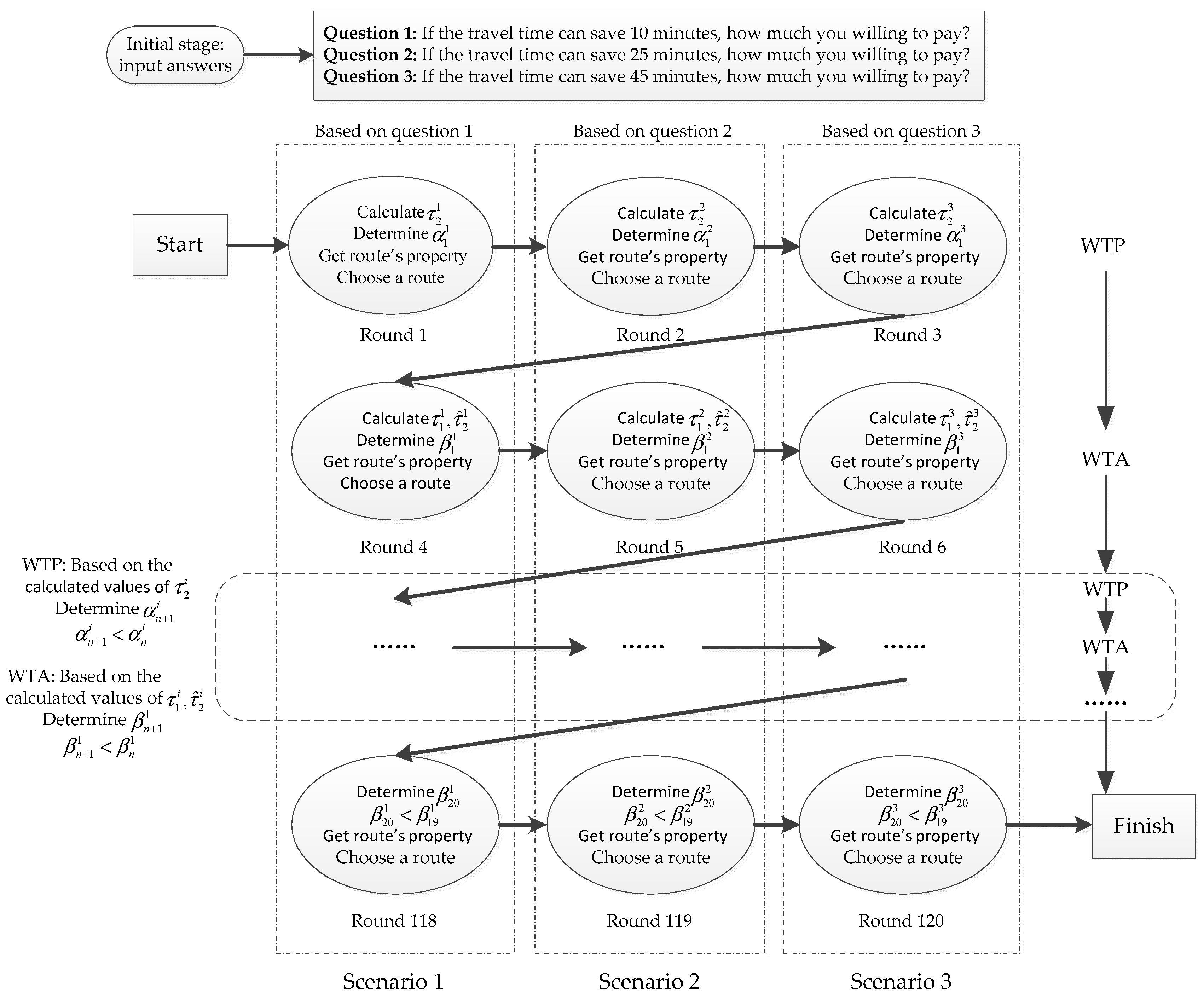
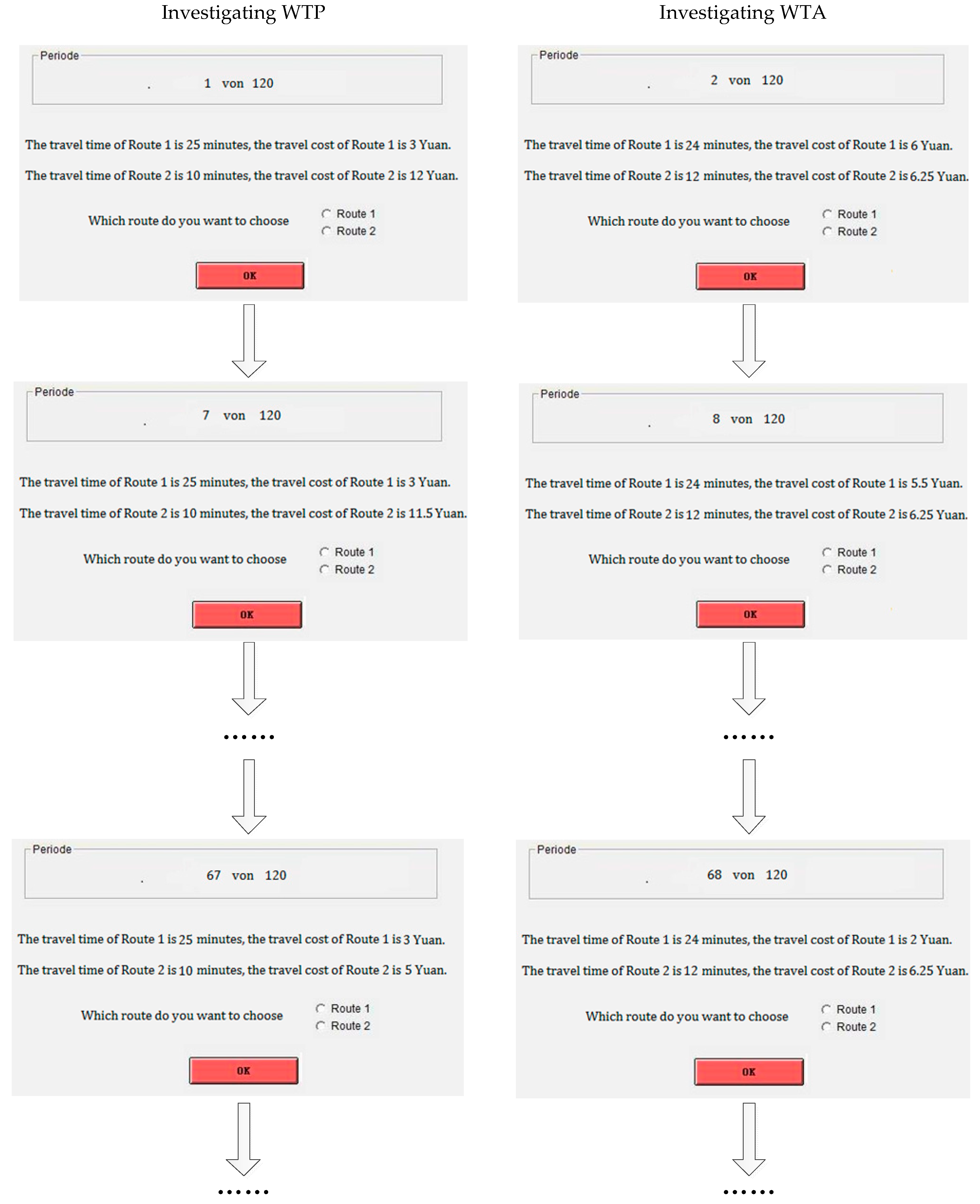
4] research, thus they cannot clearly show that when travelers’ WTP is smaller than their WTA, or when travelers’ WTP is greater than their WTA, how travelers will make their route choices. In addition, how will the scaling effect of travel cost affect travelers’ asymmetric preference? This paper is an extended work of Xu et al.’s research aiming to provide more detailed support as an empirical study. A route choice experiment was conducted to investigate the impact of asymmetric preference on travelers’ inertial route choice. In the experiment, three different travel scenarios (short, middle, and long travel) were designed to collect participants’ route choice data. Then, based on the experimental data, the value of participants’ WTP and WTA were calculated and compared. According to the value of WTP and WTA, participants’ route choice behaviors were analyzed. Moreover, the parameters in Xu’s route choice model were also estimated.
The remainder of this paper is organized as follows. Section 2 describes the status quo-dependent route choice model on how to handle travelers’ route choice behaviors that result from asymmetric preference. Section 3 describes the route choice experiment as well as the data collection procedure. Section 4 presents the calculation and analysis results of participants’ WTP and WTA and route choices in the experiment. Section 5 presents the model parameters estimation. Finally, Section 6 concludes the paper.

2. The Status Quo-Dependent Route Choice Model

For the convenience of readers, the symbols used in this section are summarized as follows:
RWthe set of feasible routes for a given origin-destination (OD) pair w
r the index for a route r R w
j the index for a route j R w \ r
t r w the index for the travel time of route r between OD pair w
t j w the index for the travel time of route j between OD pair w
τ r w the index for the monetary cost of route r between OD pair w
τ j w the index for the monetary cost of route j between OD pair w
c r w the index for a pair of travel time and monetary cost of route r between OD pair w and c r w = ( t r w , τ r w )
Considering two arbitrary non-dominated routes r and j , r , j R w , w W , without loss of generality, it is assumed that t r w t j w and τ r w τ j w . For the travelers on route r , the status quo-dependent travel utility by changing to path j is calculated as Equation (1).
U ( c r w , c j w ) = λ 1 η 1 ( t j w t r w ) + η 2 ( τ r w τ j w )
where U ( c r w , c j w ) is the status quo-dependent travel utility for the travelers on route r , with c r w representing the status quo and c j w the alternative. Parameter λ 1 is the travelers’ loss aversion coefficient of the time cost. η 1 and η 2 are the coefficients that unify time and monetary factors with travel utility. Thus, travelers on route r would suffer a smaller travel time, but they would obtain a larger cost in the aspect of monetary factors, and travelers would stick to route r if and only if the inequality U ( c r w , c j w ) 0 holds. Otherwise, the travelers on route r will change to route j . In addition, U ( c r w , c j w ) 0 holds if and only if
λ 1 η 1 ( t j w t r w ) + η 2 ( τ r w τ j w ) 0 τ r w τ j w λ 1 η 1 η 2 ( t j w t r w ) .
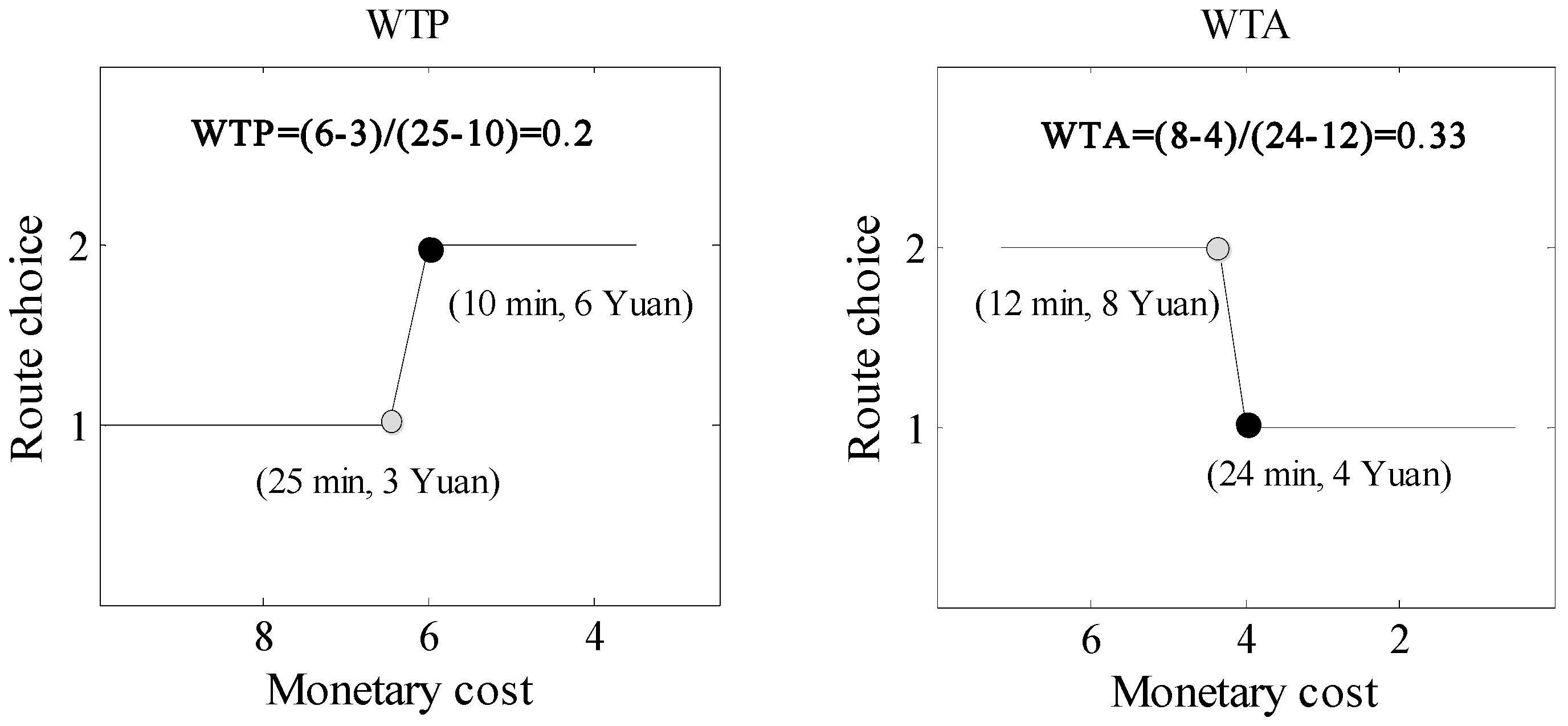
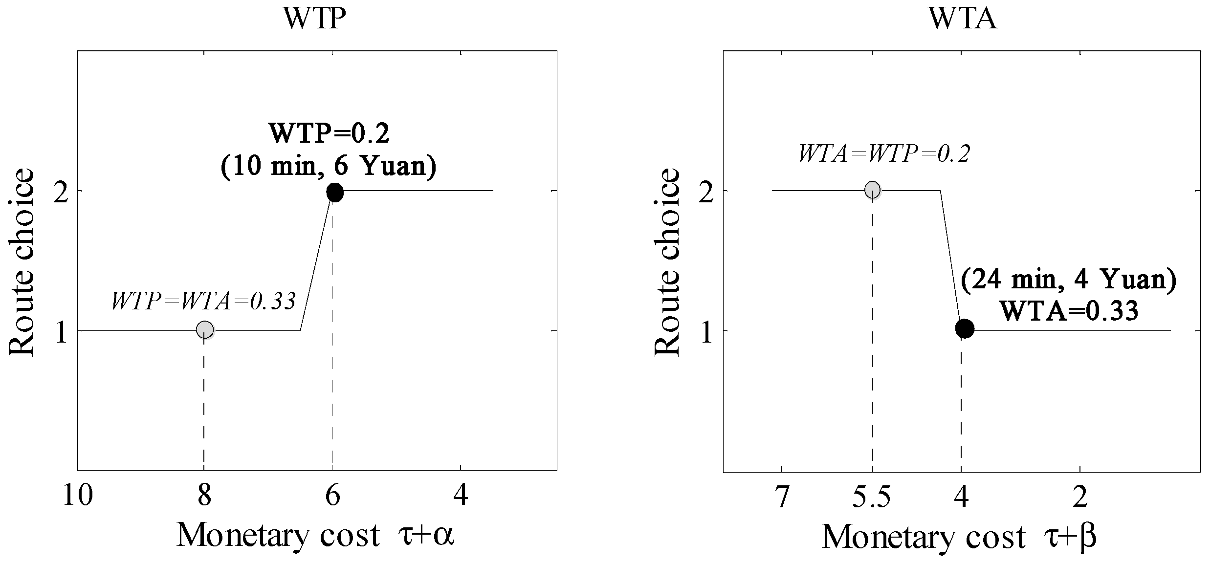
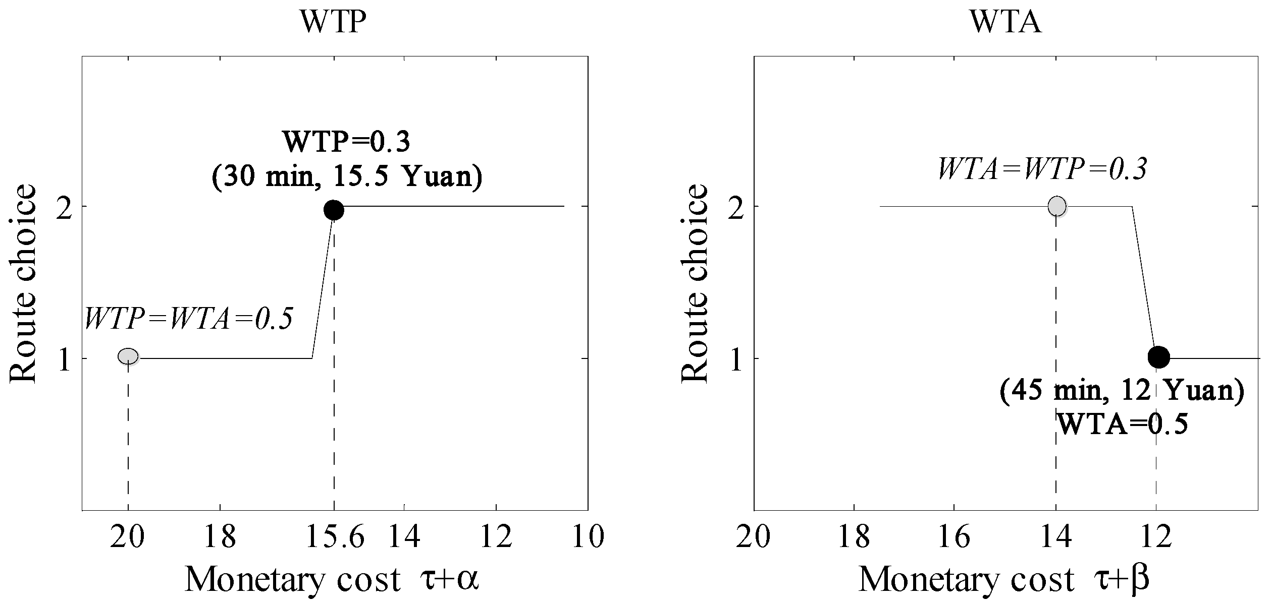
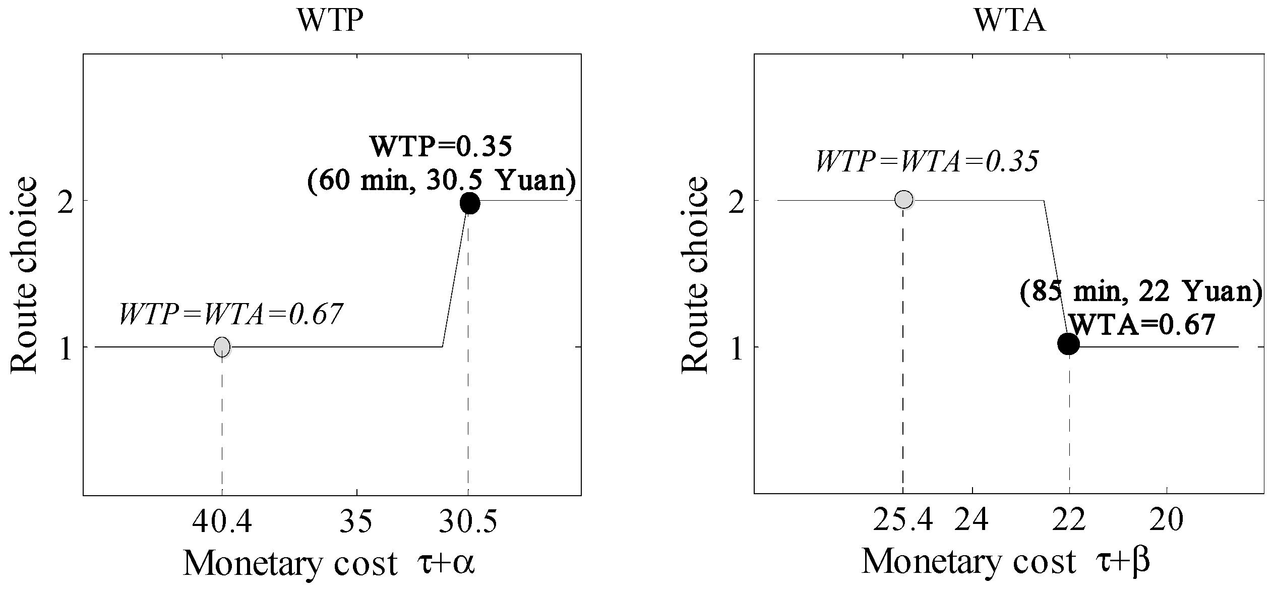
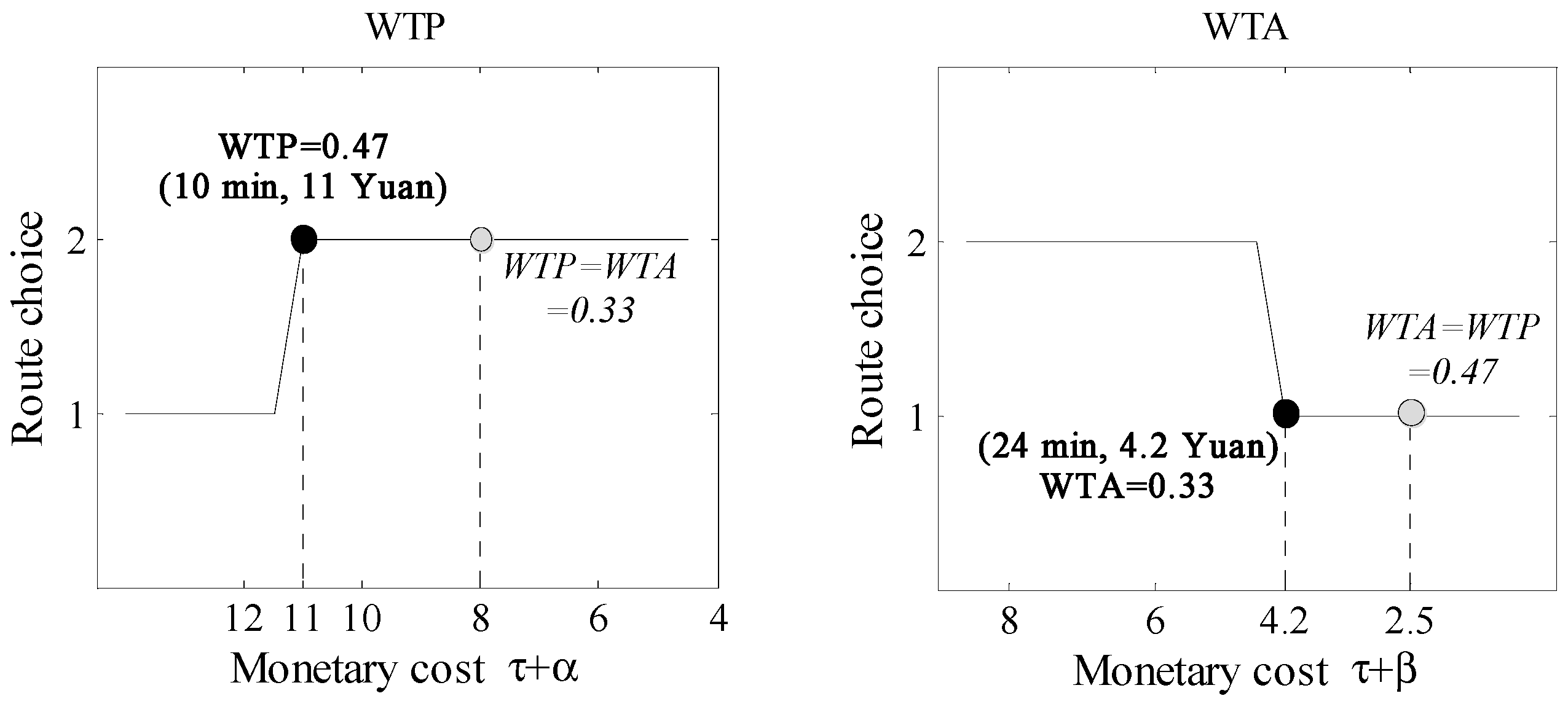
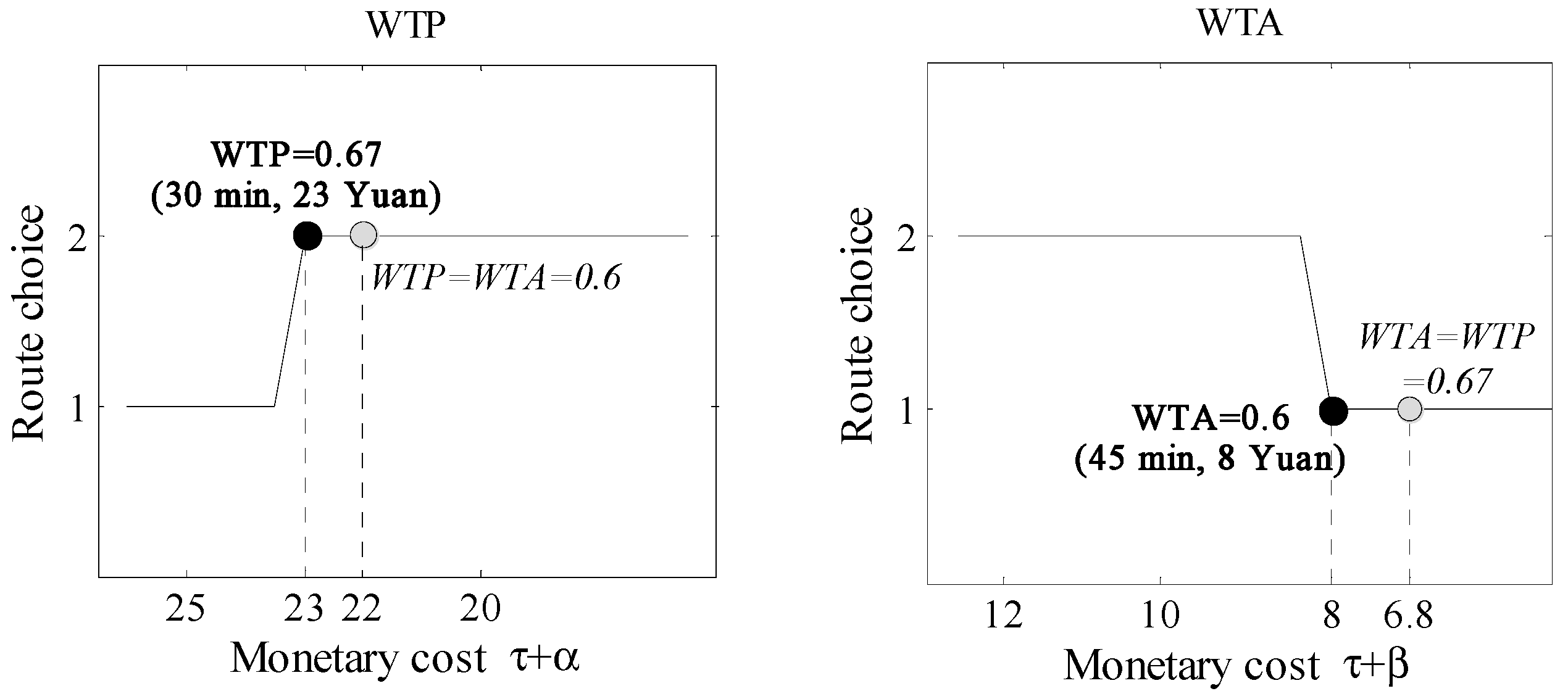
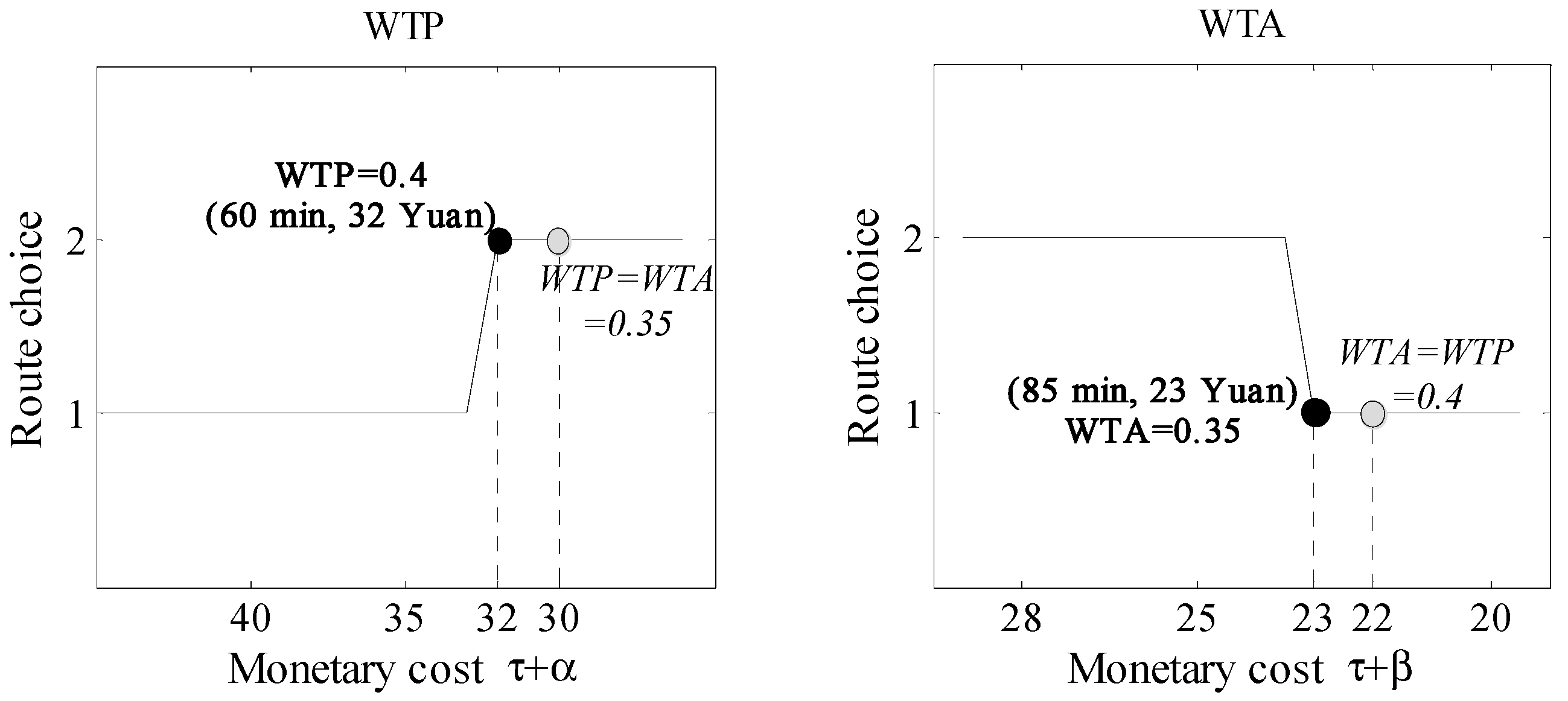
As indicated by Equations (1) and (2), travelers on route r would not change to route j if the potential improvement of monetary cost is not great enough (i.e., less than or equal to the right-hand-side value), and the coefficient λ 1 η 1 / η 2 in Equation (2) is equal to the travelers’ willingness to accept (WTA).
On the other hand, for the travelers on route j the status quo-dependent travel utility by changing to route r , is calculated as Equation (3).
U ( c j w , c r w ) = η 1 ( t j w t r w ) λ 2 η 2 ( τ r w τ j w )
where U ( c j w , c r w ) is the status quo-dependent travel utility for the travelers on route j , with c j w representing the status quo and c r w the alternative. Parameter λ 2 is the travelers’ loss aversion coefficient of the monetary cost. Travelers on route j would suffer a smaller monetary cost, but they would get a larger cost in the aspect of travel time and travelers would stick to route j if and only if the inequality U ( c j w , c r w ) 0 holds. Otherwise, travelers on route j will change to route r . In addition, U ( c j w , c r w ) 0 holds if and only if
η 1 ( t j w t r w ) λ 2 η 2 ( τ r w τ j w ) 0 τ r w τ j w η 1 λ 2 η 2 ( t j w t r w ) .
As indicated by Equations (3) and (4), travelers on route j would not change to route r if the increase in monetary cost is greater than or equal to the right-hand-side value, and the coefficient η 1 / λ 2 η 2 in Equation (4) is equal to the travelers’ willingness to pay (WTP). Then, based on the above analysis, a route choice experiment will be conducted in the following section to verify travelers’ inertial route choices that resulted from asymmetric preference.

3. Experiment Design

The experiment was carried out in the laboratory of the School of Engineering and Management, Nanjing University, in November 2016. We used the z-Tree as our experimental platform [39] to deal with the inputs of all participants’ route choices. Next, we will introduce in detail the participants, experimental design, and procedure in the experiment.

3.1. Participants

In total, 30 participants—12 females and 18 males—were recruited from Nanjing University, and all of them had never participated in a similar experiment. Participants were required to make route choice decisions for a total of 120 test rounds, according to the experimental settings and procedures. During the experiment, participants were not allowed to have any interaction with others.

3.2. Experimental Design

The experimental design included three travel scenarios reflecting three different levels of travel time—short, middle, and long. In each of the scenarios, there were two non-dominated routes, e.g., Route 1 and Route 2, and the route’s status quo is characterized by ( t r , τ r ) . During the experiment, participants needed to choose one’s routes as their travel route, and in each scenario, participants would make route choices for 40 test rounds. Since we focused on travelers’ route choice behaviors in this study, thus, the interaction between travelers and the collective effect of travelers’ behavior on congestion are not considered in the experiment design. Table 1 and Table 2 show the design of travel time and travel cost of two routes in the experiment.
Table 1 is used to investigate participants’ WTP, and Table 2 is used to investigate participants’ WTA. τ 1 i , τ 2 i , and τ ^ 2 i ( i = 1 , 2 , 3 ) represent travel money costs in the three different travel scenarios, and to note that the values of τ 1 i , τ 2 i , and τ ^ 2 i are calculated based on the participants inputting answers about their WTP at the initial stage of the experiment. Figure 1 shows the experimental design steps. As shown in Figure 1, for a participant, at the initial stage of the experiment they needed to input their answers for “if the travel time can save 10 min, how much you willing to pay”, “if the travel time can save 25 min, how much you willing to pay”, and “if the travel time can save 45 min, how much you willing to pay”. Then, based on the three inputted answers, we can calculate the values of τ 1 i , τ 2 i , and τ ^ 2 i ( i = 1 , 2 , 3 ) in Table 1 and Table 2. Additionally, from participants’ own points of view, we can get the ( 25 , 3 ) is equal to ( 10 , τ 2 1 ) , ( 24 , τ 1 1 ) , and ( 12 , τ ^ 2 1 ) (similarly, we can also get the ( 50 , 10 ) is equal to ( 30 , τ 2 2 ) , ( 45 , τ 1 2 ) , and ( 25 , τ ^ 2 2 ) ; ( 90 , 20 ) is equal to ( 60 , τ 2 3 ) , c 1 = ( 85 , τ 1 3 ) , and ( 65 , τ ^ 2 3 ) ). Note that in Table 1 and Table 2 the parameters α n i and β k i ( i = 1 , 2 , 3 ) are constants, which are appended to the monetary cost, and the n and k index for the round of experiment. Moreover, as the experiment progressed, there were α 1 i > α 2 i > > α t i = 0 > > α T i and β 1 i > β 2 i > > β t i = 0 > > β T i . This design ensures that participants will choose Route 1 in the inertial test rounds when investigating their WTP, and they will choose Route 2 in the inertial test rounds when investigating their WTA.

3.3. Procedure

Participants were invited to participate in the experiment at the University laboratory, and each participant was seated separately in front of a computer screen displaying the simulation. In order to encourage realistic behavior, participants were asked to imagine that they were commuters and driving to the workplace. The monthly salary was three times of their school living expenses. They were also informed that from the home to the workplace there were two routes that could be chosen. One route’s travel time was larger than another route’s travel time, but the travel money cost was smaller. For example, Route 1 was a congested road but toll-free, thus the monetary travel cost on Route 1 only consisted of an emission fee, and vehicle operating cost; Route 2 was a toll road but not congested, thus the monetary travel cost on Route 2 consisted of a congestion toll, emission fee, and vehicle operating cost. Note that in the cases of WTA, although a constant β k i was appended to the Route 1′s monetary cost, Route 1 was still cheaper than Route 2 in the experiment. Figure 2 gives examples of actual choice situations in the experiment. No other information was provided before beginning the experiment.
The task included making a series of 120 consecutive route choices. Each test round represented a working day and participants were asked to make daily route choices while driving from home to workplace. Moreover, before the experiment, participants were requested to complete a post-task questionnaire that enquired about their loss aversion of the time cost and the monetary cost. The experimental steps are specified as follows:
(1)
At the initial time, each participant needed to input the answers about their WTP, i.e., how much you are willing to pay if travel time can save 10 min; how much you are willing to pay if travel time can save 25 min; and how much you are willing to pay if travel time can save 45 min.
(2)
During the experiment, in each test round, participants needed to choose one route from two non-dominated routes as their travel route, as can be seen in Figure 2. However, in order to reduce participants’ arbitrary choices as made by the continuous choice under the same scenarios, the three choice scenarios alternated at the computer screen. Moreover, the interval time between each test round was one minute.
(3)
The experiment ended, and each participant received a small gift as a show-up fee.

4. Results and Discussion

4.1. The Values of Participants’ WTP and WTA

Based on the experimental data, the values of participants’ WTP and WTA can be calculated. Note that the WTP refers to the value of a unit time saving in the case of loss in monetary cost, and WTA refers to the monetary compensation a traveler requires to agree to a unit travel time increase. Thus, in the experiment, the participants’ WTP and WTA can be calculated as shown in Figure 3. It is worth mentioning that, for some participants, their initial stated WTP was different from the experimental WTP, in other words, this means that the result of the report is not equal to the result of the action. Considering the action result can better reflect participants’ psychological index of decision-making, therefore, the experimental WTP and WTA were used in this paper. Figure 4 shows the calculation results. It clearly shows that for most participants, their WTP was smaller than WTA in all of three travel scenarios. This means that for these participants, the monetary compensation for the value of unit travel time increasing is larger than the monetary payment for the same value of unit travel time saving. Moreover, the test of null hypothesis shown in Table 3 suggests that the value of WTP is not equal to the value of WTA.
However, regardless of WTP < WTA or WTP > WTA , this result confirms that participants use different measures to distinguish the value of time, rather than constant substitution between money and travel time [33]. Thus, in the experiment, the asymmetric preference exists in participants’ route choices. In addition, for the average values of the WTP, there is WT P 1 < WT P 2 < WT P 3 ( i = 1 ,   2 ,   3 represents Scenario 1, Scenario 2, and Scenario 3). This result indicates that with the increase of the travel time, participants were willing to pay more to save travel time. Then, in order to explain the impact of asymmetric preference on participants’ inertial route choices, in the following subsection, participants’ route choice behaviors will be analyzed.

4.2. Influence of Asymmetric Preference on Participants’ Route Choices

Since in the experiment, many participants’ WTP < WTA or WTP > WTA , the impact of asymmetric preference on participants’ route choices will be discussed with the two cases, i.e., WTP < WTA and WTP > WTA .
Case 1: WTP < WTA
In this subsection, Participant 2 will be taken as an example, and Figure 5, Figure 6 and Figure 7 show Participant 2′s route choices in the experiment under three different travel scenarios. As shown in Figure 5, in Scenario 1, Participant 2′s WTP equals 0.2 and WTA equals 0.33. Then, assuming that if Participant 2′s WTP equals WTA (i.e., WTP = WTA = 0.33 ), they should switch to Route 2 when its travel monetary cost is 8. However, in fact, Participant 2 continues to choose Route 1 until Route 2′s travel monetary cost is 6. On the other hand, assuming that if Participant 2′s WTA equals WTP (i.e., WTP = WTA = 0.2 ), they should switch to Route 1 when its travel monetary cost is 5.5. However, in fact, Participant 2 continues to choose Route 2 until Route 1′s travel monetary cost is 4. Moreover, for Participant 2 (even those other participants whose WTP was smaller than WTA), similar phenomena can be found in the other two scenarios. Therefore, when the participants’ WTP was smaller than WTA, the asymmetric preference can make them stick to the current routes until one alternative route’s monetary cost is enough to tempt them to choose. This analysis result verifies that asymmetric preference (i.e., WTP < WTA ) can lead travelers to make inertial choices (e.g., stick to the current route).
Case 2: WTP > WTA
In this subsection, Participant 10 (Scenario 1), Participant 22 (Scenario 2), and Participant 21 (Scenario 3) will be taken as examples, and Figure 8, Figure 9 and Figure 10 show participants’ route choices in the experiment under three different travel scenarios. As shown in Figure 8, in Scenario 1, Participant 10’s WTP equals 0.47 and WTA equals 0.33. Then, assuming that if Participant 10’s WTP equals WTA (i.e., WTP = WTA = 0.33 ), they should switch to Route 2 when its travel monetary cost is 8. However, in fact, Participant 10 switches to Route 2 when its travel monetary cost is 11. On the other hand, assuming that if Participant 10’s WTA equals WTP (i.e., WTA = WTP = 0.47 ), they should switch to Route 1 when its travel monetary cost is 2.5. However, in fact Participant 10 switches to Route 1 when its travel monetary cost is 4.2. Moreover, for another two participants, similar phenomena can be found in the other two scenarios. Therefore, when participants’ WTP was larger than WTA, the asymmetric preference can make them tend to choose a route with the shortest travel time.
The above analysis results suggest that when participants’ WTP is smaller than WTA, the asymmetric preference can make them stick to the current routes. Next, based on the observation data, the parameters λ 1 , λ 2 , η 1 , and η 2 in Xu’s [4] status quo-dependent route choice model will be estimated.

5. Model Parameters Estimation

5.1. Estimation of λ 1 and λ 2

The cumulative prospect theory (CPT), which was proposed by Tversky and Kahneman [40], is a valid utility measurement system. Many researchers used CPT to study individual’s risk attitude and choice behavior under uncertainty over the past years. Xu et al. [41] developed a general travel decision-making rule utilizing CPT to investigate travelers’ risk attitudes and route choice behaviors under uncertainty. Zhang et al. [42], based on the CPT, developed a day-to-day route-choice learning model with friends’ travel information. Therefore, in this subsection, the cumulative prospect theory (CPT) was applied to measure participants’ risk attitudes, i.e., loss aversion of travel time and travel monetary cost. Without loss of generality, let x 0 define a reference point in the outcome domain, and the value function can be defined as Equation (5), and the weighting function can be defined as Equation (6).
v ( x ) = { ( x x 0 ) α , x > x 0 λ ( x 0 x ) β , x x 0
w ( p i ) = p i γ / [ p i γ + ( 1 p i ) γ ] 1 / γ
where the parameters α 1 , β 1 measure the degree of the diminishing sensitivity to change in both directions from the reference point x 0 , parameter λ 1 captures the degree of loss aversion, parameters 0 < γ < 1 reflect the level of distortion in the probability judgment. p i is the probability of an outcome x i . Figure 11 illustrates the value function and the weighting function. Suppose an alternative denoted by the pair ( x ; p ) is composed of m + n + 1 possible outcomes x m < < x 0 < < x n with probabilities p m , , p n , respectively. Then, the cumulative decision weights are defined as follows:
π i + ( p i ) = w + ( p i + + p n ) w + ( p i + 1 + + p n ) , 0 i n 1
π j ( p j ) = w ( p m + + p j ) w ( p m + + p j 1 ) , 1 m j 0 .
Accordingly, the CPT value of ( x ; p ) can be calculated by Equation (9).
U ( x ; p ) = i = 0 n 1 v ( x ) π i + ( p i ) + j = 1 m 0 v ( x ) π j ( p j )
Firstly, participants were requested to complete a post-task questionnaire. Then, based on the survey data from the questionnaire, the parameter λ 1 and λ 2 were estimated. The design of the questionnaire considered the following two scenes:
Scene 1
(Investigate the loss aversion of the travel time): The travel times on both routes (Route A and Route B) are likely to increase because of congestion. Let ( t 1 , p 1 % ; t 2 , p 2 % ) denote the distribution of travel time on each route. For a traveler, there is a probability of p 1 % to accomplish the trip with t 1 more minutes, a probability of p 2 % to accomplish the trip with t 2 more minutes, and a probability of 1 p 1 % p 2 % with no extra time.
Scene 2
(Investigate the loss aversion of the travel monetary cost): The travel costs on both routes (Route R and Route S) are likely to increase because of the late penalty. Let ( c 1 , p 1 % ; c 2 , p 2 % ) denote the distribution of travel cost on each route. For a traveler, there is a probability of p 1 % to accomplish the trip with c 1 more costs (Yuan, Chinese currency), a probability of p 2 % to accomplish the trip with c 2 more costs, and a probability of 1 p 1 % p 2 % with no extra costs.
The route choice preferences of participants between A and B are shown in Table 4. The route choice preferences of participants between R and S are shown in Table 5.
Then, based on the survey data in Table 4 and Table 5, the values of parameters λ 1 and λ 2 can be estimated using the least squares method and the cumulative squared residual can be given by following Equations (10) and (11), respectively:
f ( β 1 , λ 1 , δ ) = k = 1 k = 5 ( A k % P ( A k > B k ) ) 2
f ( β 2 , λ 2 , δ ) = k = 6 k = 12 ( R k % P ( R k > S k ) ) 2
where A % is the proportion of choosing Route A in case k , P ( A k > B k ) is the probability that Route A is more valuable than Route B in case of k , and P ( A k > B k ) can be given by Equation (12). R % is the proportion of choosing Route R in case of k , P ( R k > S k ) is the probability that Route R is more valuable than Route S in case k , and P ( R k > S k ) can be given by Equation (12). Here, U ( ) is the route’s cumulative prospect value and it can be calculated by Equation (9).
P ( A k > B k ) = 1 1 + exp ( U ( B k ) U ( A k ) )
P ( R k > S k ) = 1 1 + exp ( U ( S k ) U ( R k ) )
Note that in this paper, the value of parameter δ is set as 0.74, which was estimated by Wu and Gonzalez [43]. Participants’ perception errors of the cumulative prospect value are assumed to follow the independent and identical Gumbel distributions. Then, based on these settings, the estimation values of β 1 is 0.35 and λ 1 is 1.41 in Scene 1; β 2 is 0.23 and λ 2 is 1.26 in Scene 2.

5.2. Estimation of η 1 and η 2

Until now, we have estimated the values of parameters λ 1 and λ 2 , associated with the CPT-based utility measurement system. Specifically, λ 1 = 1.41 and λ 2 = 1.26 . With them, based on the experimental data, we used the least squares method to estimate the values of parameters η 1 and η 2 . Data of three thousand and six hundred observations of 30 participants were used. Table 6 presents the estimation results.
As shown in Table 6, the estimation values of all parameters are positive and significant. Based on the estimation values of λ 1 , λ 2 , η 1 , and η 2 , participants’ WTP (i.e., η 1 / λ 2 η 2 ) and WTA (i.e., λ 1 η 1 / η 2 ) can be calculated. Table 5 also shows the results of the calculation. As shown in Table 6, there is W T P 1 < W T P 2 < W T P 3 and W T A 1 < W T A 2 < W T A 3 ( i = 1 , 2 , 3 represents Scenario 1, Scenario 2, and Scenario 3). These results are consistent with the aforementioned data analysis. Moreover, the calculation results of W T P < W T A for three scenarios further explain that the asymmetric preference exists in participants’ route choices.

6. Conclusions

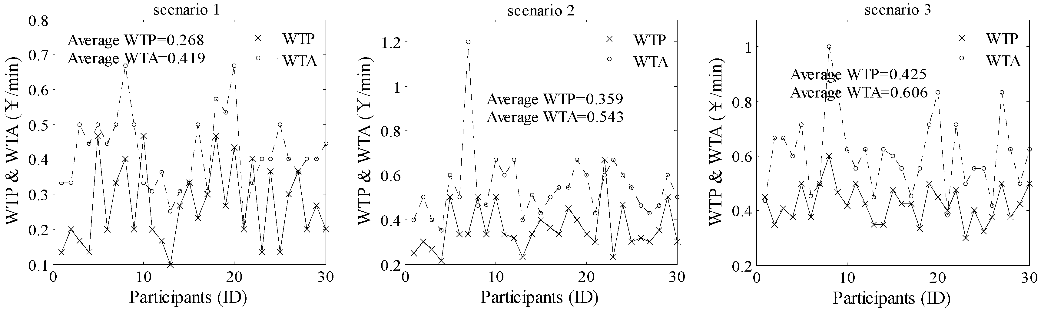
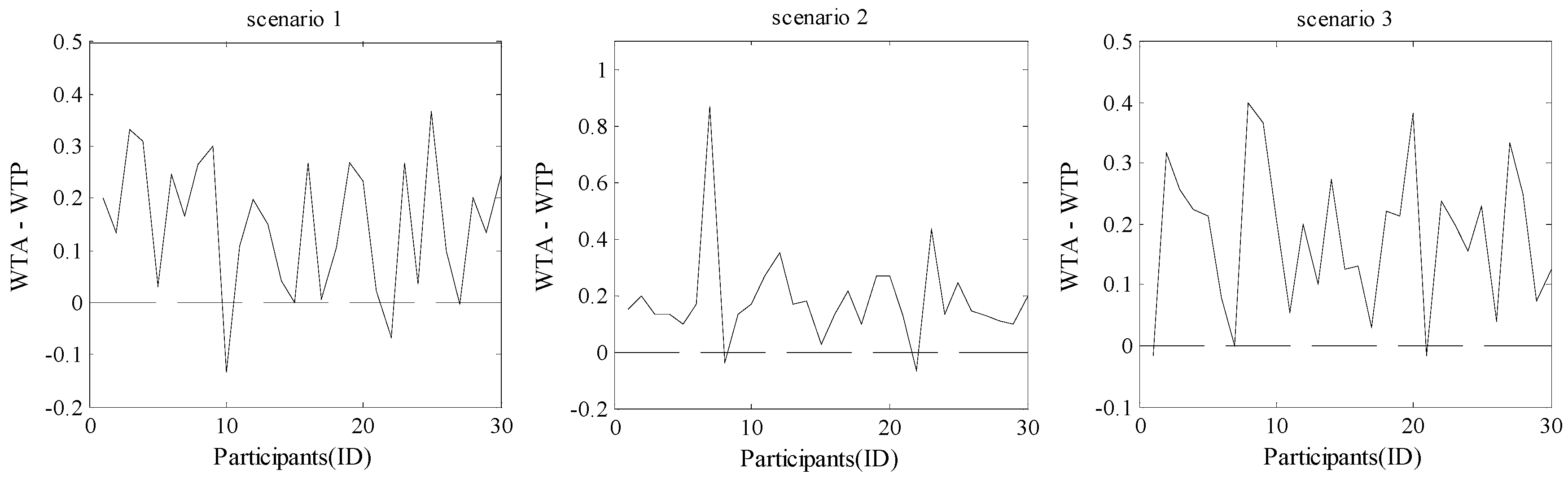
In this research, a route choice experiment was conducted to investigate travelers’ inertial route choice behaviors that resulted from asymmetric preference. Through data analysis, we can confirm that in the experiment participants used different measures to distinguish the value of time rather than constant substitution between money and travel time. Additionally, asymmetric preference significantly exists in participants’ route choices. Especially, for most participants, their WTP was smaller than WTA, and this makes them stick to the current route until one alternative route’s monetary cost is enough to tempt them to choose.
The value of this study lies in verifying travelers’ inertial route choices that resulted from asymmetric preference and estimating the values of parameters in Xu’s [4] status quo-dependent route choice model. Moreover, by considering the asymmetric preference, we can explain why some travelers stick to a toll lane, even when there is an alternative road that is slightly better. However, there are some limitations in our experimental design. Firstly, we used the questionnaire survey data of 30 participants to estimate the values of parameters λ 1 and λ 2 . However, a behavioral experiment is needed to collect individuals’ route-choice data to estimate the values of parameters λ 1 and λ 2 . Secondly, as noted earlier, our experimental design was conducted with a lack of interaction between the participants’ choices. Thus, there is meaningful reason for designing a behavioral experiment, and to incorporate the asymmetric preference into traffic equilibrium modeling.

Author Contributions

Model construction, experiment design, software, analysis of results and model parameters estimation: K.L.; introduction writing, model parameters estimation: Y.X.

Funding

This work was supported by a national natural science foundation of China [No. 71571097] and a humanities and social sciences project of Anhui, China [No. SK2018A0025].

Conflicts of Interest

The authors declare no conflict of interest.

References

  1. Wardrop, J.G. Some theoretical aspects of road traffic research. Proc. Inst. Civ. Eng. 1952, 1, 325–378. [Google Scholar] [CrossRef]
  2. Avineri, E. The effect of reference point on stochastic network equilibrium. Transp. Sci. 2006, 40, 409–420. [Google Scholar] [CrossRef]
  3. Chen, R.B.; Mahmassani, H.S. Learning and risk attitudes in route choice dynamics. In Expanding Sphere of Travel Behavior Research, Proceedings of the 11th International Conference, Orlando, FL, USA, 30 September–3 October 2009; Kitamura, R., Yoshii, T., Eds.; Emerald: Bingley, UK, 2009; pp. 791–818. [Google Scholar]
  4. Xu, H.L.; Yang, H.; Zhou, J.; Yin, Y.F. A route choice model with context-dependent value of time. Transp. Sci. 2017, 51, 536–548. [Google Scholar] [CrossRef]
  5. Nakayama, S.; Kitamura, R.; Fujii, S. Drivers’ route choice rules and network behavior: Do drivers become rational and homogeneous through learning? Transp. Res. Rec. 2001, 1752, 62–68. [Google Scholar] [CrossRef]
  6. Avineri, E.; Prashker, J.N. Violations of expected utility theory in route-choice stated preferences: Certainty effect and inflation of small probabilities. Transp. Res. Rec. 2004, 1894, 222–229. [Google Scholar] [CrossRef]
  7. Zhu, S. The roads taken: Theory and Evidence on Route Choice in the Wake of the I-35w Mississippi River Bridge Collapse and Reconstruction. Ph.D. Thesis, University of Minnesota, Mineapolis, MN, USA, 2010. [Google Scholar]
  8. Simon, H.A. A Behavioral Model of Rational Choice. Q. J. Econ. 1955, 69, 99–118. [Google Scholar] [CrossRef]
  9. Mahmassani, H.S.; Chang, G. On boundedly rational user equilibrium in transportation systems. Transp. Sci. 1987, 21, 89–99. [Google Scholar] [CrossRef]
  10. Lou, Y.; Yin, Y.; Lawphongpanich, S. Robust congestion pricing under boundedly rational user equilibrium. Transp. Res. Part B Methodol. 2010, 44, 15–28. [Google Scholar] [CrossRef]
  11. Zhao, C.L.; Huang, H.J. Experiment of boundedly rational route choice behavior and the model under satisficing rule. Transp. Res. Part C Emerg. Technol. 2016, 68, 22–37. [Google Scholar] [CrossRef]
  12. Alós-Ferrer, C.; Hügelschäfer, S.; Li, J. Inertia and Decision Making. Front. Psychol. 2016, 7, 1–9. [Google Scholar] [CrossRef]
  13. Huff, J.O.; Huff, A.S.; Thomas, H. Strategic renewal and the interaction of cumulative stress and inertia. Strateg. Manag. J. 1992, 13, 55–75. [Google Scholar] [CrossRef]
  14. Sautua, S.I. Does Uncertainty Cause Inertia in Decision Making? An EXPERIMENTAL Study of the Role of Regret Aversion and Indecisiveness. Working Paper. 2016. Available online: https://www.researchgate.net/publication/301650273 (accessed on 8 January 2019).
  15. Chorus, C.G.; Dellaert, B.G.C. Travel Choice Inertia: The Joint Role of Risk Aversion and Learning. J. Transp. Econ. Policy 2012, 46, 139–155. [Google Scholar]
  16. Becker, G.S. The Economic Approach to Human Behavior; University of Chicago Press: Chicago, IL, USA, 1976. [Google Scholar]
  17. Gal, D. A psychological law of inertia and the illusion of loss aversion. Judgm. Decis. Mak. 2006, 1, 23–32. [Google Scholar]
  18. Kahneman, D.; Knetsch, J.L.; Thaler, R.H. The endowment effect, loss aversion, and status quo bias. J. Econ. Perspect. 1991, 5, 193–206. [Google Scholar] [CrossRef]
  19. Miravete, E.J.; Palacios-Huerta, I. Consumer inertia, choice dependence, and learning from experience in a repeated decision problem. Rev. Econ. Stat. 2014, 96, 524–537. [Google Scholar] [CrossRef]
  20. Chorus, C.G. Risk aversion, regret aversion and travel choice inertia: An experimental study. Transp. Plan. Technol. 2014, 37, 321–332. [Google Scholar] [CrossRef]
  21. Van Exel, N.J.A. Behavioural Economic Perspectives on Inertia in Travel Decision Making. Ph.D. Thesis, Vrije Universiteit Amsterdam, Amsterdam, The Netherlands, 2011. [Google Scholar]
  22. Lindsey, R. State-dependent congestion pricing with reference dependent preferences. Transp. Res. Part B Methodol. 2011, 45, 1501–1526. [Google Scholar] [CrossRef]
  23. Train, K.E. Discrete Choice Methods with Simulation; The Cambridge University Press: Cambridge, UK, 2003. [Google Scholar]
  24. Xie, C.; Liu, Z.G. On the stochastic network equilibrium with heterogeneous choice inertia. Transp. Res. Part B Methodol. 2014, 66, 90–109. [Google Scholar] [CrossRef]
  25. Guo, X.; Liu, H.X. Bounded rationality and irreversible network change. Transp. Res. Part B Methodol. 2011, 45, 1606–1618. [Google Scholar] [CrossRef] [Green Version]
  26. Vreeswijk, J.D.; Landman, R.L.; Van Berkum, E.C.; Hegyi, A. Improving the road network performance with dynamic route guidance by considering the indifference band of road users. Intell. Transp. Syst. 2015, 9, 897–906. [Google Scholar] [CrossRef] [Green Version]
  27. Site, P.D.; Filippi, F. Stochastic user equilibrium and value-of-time analysis with reference-dependent route choice. Eur. J. Transp. Infrastruct. Res. 2011, 2, 194–218. [Google Scholar]
  28. Zhang, J.L.; Yang, H. Modeling route choice inertia in network equilibrium with heterogeneous prevailing choice sets. Transport. Res. Part. C Emerg. Technol. 2015, 57, 42–54. [Google Scholar] [CrossRef]
  29. Gärling, T.; Axhausen, K.W. Introduction: Habitual travel choice. Transportation 2003, 30, 1–11. [Google Scholar] [CrossRef]
  30. Kim, H.; Oh, J.S.; Jayakrishnan, R. Effects of user equilibrium assumptions on network traffic pattern. Ksce J. Civ. Eng. 2009, 13, 117–127. [Google Scholar] [CrossRef]
  31. Denrell, J.; March, J.G. Adaptation as information restriction: The hot stove effect. Organ. Sci. 2001, 12, 523–538. [Google Scholar] [CrossRef]
  32. Thaler, R. Toward a positive theory of consumer choice. J. Econ. Behav. Organ. 1980, 1, 39–60. [Google Scholar] [CrossRef]
  33. Small, K.A. Valuation of travel time. Econ. Transp. 2012, 1, 2–14. [Google Scholar] [CrossRef]
  34. Boyce, R.R.; Brown, T.C.; McCledlland, G.H. An experimental examination of intrinsic values as a source of the WTS-WTP disparity. Am. Econ. Rev. 1992, 82, 1366–1373. [Google Scholar]
  35. De Borger, B.; Fosgerau, M. The trade-off between money and travel time: A test of the theory of reference-dependent preferences. J. Urban Econ. 2008, 64, 101–115. [Google Scholar] [CrossRef] [Green Version]
  36. Hess, S.; Rose, J.M.; Hensher, D.A. Asymmetric preference formation in willingness to pay estimates in discrete choice models. Transp. Res. Part. E Logist. Transp. Rev. 2008, 44, 847–863. [Google Scholar] [CrossRef] [Green Version]
  37. Schmidt, U.; Traub, S. An experimental investigation of the disparity between WTA and WTP for lotteries. Theory Decis. 2009, 66, 229–262. [Google Scholar] [CrossRef]
  38. Masiero, L.; Hensher, D.A. Shift of reference point and implications on behavioral reaction to gains and losses. Transportation 2011, 38, 249–271. [Google Scholar] [CrossRef]
  39. Urs Fischbacher. z-Tree: Zurich toolbox for ready-made economic experiments. Exp. Econ. 2007, 10, 171–178. [Google Scholar] [CrossRef] [Green Version]
  40. Tversky, A.; Kahneman, D. Advances in prospect theory: Cumulative representation of uncertainty. J. Risk Uncertain. 1992, 5, 297–323. [Google Scholar] [CrossRef] [Green Version]
  41. Xu, H.L.; Zhou, J.; Xu, W. A decision-making rule for modeling travelers’ route choice behavior based on cumulative prospect theory. Transp. Res. Part. C Emerg. Technol. 2011, 19, 218–228. [Google Scholar] [CrossRef]
  42. Zhang, C.; Liu, T.L.; Huang, H.J.; Chen, J. A cumulative prospect theory approach to commuters’ day-to-day route-choice modeling with friends’ travel information. Transp. Res. Part C Emerg. Technol. 2018, 86, 527–548. [Google Scholar] [CrossRef]
  43. Wu, G.; Gonzalez, R. Curvature of the probability weighting function. Manag. Sci. 1996, 12, 1676–1690. [Google Scholar] [CrossRef]
Figure 1. The design of experiment. WTP: willingness to pay; WTA: willingness to accept.
Symmetry 11 00066 g001
Figure 2. Snapshot of the route choice simulation window (Scenario 1).
Symmetry 11 00066 g002
Figure 3. The calculation method of WTP and WTA.
Symmetry 11 00066 g003
Figure 4. The value of WTP and WTA for all participants in three travel scenarios.
Symmetry 11 00066 g004aSymmetry 11 00066 g004b
Figure 5. Scenario 1—short travel time.
Symmetry 11 00066 g005
Figure 6. Scenario 2—middle travel time.
Symmetry 11 00066 g006
Figure 7. Scenario 3—long travel time.
Symmetry 11 00066 g007
Figure 8. Scenario 1—short travel time (Participant 10).
Symmetry 11 00066 g008
Figure 9. Scenario 2—middle travel time (Participant 22).
Symmetry 11 00066 g009
Figure 10. Scenario 3—long travel time (Participant 21).
Symmetry 11 00066 g010
Figure 11. Value function and weighting function.
Symmetry 11 00066 g011
Table 1. Investigating participants’ willingness to pay (travel time *, monetary cost **).
Scenario 1 (Short)Scenario 2 (Middle)Scenario 3 (Long)
Route 1Route 2Route 1Route 2Route 1Route 2
(25 *, 3 **)(10, τ 2 1 + α n 1 )(50, 10)(30, τ 2 2 + α n 2 )(90, 20)(60, τ 2 3 + α n 3 )
* The unit of travel time is minute. ** The unit of monetary cost is Yuan, which is the Chinese currency unit.
Table 2. Investigating participants’ willingness to accept (travel time, monetary cost).
Scenario 1 (Short)Scenario 2 (Middle)Scenario 3 (Long)
Route 1Route 2Route 1Route 2Route 1Route 2
(24, τ 1 1 + β k 1 )(12, τ ^ 2 1 )(45, τ 1 2 + β k 2 )(25, τ ^ 2 2 )(85, τ 1 3 + β k 3 )(65, τ ^ 2 3 )
Table 3. Hypothesis test.
Null Hypothesist-TestStd. err95% Confidence IntervalSig.
LowerUpper
H0: WTP = WTA5.1710.2140.4860.1080.013
Table 4. Results of route choice in Scene 1.
CaseRoute A Route B
SettingsNumber/Proportion SettingsNumber/Proportion
1(20, 10%)1653.3% (10, 20%)1446.7%
2(20, 10%; 10, 80%)2066.7% (10, 100%)1033.3%
3(20, 10%; 10, 20%)1756.7% (10, 40%)1343.3%
4(20, 10%; 10, 70%)1446.7% (10, 90%)1653.3%
5(20, 10%; 10, 30%)1860.0% (10, 50%)1240.0%
Table 5. Results of route choice in Scene 2.
CaseRoute R Route S
SettingsNumber/Proportion SettingsNumber/Proportion
6(10, 10%)1756.7% (5, 20%)1343.3%
7(10, 10%; 5, 80%)2273.3% (5, 100%)826.7%
8(10, 10%; 5, 20%)1653.3% (5, 40%)1446.7%
9(10, 10%; 5, 70%)1343.3% (5, 90%)1756.7%
10(10, 10%; 5, 30%)1963.3% (5, 50%)1136.7%
Table 6. Model estimation results.
Scenario 1 (Short)Scenario 2 (Middle)Scenario 3 (Long)
η 1 1 η 2 1 η 1 2 η 2 2 η 1 3 η 2 3
Estimate0.4621.5130.5741.4210.6321.357
Std. error0.2140.4760.2460.4320.2840.407
t-Test2.0404.7412.2684.4702.4414.132
P-Value<0.001<0.001<0.010<0.001<0.001<0.001
W T P = η 1 / λ 2 η 2 0.2420.3210.364
W T A = λ 1 η 1 / η 2 0.4270.5700.647

