Chronic Liver Disease Classification Using Hybrid Whale Optimization with Simulated Annealing and Ensemble Classifier

Abstract

Chronic liver disease (CLD), which indicates the inflammatory condition of the liver, leads to cirrhosis or even partial or total liver dysfunction when left untreated. A non-invasive approach for evaluating CLD with computed tomography (CT) images is proposed using an ensemble of classifiers. To accurately classify CLD, the hybrid whale optimization algorithm with simulated annealing (WOA-SA) is used in selecting an optimal set of features. The proposed method employs seven sets of features with a total of 73–3D (three-dimensional) texture features. A hybrid ensemble classifier with support vector machine (SVM), k—Nearest Neighbor (k-NN), and random forest (RF) classifiers are used to classify liver diseases. Experimental analysis is performed on clinical CT images datasets, which include normal liver, fatty liver, metastasis, cirrhosis, and cancerous samples. The optimal features selected using the WOA-SA improve the accuracy of CLD classification for the five classes of diseases mentioned above. The accuracy of the liver classification using ensemble classifier yields approximately 98% with a 95% confidence interval (CI) of (0.7789, 1.0000) and an error rate of 1.9%. The performance of the proposed method is compared with two existing algorithms and the sensitivity and specificity yield an overall average of 96% and 93%, with 95% confidence interval of (0.7513, 1.0000) and (0.7126, 1.0000), respectively. Classification of CLD based on ensemble classifier illustrates the effectiveness of the proposed method and the comparison analysis demonstrates the superiority of the methodology.

1. Introduction

The human liver is the largest internal organ of the body and liver disease is among the critical diseases that affect the normal, healthy stature of a human due to various reasons [1]. There are various types of liver disease, namely fatty liver, cirrhosis, hepatitis, chronic liver disease, liver cancer and liver tumor, etc. [2]. Excess triglyceride fat accumulation leads to fatty liver [3]. Hepatitis virus infection in the liver is developed due to excessive consumption of alcohol, detrimental food habits, etc. [3]. Hepatitis [4] can result in acute and chronic infection. Cirrhosis [5] is fibrous tissue that replaces the dead liver cells with fibroid. Metastatic tumors are cancerous tumors in the liver that spread from cancer affected in other organs [6,7]. Chronic liver disease (CLD) is estimated worldwide with figures up to 844 million people and has a mortality rate of about two million per year. The World Health Organization (WHO) [8] states that death tolls worldwide rose to 50 million per year over two decades due to cirrhosis and liver cancer. In 2015, deaths caused by liver diseases due to alcohol were reported to be an age-standardized rate of 14.2 deaths per 100,000 population by the global studies made in the United Kingdom [9]. The diagnosis of liver diseases can be analyzed using ultrasonography, magnetic resonance imaging (MRI), computed tomography (CT) [10], etc. However, the advanced level of curing can be obtained only by liver transplantation [11]. The ultrasound-based procedures are constrained by high technical failure rates. They are both machine and operator dependent with low accuracy in morbidly obese persons and do not produce reproducible, continuous ranges of quantitative information [2,12]. The CT and MRI [13] are the two broadly utilized imaging tests for diagnosing various problems in human anatomy, including abdominal infections. MRI provides improved results with soft tissues when the scanning process involves contrast enhanced liver specific agents [14], as it will be visibly annotated for its boundary with abdominal CT images. Moreover, MRI scans are costlier [15] than CT image scans. The CT based methods [16] have high resolution with challenging visualization, efficient data transfer, and are well-suited for solid organs in human anatomy [17], whereas MRI [18] suffers spatial distortion of tissue intensity caused by main magnetic field inhomogenity. The benefits of using ionizing imaging modality are faster scan times, improved spatial resolution, and advanced multi-planar reconstruction techniques. All of these have increased the utilization of CT for every anatomic abnormality over non-ionizing imaging modalities. The ionizing radiation dose received during a CT scan depends on the protocol, such as the radiographic factors and the number of series obtained. Generally, a CT scan of the abdomen exposes the patient to about 20 mSv of IR depending on the protocol, but on average, it increases the risk of fatal cancer by about one in 1000. The quick and precise forecast of liver disease permits early detection and viable medications and is important on the grounds that it spares patients from advanced sicknesses [19]. For this early detection, liver biopsy is the gold standard [20] invasive approach for CLD. However, it has life threatening complications due to transient pain, anxiety, and discomfort [21]. The optical biopsy of liver tissue [22] using optic fiber had been marked with quantitative interpretations of the measurements. Non-invasive methods for CLD diagnosis using computer-aided diagnosis (CAD) yield similar accuracy like liver biopsy and [23,24] have proposed the same. Two crucial steps play vital roles in the non-invasive methods of CLD classification, namely feature extraction and classification. Image-based features using textures is an active research area in CLD classification. Machine learning algorithms (MLA) such as neural networks [25], support vector machine (SVM) [26], ensemble classifier [27], etc., are used for texture-based CLD classification in the current scenario. Many scientific articles that report different approaches for feature extraction and classification exist.

One effective tool to characterize normal and diseased livers is by means of texture analysis, as it describes the local spatial variations in the image. This texture feature is the mathematical parameter computed from the two-dimensional (2D)/three-dimensional (3D) space of the pixels/voxels. Among the various texture feature extraction algorithms, the co-occurrence matrix (CM) based Haralick method [28] is widely used. In medical imaging, statistical texture features proved to have higher recognition. These features have been used in various applications such as fetal lung maturity [29], liver tissue characterization [30], prostate cancer recognition [31], etc. In the proposed method, different texture features are constructed from the identified regions of interest using second and higher order statistical features [32].

Similarly, for efficient CLD classification, researchers preferred MLA such as SVM, random forests (RF), artificial neural network (ANN), etc., [33,34]. However, RF, which is a prominent classifier, may be prompted to vulnerabilities [35]. ANN, on the other hand, classifies liver diseases effectively, but it requires higher computational cost and is prone to overfitting [36]. SVM is robust to noise and leads to efficient classification results [37].

To recognize the fatty liver disease (FLD), Acharya et al. [38] proposed the texture feature based FLD classification and discussed various diagnostic techniques. The authors adopted the cutting edge ultrasound-based CAD techniques that use a scope of image texture based features like entropy, local binary pattern (LBP), Haralick textures, and run-length matrix in a few computerized decision-making algorithms. In their approach, the results were accurate, which helps in early diagnosis. To classify ten various types of focal and diffused liver disorders, Raghesh Krishnan and Radhakrishnan [39] implemented a hybrid approach to classifying focal and diffused liver disorders. Initially, the disease region was separated from the ultrasound image by applying the active contour segmentation technique. The segmented region was again transformed into horizontal, vertical, and diagonal segment images by applying bi-orthogonal wavelet transform. After that, the gray level run-length matrix features were separated and classified utilizing RF by applying a tenfold cross-validation system, yielding an accuracy of 91%. Zhou et al. [40] researched 225 liver capacity test records (each record incorporates 14 highlights), which were a subset from 1000 patients’ liver capacity test records that incorporate the records of 25 patients with liver disease from a group of hospitals. The authors joined support vector data description (SVDD) with data visualization procedures and the glowworm swarm optimization (GSO) algorithm to enhance diagnostic accuracy with 96% sensitivity, 86.28% specificity, and 84.28% accuracy.

Chang et al. [41] developed a CAD framework to diagnose liver cancer utilizing the features of tumors extracted from multiphase CT images. Liang and Peng [42] exploited the immune system’s attributes of learning and memory for liver disease diagnosis. A combination of two strategies for artificial immune and a genetic algorithm was used to diagnose liver diseases. The system architecture depended upon the artificial immune system and the learning procedure utilized a genetic algorithm to infer the evolution of the antibody population. These results suggested that the developed system may be a useful automatic diagnosis tool for liver disease. Mala et al. [43] presented the texture analysis of CT images and the development of a probabilistic neural network (PNN), linear vector quantization (LVQ) neural network, and back propagation neural network (BPN) for classification of fatty and cirrhosis liver from CT abdominal images. Neural networks are supported by more conventional image processing operations in order to achieve the objective set.

From the above discussion, it is clear that enormous research has been carried out for CLD using texture features and various classifiers. The classification of most of the classifiers is restricted with two or three classes of CLD, and feature selection for the classification needs more investigation. This is because feature selection is crucial in most classification problems, which is defined by obtaining a subset of prominent features from the original feature vector of higher dimensions. Also, feature selection decreases the cost of feature extraction as well as enhances the performance of the classifier. Therefore, a new technique for developing image-based classification models of liver diseases in segmented 3D CT liver images is necessary. With such a motivation, a novel methodology for CLD classification is proposed, using the WOA-SA algorithm to select prominent features from the features extracted from CT images.

2. Materials and Methods

2.1. Data Acquisition

The data used in this work were collected from Arthi Scans, Tirunelveli during the month of January 2018. The area of interest of the CT abdominal images was captured by GE Systems Light Speed VCT 16 slices CT Scanner Machine. Plain spiral CT scanning of livers was scanned from the right dome of the diaphragm to just below the inferior border of the liver using the image slices that possess 512 × 512 pixels as spatial resolution. The pixel spacing varied from 0.55 to 0.9 mm with the inter-slice distance of range 0.5 to 5 mm with 110 kVP. Each subject/patient consisted of 250 to 300 slices (from the initial upper part until the final, lower part of visibility of liver).

The proposed work considered 73–3D texture features in seven groups. They are given as 58–3D texture features in four groups [44] and 15–3D texture features in three groups. For training purposes, 51 data were used, which included 30 normal liver samples, 8 fatty liver samples, 7 metastasis samples, 4 cirrhosis samples, and 2 cancer samples. The testing process contained 21 samples, which included 10 normal liver samples, 4 fatty liver samples, 3 metastasis samples, 2 cirrhosis samples, and 2 cancer samples. The data in the dataset were randomly selected as 70:30 split, i.e., 70% of the data were used for training purposes while 30% of the data were used for testing purposes, which included all five classes of liver diseases.

2.2. Overview of the Proposed Method

A novel methodology for developing the image-based classification model of liver disease classification in segmented 3D CT liver images is presented. The general proposed strategy is delineated in Figure 1 as a block diagram. After the data acquisition process, the region of the liver was separated from the non-liver regions in the clinical CT slices of images in each dataset of the subjects by utilizing the preprocessing approach. The preprocessing technique was utilized to remove the non-liver tissues from the CT image. In the next step, 3D features were extracted from the intensity map and the higher order derivative map, and 73–3D texture features were extracted, which included 26 gray level co-occurrence matrix (GLCM) texture features, 13 gray level gradient co-occurrence matrix (GLGCM) texture features, 13 gray level curvature co-occurrence matrix (GLCCM) texture features, six Tamura features, and 15–3D texture features of the neighborhood gray-tone difference matrix (NGTDM), the neighborhood gray-tone gradient difference matrix (NGTGDM), and the neighborhood gray-tone curvature difference matrix (NGTCDM). These high dimensional features affected the classification performance. Thus, this work adopted a hybrid WOA-SA algorithm for the optimal feature selection process.

In the next stage of the diagnosis process, the ensemble classification approach was implemented to enhance the detection accuracy of the liver disease diagnostics process. Finally, the diagnosed images were subjected to a tumor burden computation process for computing the severity of the disease from the diagnosed images. The wholesome set of texture features were used in this work. With the extracted features in the liver segmented 3D, the feature selection (using WOA-SA and the ensemble classifier for classification) worked as the newly applied approach in the volume of interest (VOI).

2.2.1. Volume Extraction of Liver

For CLD classification, segmentation of the liver from other organs was essential for further processing. Thus, the preprocessing technique was utilized to remove the non-liver tissues from the CT image. Liver segmentation is challenging in CT images as there is a high similarity between liver tissues and adjacent organs. There are various approaches available for liver segmentation. Among the commonly used approaches are segmentation based on statistical shape models (SSMs) [45], probabilistic atlases [46,47], deformable models and graph-cuts [48], region growing [49,50], threshold-based methods and rule-based methods [51], learning-based methods [52,53], etc. The classification of CLD is done using the extracted features from the liver tissue regions of CT images. This requires the segmentation of the liver tissues region from the non-liver tissues region in a CT slice. The same was evaluated using the metrics given in the Medical Image Computing and Computer -Assisted Intervention (MICCAI) 2007 grand challenge [54].

In the proposed method, region growing based segmentation using Levelset [55] based segmentation was used to obtain the liver regions of each image slice. The set of segmented liver image slices were arranged in stratification to emerge the 3D visualization of the liver as VOI. In Figure 2, a slice of the liver being segmented by machine and manual experts is shown from (a) to (c) and (g) to (i) for two patients. Also, the three different views of the 3D visualization of the liver of those two patients are shown from (d) to (f), and (j)–(l) depicts a simple sample of volume extraction of the liver in different views of bottom, straight, and top views, respectively. Yet, this preface is beyond the discussion of this research, as the prioritized motive is the classification of CLD.

2.2.2. Feature Extraction

In the feature extraction stage, the 3D texture features were extracted from the intensity and the higher-order features after the VOI selected using segmentation of the liver image. In this work, there were 73–3D texture features extracted from seven groups. At first, 58–3D features of the initial four groups were the combination of the intensity-gradient and the intensity-curvature. These were named as GLCM, GLGCM, GLCCM, and Tamura, and they were used to evaluate the 3D Haralick features and the 3D co-occurrence matrices; 15–3D texture features of the three groups obtained from the higher-order features (named as NGTDM), the group of features extracted from the gradient map (named as NGTGDM), and the group of features extracted from the curvature map (named as NGTCDM) were used.

Texture Features of Four Groups: GLCM, GLGCM, GLCCM, and Tamura

In the 3D GLCM [44] feature extraction, there were 13–3D GLCM matrices extracted from the VOI. After the 3D GLCM feature extraction, some features had spatial variations. To accurately project that variation, the Haralick features were computed for every GLCM and the mean and the range was estimated for all of the GLCM. In the GLCM feature extraction, the mean ${\mu }_f$ and the range ${R\mu }_f$ of 13 directions were estimated for the entire Haralick feature $f$, which is illustrated in

Table 1. Texture features of GLCM, GLGCM, GLCCM, and Tamura.

Feature Groups	Extracted Features	Description
GLCM	$f_1$	Angular second moment
	$f_2$	Contrast
	$f_3$	Correlation
	$f_4$	Inverse Different Moment
	$f_5$	Homogeneity
	$f_6$	Sum Average
	$f_7$	Sum Variance
	$f_8$	Sum entropy
	$f_9$	Entropy
	$f_{10}$	Difference variance
	$f_{11}$	Difference Entropy
	$f_{12}$	The information measure I of correlation
	$f_{13}$	Information measure II of correlation
	$R{f}_1–R{f}_{13}$	The range of the Features $f_1–f_{13}$
GLGCM	$G{f}_1–G{f}_{13}$	13 Haralick features of GLGCM
GLCCM	$C{f}_1–C{f}_{13}$	13 Haralick features of GLCCM
Tamura	$T{x}_1$	Coarseness
	$T{x}_2$	Contrast
	$T{x}_3$	Directionality
	$T{x}_4$	Line-likeness
	$T{x}_5$	Regularity
	$T{x}_6$	Roughness

.

The GLGCM estimation was the rescaling of the intensity map $M_{int}$ and its respective gradient map $M_{grd}$, to the same gray-level, and these were computed from the region of interest of the liver. The GLGCM matrix can be calculated as in Equation (1), where image size is $x\times y\times z$.

$$P_{GLGCM}\left(i,j\right)={\displaystyle \sum }_{a=1}^x{\displaystyle \sum }_{b=1}^y{\displaystyle \sum }_{c=1}^z\times \{\begin{array}{c}1 if \left(a,b,c\right)\in size \left(M_{int}\right), M_{int}\left(a,b,c\right)=i,M_{grd}\left(a,b,c\right)= j \\ 0otherwise\end{array}$$

(1)

There were 13 Haralick features extracted from the GLGCM. The GLCCM estimation was the rescaling of the intensity map $M_{int}$ and its respective curvature map $M_{cur}$ and the GLCCM matrix is given as:

$$P_{GLCCM}\left(i,j\right)={\displaystyle \sum }_{a=1}^x{\displaystyle \sum }_{b=1}^y{\displaystyle \sum }_{c=1}^z\times \{\begin{array}{c}1 if \left(a,b,c\right)\in size \left(M_{int}\right), M_{int}\left(a,b,c\right)=i, M_{cur}\left(a,b,c\right)=j \\ 0otherwise\end{array}$$

(2)

The fourth group was the Tamura, which was utilized to reflect the visual perceptive pattern of the liver disease. In this work, six Tamura 3D texture features [56] were extracted from the intensity map of VOI. From the intensity map, six features—coarseness, contrast, directionality, line-likeness, regularity, and roughness—were extracted. In the final stage of the feature extraction process, 58–3D texture features were extracted, which included 26 GLCM features, 13 of which represented the mean value $(f_1–f_{13}$), and the remaining 13 features represented the range values $({Rf}_1–{Rf}_{13})$, 13 GLGCM features $({Gf}_1–{Gf}_{13})$, 13 GLCCM features $({Cf}_1–{Cf}_{13})$ and six Tamura features $({Tf}_1–{Tf}_{13})$.

In this stage of feature extraction, the above-discussed features were extracted VOI and the features extracted are illustrated in Table 1 [43,44,45,57].

Texture Features of Three Groups: NGTDM, NGTGDM, and NGTCDM

In this category, there were 15–3D features that included three groups, which were named as NGTDM, NGTGDM, and NGTCDM, as given in

Table 2. Texture features of NGTDM, NGTGDM, and NGTCDM.

Feature Group	Extracted Features	Description
NGTDM	$N{f}_1$	Coarseness
	$N{f}_2$	Contrast
	$N{f}_3$	Busyness
	$N{f}_4$	Complexity
	$N{f}_5$	Texture strength
NGTGDM	$N{f}_1$	Coarseness
	$N{f}_2$	Contrast
	$N{f}_3$	Busyness
	$N{f}_4$	Complexity
	$N{f}_5$	Texture strength
NGTCDM	$N{f}_1$	Coarseness
	$N{f}_2$	Contrast
	$N{f}_3$	Busyness
	$N{f}_4$	Complexity
	$N{f}_5$	Texture strength

. The visual properties of the images were described by the NGTDM features originally proposed by Amadasm and King [58]. NGTDM was used to calculate the higher-order features for square ROIs, and [32] is the modified version to apply for irregular shaped multiple slice ROIs as VOIs, given by:

$$\begin{gathered} {\delta }_i={\displaystyle \sum }i-\overline{A_i},fori\in N_i\ne 0 \\ 0,if{N}_i=0, \end{gathered}$$

(3)

where $\overline{A_i}$ and $\left\{N_i\right\}$ are the average of the neighborhood of a voxel and a set of all voxels having grey tone in the VOI R, respectively.

$$\overline{A_i}=\overline{A_i}\left(k,l,s\right)=\frac{1}{w-1}\times \left[{\displaystyle \sum }_{m=-d}^d{\displaystyle \sum }_{n=-d}^{d}f\left(k+m,l+n,s\right)\right]$$

(4)

where i is the grey level of a voxel $k,l,s\in R,m\ne 0$; $n\ne 0,\left(k+m,l+n,s\right)\in R$. Here, each group generated the higher-order features as five features, named as coarseness, contrast, busyness, complexity, and texture strength.

2.2.3. Feature Selection

The extracted features incorporated 73–3D texture features of the liver images. These high dimensional features impacted the performance of the classification. Thus, the feature selection technique was utilized to select a subset of ‘d’ features from a total of ‘D’ features in view of a given optimization rule, which enhanced the classification performance. The benefits of using feature selection in classification are manifold; it reduces the chance of over-fitting, lowers computational cost, improves classification accuracy, and enhances comprehensibility. Feature selection, for n-dimensional feature vectors that need to evaluate 2n feature subsets, is an nondeterministic polynomial, NP-hard problem. The feature selection algorithms can typically be classified as wrapper or filter methods. In a filter algorithm, features are selected based on some feature evaluation functions and statistical criteria, such as measure distance, information, dependency, and consistency. In wrapper methods, the performance of the classifier is evaluated to select features. Wrapper methods are generally slower than filter methods but they have better results. In order to avoid this problem, this work is intended to employ a powerful Memetic Wrapper approach, where the Memetic Wrapper is the combination of the WOA with SA, named as WOA-SA.

2.2.4. Hybrid WOA-SA

Mirjalili and Lewis [59] proposed the WOA, which uses a blind operator to play the role of exploitation regardless of the fitness value of the current solution and the operated one. This blind operator was replaced with a local search as an initial state solution by Mafaraja [60] to replace the original with an enhanced version. It uses simulated annealing (SA) as the local search component in the WOA algorithm, which searches in the population. It is used to search the neighborhood of the best search agent thus far to ensure that it is the local optima. This hybrid of WOA-SA enhances the final solution obtained by the selection of the best feature solution among the features extracted.

Hybrid WOA-SA for Optimal Feature Selection

In this methodology, seven sets of features–GLCM, GLGCM, GLCCM, Tamura, NGTDM, NGTCDM, and NGTGDM—with total of 73–3D features were used.

Table 3. Feature groups range with description.

Feature Groups	Range of Features	Description
GLCM	1 to 13	Angular second moment, Contrast, Correlation, Inverse Different Moment, Homogeneity, Sum Average, Sum Variance, Sum entropy, Entropy, Difference variance, Difference Entropy, Information measure of correlation 1, Information measure of correlation 2.
	14 to 26	Range of corresponding GLCM features from 1 to 13 (listed above)
GLGCM	27 to 39	Autocorrelation, Contrast, Energy, Entropy, Homogeneity, Maximum-probability, sum-average, Sum-variance, Sum-entropy, Difference-variance, Difference-entropy, Information measure of correlation 1, Information measure of correlation 2
GLCCM	40 to 52	Autocorrelation, Contrast, Energy, Entropy, Homogeneity, Maximum-probability, sum-average, Sum-variance, Sum-entropy, Difference-variance, Difference-entropy, Information measure of correlation 1, Information measure of correlation 2
NGTDM	53 to 57	Coarseness, contrast, busyness, complexity, strength
NGTCDM	58 to 62	Coarseness, contrast, busyness, complexity, strength
NGTGDM	63 to 67	Coarseness, contrast, busyness, complexity, strength
Tamura	68 to 73	Coarseness, Contrast, Directionality, Line likeness, Regularity, Roughness

shows the different feature group descriptions with the entropic base [61]. The optimized features using the proposed method yielded different random combinations. Among them, the top four different combinations were considered. One set attained the maximum accuracy, which was noted as the proposed set of optimal features when compared with the other random combinations, mentioned as Random Combination 1, Random Combination 2, and Random Combination 3, as shown in

Table 4. Selection of optimal texture features using WOA-SA method.

Sl. No	Feature Combinations
	Proposed	Rand_Comb1	Rand_Comb2	Rand_Comb3
1	47	37	38	5
2	31	63	29	68
3	6	51	24	16
4	59	67	33	6
5	24	6	67	72
6	22	41	45	36
7	63	55	4	13
8	57	5	63	4
9	44	20	72	53
10	19	15	56	26
11	3	28	48	58
12	51	8	27	32
13	29	13	73	52
14	16	34	30	14
15	32	45	41	69
16	10	12	70	30
17	5	3	15	25
18	12	58	65	49
19	38	64	55	23
20	53	46	6	60
21	30	25	25	8
22	42	21	9	15
23	25	61	35	66
24	41	2	57	45
25	2	31	7	11

.

2.2.5. Class Prediction Based on Ensemble Classifier with WMV: SVM, k-NN, RF

The selected features were evaluated using the classifier. An ensemble classifier, which is a combination of two or more classifiers, avoids the drawbacks of individual classifiers to achieve high accuracy. To classify liver disease in a liver image, a hybrid ensemble classification model was used. Features selected for each slice of the liver image by WOA-SA were used as inputs of this ensemble model. This research included a total of three classification models—SVM, k-NN, and RF—based on texture information.

Ensemble Approach

In this section, the proposed method utilized SVM, k-NN, RF and an ensemble of the classifiers for the classification based on the selected feature set. The ensemble of the classifiers [62] was the combination of the multiclass SVM, k-NN, and RF classifiers. In SVM [63], it constructed many binary classifiers for all possible pairs of liver disease classes. Therefore, it needed the construct k(k − 1)/2 support vector machines for a k-classification problem. A max-wins voting scheme determined its instance classification. In the k-NN classifier, the Euclidean distance was evaluated from the training samples of images of the liver and the point with the lowest distance was called the nearest neighbor. Therefore, a new solution was obtained by the K-NN classifier and these new solutions were classified based on the majority votes obtained for the K-nearest points in the training data. The value of k was considered as 1 in this work. The similarity between the two vectors is measured by:

$$E_d^2\left(x_i,x_j\right)=\Vert x_i-x_j\Vert {}^2={{\displaystyle \sum }}_{k=1}^d{\left(x_{ik}-x_{jk}\right)}^2,$$

(5)

where $\Vert x_i-x_j\Vert$ is the similarity between the two feature vectors of the liver. Two parameters were used in RF, namely (1) the number of trees in the forest, which represented the number of feature vectors of each slice of the liver image, and (2) the number of leaves per tree, which represented the number of attributes of the feature vectors. It constructed a multitude of decision trees for the feature vectors of the training samples. The count of trees used in this work was 300. Each tree gave a classification and the tree “voted” for that class. The forest, having the most votes, chose the classification [64]. Here, RF estimated the recognition co-efficient for each feature vector of the training samples and it is given as:

$$y_i={\gamma }_i+{\eta }_i{\chi }_{train,ij}+\mu ,$$

(6)

where ${\eta }_i$ is the estimated recognition co-efficient. For the weighted majority voting (WMV) [65], computation in the ensemble classifier needed the five binary classifiers for this technique. The WMV system is a basic and natural strategy and it takes the votes with consideration to the conclusions of the experts. The official choice is acknowledged in light of opinions with the most votes. In the proposed method, the opinion of the base experts in an ensemble was related to the voting system. Every last expert was viewed as a weight computed from the expert’s accuracy in the classifying validation test. Further, the voting strategy was figured for every last perception and it is given as follows:

$$y=sgn\left({\displaystyle \sum }_{i=1}^{j=n}{w}_j·y_j\right)$$

(7)

The weight value of each feature of the liver sample image is represented as $w$. If the value of $y$ is a positive value, the output is one (majority voting) and the value is negative when the output is −1. The performance of these classifiers was validated individually to classify the liver into its five categories (normal, fatty liver, cancer, metastasis, and cirrhosis) based on the selected optimal feature set.

2.2.6. Tumor Burden

After the liver disease classification process, the tumor burden was computed from the classified liver and tumors. The aggregate sum of tumors or tumor cells in the liver is known as tumor burden [66]. A grand challenge was experimented upon with liver tumor segmentation-MICCAI 2008 [67]. The treatment protocols are generally developed in light of the measure of tumor burden. An exact evaluation of tumor burden enables the physicians and patients to settle on better and more helpful prior decisions. For the computation of the tumor burden rate in this approach, the VOI-based measurement technique was employed. Here, the entire tumor region was identified and traced on all segmented slices throughout the tumor. Initially, a 3D VOI-based tumor volume was calculated by the summation of all tumor areas in each slice and the multiplication by the slice profile (slice thickness $(T_s$) and the gap between slices $(G_s$). The same process was repeated for the original segmented liver slices to obtain the total volume of the segmented liver.

The final tumor burden was calculated using the following formula:

$$V_T={\displaystyle \sum }_{j=1}^N{A}_{Tj}\times T_{Ts}\times G_{Ts}\left[{\mathrm{mm}}^3\right]$$

(8)

$$V_L={\displaystyle \sum }_{j=1}^N{A}_{Lj}\times T_{Ls}\times G_{Ls}\left[{\mathrm{mm}}^3\right]$$

(9)

Tumor Burden

$$TB[\%]=\frac{V_T}{V_L}\times 100$$

(10)

where,

$V_T$ and $V_L$ = Volume of segmented tumor and liver

$A_{Tj}$ and $A_{Lj}$ = Area of segmented tumor and liver in each slice j

$G_{Ts}$ and $G_{Ls}$ = Gap between slices in segmented tumor and liver

N = Number of Slices

For any patient, the advancement of the infection with hepatic cancer, cirrhosis, and metastasis was observed in light of the tumor burden rate. The tumor burden rate obtained is delineated in the Section 4.

2.3. Performance Analysis

The proposed liver disease classification method contains true identification and false identification. The true prediction includes the true positive or true negative and false prediction includes false positive or false negative. The affected region of the liver is correctly classified by the four classes. The present execution of liver classification is assessed by utilizing the parameters [68] of accuracy, specificity, and sensitivity.

The number of all incorrect predictions divided by the total number of the dataset is defined as the error rate. The calculation of the error rate of the proposed classifier is compared with the existing individual classifiers, SVM, k-NN, and RF.

3. Results and Discussions

In this section, the effectiveness and performance of the liver disease classification method are described based on the preprocessing, feature extraction, feature selection, and classification. The performance of the proposed experiment was tested in Matlab by utilizing the medical images. The medical images incorporated standard CT images of the liver and various diseased liver images, which significantly aided in clinical diagnosis.

3.1. Performance Comparison of Selected Feature Sets in Different Classification Methodologies

In order to justify optimization, the proposed method optimally selected 25 features—47, 31, 6, 59, 24, 22, 63, 57, 44, 19, 3, 51, 29, 16, 32, 10, 5, 12, 38, 53, 30, 42, 25, 41 and 2—from the feature group list, as in Table 4. The accuracy, sensitivity, and specificity of these optimally selected features, along with seven other randomly selected feature combinations, were evaluated.

Table 5. 95% confidence interval (CI) of accuracy, sensitivity, and specificity over classifiers using features.

Feature Combinations	95% Confidence Interval—Performance Metrics
	Accuracy				Sensitivity				Specificity
	SVM	k-NN	RF	Proposed	SVM	k-NN	RF	Proposed	SVM	k-NN	RF	Proposed
1	(0.50, 0.90)	(0.66, 0.99)	(0.66, 0.99)	(0.78, 1.00)	(0.21, 0.63)	(0.41, 0.83)	(0.41, 0.83)	(0.68, 1.00)	(0.61, 0.97)	(0.70, 1.00)	(0.69, 1.00)	(0.79, 1.00)
2	(0.50, 0.90)	(0.70, 1.00)	(0.64, 0.98)	(0.75, 1.00)	(0.07, 0.42)	(0.53, 0.92)	(0.39, 0.82)	(0.60, 0.96)	(0.59, 0.96)	(0.73, 1.00)	(0.69, 1.00)	(0.76, 1.00)
3	(0.50, 0.90)	(0.68, 1.00)	(0.70, 1.00)	(0.75, 1.00)	(0.10, 0.48)	(0.43, 0.85)	(0.53, 0.92)	(0.60, 0.96)	(0.61, 0.97)	(0.71, 1.00)	(0.72, 1.00)	(0.76, 1.00)
4	(0.50, 0.90)	(0.68, 1.00)	(0.66, 0.99)	(0.78, 1.00)	(0.17, 0.59)	(0.43, 0.85)	(0.41, 0.83)	(0.68, 1.00)	(0.61, 0.97)	(0.72, 1.00)	(0.69, 1.00)	(0.79, 1.00)
5	(0.42, 0.84)	(0.68, 1.00)	(0.70, 1.00)	(0.75, 1.00)	(0.05, 0.39)	(0.43, 0.85)	(0.45, 0.86)	(0.60, 0.96)	(0.54, 0.93)	(0.71, 1.00)	(0.72, 1.00)	(0.76, 1.00)
6	(0.46, 0.87)	(0.70, 1.00)	(0.70, 1.00)	(0.75, 1.00)	(0.07, 0.43)	(0.45, 0.86)	(0.45, 0.86)	(0.60, 0.96)	(0.58, 0.95)	(0.71, 1.00)	(0.74, 1.00)	(0.77, 1.00)
7	(0.59, 0.96)	(0.68, 1.00)	(0.66, 0.99)	(0.75, 1.00)	(0.36, 0.79)	(0.51, 0.91)	(0.41, 0.83)	(0.60, 0.96)	(0.67, 1.00)	(0.70, 1.00)	(0.69, 1.00)	(0.76, 1.00)
8	(0.46, 0.87)	(0.66, 0.99)	(0.68, 1.00)	(0.75, 1.00)	(0.07, 0.43)	(0.41, 0.83)	(0.43, 0.85)	(0.60, 0.96)	(0.57, 0.94)	(0.69, 1.00)	(0.70, 1.00)	(0.76, 1.00)

shows the evaluation of the accuracy, sensitivity, and specificity of eight feature sets using the WOA-SA methodology. Also, to support the results in Table 5, the 95% confidence interval (CI) on accuracy, sensitivity, and specificity over the classifiers (SVM, k-NN, and RF) is given. The feature-set combination 1 is the proposed feature-set obtained using WOA-SA.

Figure 3 substantiates that the accuracy of ensemble classifiers outperforms the accuracy obtained from other classifiers individually. The measurement in the X-axis shows the eight random combinations of features obtained by WOA-SA methodology, which chooses the best optimal feature set. Figure 4 and Figure 5 show the sensitivity and specificity comparison of different classifiers with various feature-set combinations. The sensitivity and specificity of the ensemble classifier are higher when compared with SVM, k-NN, and RF.

The box plot illustration is shown in Figure 6, which depicts the performance metrics for CLD classification using the ensemble classifier for accuracy, sensitivity, and specificity.

The tumor burden rate is a metric computed as the percentage of total tumor in the liver. It is helpful in monitoring the evolution of diseases in patients affected by liver disease. It is calculated using the Equation (10) and is illustrated in

Table 6. Tumor burden rate of the diseased liver.

Liver Diseases	Tumor Burden Rate (%)
Fatty	14.87
Metastasis	11.23
Cancer	29.43
Cirrhosis	17.05

. This table includes various kinds of liver diseases, such as fatty liver disease, metastasis, cancer, and cirrhosis. The tumor burden ratio of the various diseases is estimated based on the burden level. It is found that the burden level rate is very high in liver cancer when compared with other liver diseases.

The confusion matrix of the proposed method is shown in Figure 7. From the confusion matrix, an apparent increase can be seen in the classification rate for normal liver, fatty liver, metastasis, cancer, and cirrhosis using the WOA-SA and the ensemble of classifiers over GLCM and NGTDM features extracted from the original segmented images. The overall accuracy is predicted with actual grouping as 95.2%.

3.2. Classification Error Percentage

The classification error rate is computed based on the ratio between the total number of classified samples of liver diseases and the incorrectly classified samples. The error rate of the various classification approaches is shown in

Table 7. Classification error percentage.

Methods	Error Rate (%)
SVM	17.14 ± 0.1321
k-NN	7.62 ± 0.0621
RF	11.43 ± 0.0522
Proposed Method	1.90 ± 0.0522

. The proposed ensemble classification approach was compared with the existing liver disease classification approaches, such as SVM, k-NN, and RF. In the proposed method, the error rate of these three approaches was re-evaluated by utilizing Matlab, The Math Works, Inc., Natick, MA, USA, for the results comparison. The proposed ensemble classification approach had only 1.90% of error in liver disease classification because of the combination of multiclass SVM, k-NN, and RF. The three classifiers’ combinations yielded better results in the medical diagnostics and provided good accuracy. Thus, the proposed approach generates less error in liver disease classification, which plays a significant role in clinical radiological diagnosis.

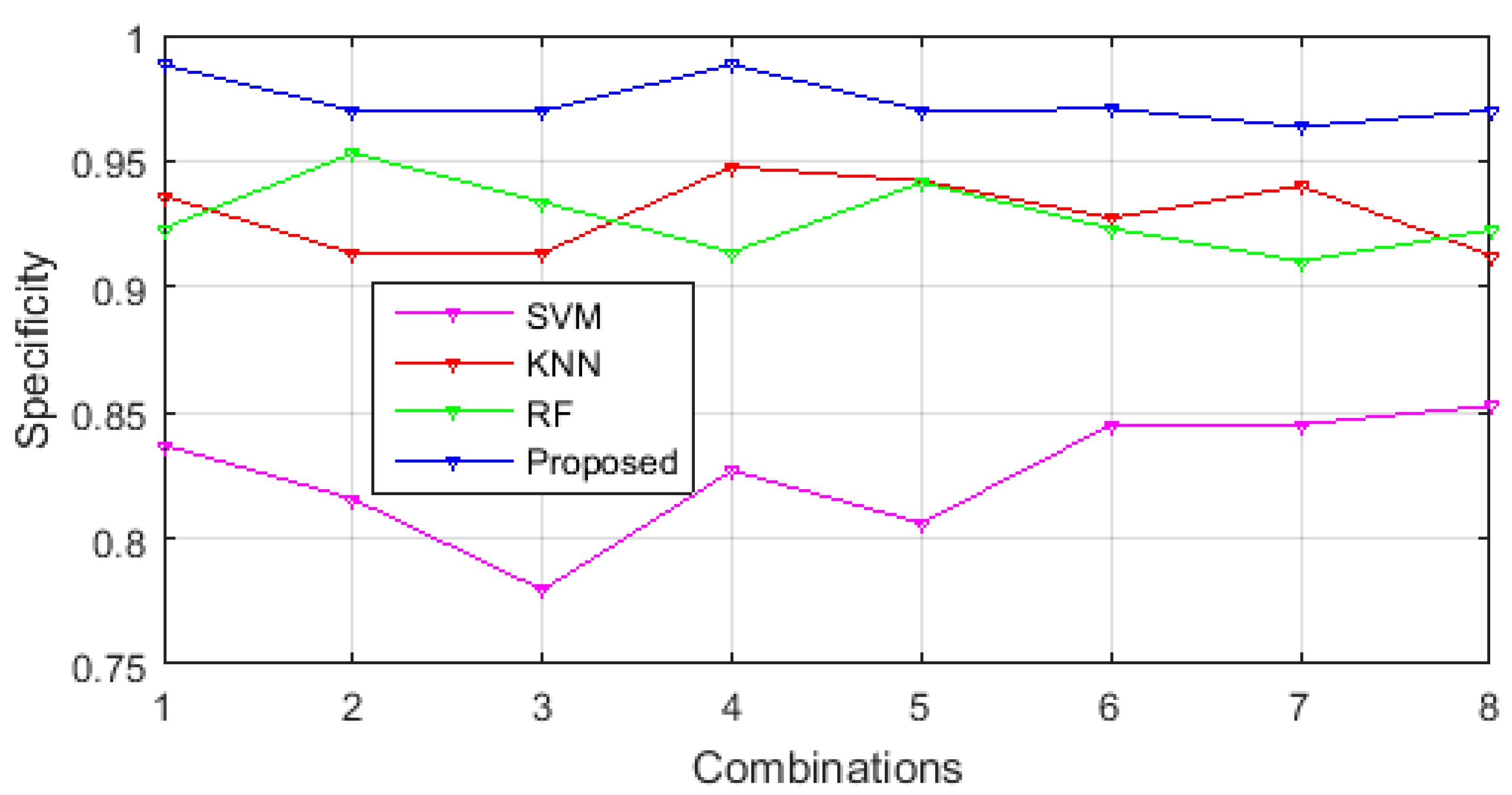
3.3. Comparison of Classification Performance

The 95% CI with the comparison of performance evaluation for classification is shown in

Table 8. Comparison of classification performance evaluation with 95% CI.

Test Class Labels	Performance Metrics	Comparative Methods
		Existing Method [43]			Existing Method [69]		Proposed Method
		PNN	LVQ	BPN	PNN	SVM	Ensemble
Fatty	Accuracy	0.76 (0.5226, 0.9170)	0.80 (0.5641, 0.9431)	0.80 (0.5641, 0.9431)	0.61 (0.3787, 0.8073)	0.85 (0.6184, 0.9733)	0.90 (0.6760, 1.0000)
	Sensitivity	0.79 (0.5536, 0.9367)	0.61 (0.3787, 0.8073)	0.65 (0.4151, 0.8382)	0.81 (0.5747, 0.9494)	0.76 (0.5226, 0.9170)	1.00 (0.8076, 1.0000)
	Specificity	0.84 (0.6073, 0.9675)	0.81 (0.5747, 0.9494)	0.81 (0.5747, 0.9494)	0.81 (0.5747, 0.9494)	0.94 (0.7253, 1.0000)	0.88 (0.6525, 0.9899)
Metastasis	Accuracy	0.95 (0.7382, 1.0000)	0.14 (0.0362, 0.3551)	0.85 (0.6184, 0.9733)	0.95 (0.7382, 1.0000)	0.95 (0.7382, 1.0000)	0.95 (0.7382, 1.0000)
	Sensitivity	0.80 (0.5641, 0.9431)	0.63 (0.3969, 0.8229)	0.67 (0.4342, 0.8532)	0.81 (0.5747, 0.9494)	0.81 (0.5747, 0.9494)	0.66 (0.4248, 0.8457)
	Specificity	0.78 (0.5431, 0.9303)	0.81 (0.5747, 0.9494)	0.81 (0.5747, 0.9494)	0.81 (0.5747, 0.9494)	0.91 (0.6880, 1.0000)	1.00 (0.8076, 1.0000)
Cancer	Accuracy	0.95 (0.7382, 1.0000)	0.90 (0.6760, 1.0000)	0.90 (0.6760, 1.0000)	0.95 (0.7382, 1.0000)	0.95 (0.7382, 1.0000)	0.95 (0.7382, 1.0000)
	Sensitivity	0.72 (0.4825, 0.8895)	0.64 (0.4061, 0.8306)	0.68 (0.4437, 0.8606)	0.83 (0.5963, 0.9616)	0.78 (0.5431, 0.9303)	0.50 (0.2834, 0.7166)
	Specificity	0.89 (0.6642, 0.9952)	0.81 (0.5747, 0.9494)	0.83 (0.5963, 0.9616)	0.83 (0.5963, 0.9616)	0.88 (0.6525, 0.9899)	1.00 (0.8076, 1.0000)
Cirrhosis	Accuracy	1.00 (0.8076, 1.0000)	0.90 (0.6760, 1.0000)	0.90 (0.6760, 1.0000)	0.95 (0.7382, 1.0000)	0.95 (0.7382, 1.0000)	1.00 (0.8076, 1.0000)
	Sensitivity	0.78 (0.5431, 0.9303)	0.61 (0.3787, 0.8073)	0.66 (0.4248, 0.8457)	0.85 (0.6184, 0.9733)	0.75 (0.5124, 0.9103)	1.00 (0.8076, 1.0000)
	Specificity	0.91 (0.6880, 1.0000)	0.79 (0.5536, 0.9367)	0.85 (0.6184, 0.9733)	0.85 (0.6184, 0.9733)	0.90 (0.6760, 1.0000)	1.00 (0.8076, 1.0000)
Normal	Accuracy	0.85 (0.6184, 0.9733)	0.52 (0.3002, 0.7337)	0.47 (0.2589, 0.6904)	0.76 (0.5226, 0.9170)	0.90 (0.6760, 1.0000)	1.00 (0.8076, 1.0000)
	Sensitivity	0.75 (0.5124, 0.9103)	0.64 (0.4061, 0.8306)	0.67 (0.4342, 0.8532)	0.85 (0.6184, 0.9733)	0.82 (0.5855, 0.9555)	1.00 (0.8076, 1.0000)
	Specificity	0.85 (0.6184, 0.9733)	0.79 (0.5536, 0.9367)	0.85 (0.6184, 0.9733)	0.85 (0.6184, 0.9733)	0.92 (0.7002, 1.000)	1.00 (0.8076, 1.0000)

. For liver disease classification, Mala et al. [43] worked with three classifiers, namely the probabilistic neural network (PNN), the learning vector quantization (LVQ) neural network, and the back propagation neural network (BPN), and Gunasundari et al. [69] worked with the PNN and the SVM classifiers.

The same set of images used in the proposed methods was also used in the different existing methods and was taken for comparison. Table 8 shows the comparison of performance metrics with the proposed and existing methods [43,69]. From the table, it is clear that the proposed methodology excels other existing methods in terms of accuracy, but it marginally lags in sensitivity for metastasis and cancer because of the limited number of data available to train the proposed model. Similarly, the specificity of fatty liver class marginally lags when compared with that of existing algorithms given in [69].

Table 9. Average performance metrics of classification performance evaluation with 95% CI.

Parameter	Solution Methods
	Existing Method [43]			Existing Method [69]		Proposed Method
	PNN	LVQ	BPN	PNN	SVM
Accuracy	0.90 (0.6760, 1.0000)	0.65 (0.4154, 0.8382)	0.79 (0.4154, 0.8382)	0.84 (0.6073, 0.9675)	0.92 (0.7002, 1.000)	0.98 (0.7786, 1.0000)
Sensitivity	0.77 (0.5328, 0.9237)	0.65 (0.4154, 0.8382)	0.69 (0.4154, 0.8382)	0.77 (0.5328, 0.9237)	0.87 (0.6410, 0.9845)	0.96 (0.7513, 1.0000)
Specificity	0.88 (0.6525, 0.9899)	0.82 (0.5855, 0.9555)	0.85 (0.6184, 0.9733)	0.83 (0.5963, 0.9616)	0.91 (0.6880, 1.0000)	0.93 (0.7126, 1.0000)

shows the averaged values of accuracy, sensitivity, and specificity, along with its 95% CI, across five different classes for the proposed method. This was compared with the existing methods in [43,69].

It is inferred from the table that the proposed methodology for CLD classification yields the best result in terms of accuracy, sensitivity, and specificity, with 95% confidence interval of (0.7786, 1.0000), (0.7513, 1.0000), and (0.7126, 1.0000), respectively.

3.4. Clinical Feasibility

With the reduction of the query computation time and as a second opinion for diagnosis, the proposed framework presents the clinical feasibility of a 3D feature based CLD classification system. However, as the data in the dataset are restricted for certain diseases, the classification results are biased towards a single class. Thus, if the dataset contains an equal number of data for each class, this would be a better diagnostic tool in radiological practices.

4. Conclusions

The CLD classification using hybrid WOA-SA and ensemble classifiers is proposed. The results experimented on 3D VOIs from clinical CT image datasets suggest the usefulness of employing WOA-SA to optimally select features for the ensemble classifier. The results show that the proposed method excelled the two discussed state-of-the-art methods by ~20% and ~10% for accuracy, ~26% and ~14% for sensitivity, and ~8% and ~6% for specificity, respectively. Another interesting result of the proposed method was the error rate, which was 1.90%, a very small number when compared to the existing methods of SVM, k-NN, and RF, which produce 17.14%, 7.62%, and 11.43% error rates, respectively.

In the future, the datasets will be expanded so as to obtain a more or less equal number of samples in each class and to develop a diagnostic system for other CLDs (apart from the four liver diseases dealt with in this paper). Also, by designing a query processing system with more pathological cases, this system can be integrated as a diagnostic assistant to the radiological practices. Moreover, although there are many types of liver disease, this conceptual classification applies to only the five chosen categories of CLD—normal liver, fatty liver, cirrhosis, metastasis, and cancerous liver. This can be expanded to apply for other CLDs in the future.

References

1. Abdar, M.; Zomorodi-Moghadam, M.; Das, R.; Ting, I.H. Performance analysis of classification algorithms on early detection of liver disease. Expert Syst. Appl. 2017, 67, 239–251. [Google Scholar] [CrossRef]
2. Gatos, I.; Tsantis, S.; Spiliopoulos, S.; Karnabatidis, D.; Theotokas, I.; Zoumpoulis, P.; Loupas, T.; Hazle, J.D.; Kagadis, G.C. A Machine-Learning Algorithm Toward Color Analysis for Chronic Liver Disease Classification, Employing Ultrasound Shear Wave Elastography. Ultrasound Med. Biol. 2017, 43, 1797–1810. [Google Scholar] [CrossRef] [PubMed]
3. Kawano, Y.; Cohen, D.E. Mechanisms of hepatic triglyceride accumulation in non-alcoholic fatty liver disease. J. Gastroenterol. 2013, 48, 434–441. [Google Scholar] [CrossRef] [PubMed] [Green Version]
4. World Health Organization. Hepatitis B. 2018. Available online: https://www.who.int/news-room/fact-sheets/detail/hepatitis-b (accessed on 14 December 2018).
5. Health24. Health Cirrhosis of the Liver. Available online: https://www.health24.com/Medical/Liver-Health/Cirrhosis-of-the-liver/Cirrhosis-of-the-liver-2012072 (accessed on 14 December 2018).
6. Liver Metastasis. Available online: https://www.healthline.com/health/liver-metastases (accessed on 14 December 2018).
7. Metastatic Cancer. Available online: http://www.cancer.ca/en/cancer-information/cancer-type/metastatic-cancer/liver-metastases/?region=on (accessed on 14 December 2018).
8. Miriam, E. Tucker The Liver Meeting 2013: American Association for the Study of Liver Diseases (AASLD). Medscape. 2013. Available online: https://www.medscape.com/viewarticle/813788 (accessed on 14 December 2018).
9. Campbell, A. Alcohol-related deaths in the UK: Registered in 2015. Available online: https://www.ons.gov.uk/peoplepopulationandcommunity/healthandsocialcare/causesofdeath/bulletins/alcoholrelateddeathsintheunitedkingdom/registeredin2015 (accessed on 12 December 2018).
10. Banerjee, R.; Pavlides, M.; Tunnicliffe, E.M.; Piechnik, S.K.; Sarania, N.; Philips, R.; Collier, J.D.; Booth, J.C.; Schneider, J.E.; Wang, L.M.; et al. Multiparametric magnetic resonance for the non-invasive diagnosis of liver disease. J. Hepatol. 2014, 60, 69–77. [Google Scholar] [CrossRef] [PubMed] [Green Version]
11. Wong, R.J.; Aguilar, M.; Cheung, R.; Perumpail, R.B.; Harrison, S.A.; Younossi, Z.M.; Ahmed, A. Nonalcoholic steatohepatitis is the second leading etiology of liver disease among adults awaiting liver transplantation in the United States. Gastroenterology 2015, 148, 547–555. [Google Scholar] [CrossRef] [PubMed]
12. Lin, S.C.; Heba, E.; Wolfson, T.; Ang, B.; Gamst, A.; Han, A.; Erdman, J.W.; O’Brien, W.D.; Andre, M.P.; Sirlin, C.B.; et al. Noninvasive Diagnosis of Nonalcoholic Fatty Liver Disease Andquantification of Liver Fat Using a New Quantitative Ultrasound Technique. Clin. Gastroenterol. Hepatol. 2015, 13, 1337–1345. [Google Scholar] [CrossRef]
13. Mauri, G.; Cova, L.; De Beni, S.; Ierace, T.; Tondolo, T.; Cerri, A.; Goldberg, S.N.; Solbiati, L. Real-Time US-CT/MRI Image Fusion for Guidance of Thermal Ablation of Liver Tumors Undetectable with US: Results in 295 Cases. CardioVascular Int. Radiol. 2015, 38, 143–151. [Google Scholar] [CrossRef]
14. Thian, Y.L.; Riddell, A.M.; Koh, D.M. Liver-specific agents for contrast-enhanced MRI: Role in oncological imaging. Cancer Imaging 2013, 13, 567–579. [Google Scholar] [CrossRef]
15. López-Mir, F.; Naranjo, V.; Angulo, J.; Alcañiz, M.; Luna, L. Liver segmentation in MRI: A fully automatic method based on stochastic partitions. Comput. Methods Programs Biomed. 2014, 114, 11–28. [Google Scholar] [CrossRef] [Green Version]
16. Kechichia, R.; Valette, S.; Desvignes, M.; Prost, R. Shortest-Path Constraints for 3D Multiobject Semiautomatic Segmentation via Clustering and Graph Cut. IEEE Trans. Image Process. 2013, 22, 4224–4236. [Google Scholar] [CrossRef]
17. Deng, J.; Fishbein, M.H.; Rigsby, C.K.; Zhang, G.; Schoeneman, S.E.; Donaldson, J.S. Quantitative MRI for hepatic fat fraction and T2* measurement in pediatric patients with non-alcoholic fatty liver disease. Pediatr. Radiol. 2014, 44, 1379–1387. [Google Scholar] [CrossRef] [PubMed]
18. Reiner, C.S.; Stolzmann, P.; Husmann, L.; Burger, I.A.; Von Schulthess, G.K.; Veit-haibach, P. Protocol requirements and diagnostic value of PET/MR imaging for liver metastasis detection. Eur. J. Nucl. Med. Mol. Imajing 2014, 41, 649–658. [Google Scholar] [CrossRef] [PubMed]
19. Ichikawa, S.; Motosugi, U.; Morisaka, H.; Sano, K.; Ichikawa, T.; Tatsumi, A.; Enomoto, N.; Matsuda, M.; Fujii, H.; Onishi, H. Comparison of the diagnostic accuracies of magnetic resonance elastography and transient elastography for hepatic fibrosis. Magn. Resonance Imaging 2015, 33, 26–30. [Google Scholar] [CrossRef] [PubMed]
20. HA, S.; AH, A.-R. Liver biopsy remains the gold standard for evaluation of chronic hepatitis and fibrosis. J. Gastrointest. Liver Dis. 2007, 16, 425–426. [Google Scholar]
21. Castera, L. Invasive and non-invasive methods for the assessment of fibrosis and disease progression in chronic liver disease. Best Pract. Res. Clin. Gastroenterol. 2011, 25, 291–303. [Google Scholar] [CrossRef] [PubMed]
22. Beuthan, J.; Minet, O.; Müller, G. Quantitative optical biopsy of liver tissue ex vivo. IEEE J. Sel. Top. Quantum Electron. 1996, 2, 906–913. [Google Scholar] [CrossRef]
23. Schuppan, D.; Afdhal, N.H. Seminar Liver cirrhosis. Lancet 2008, 371, 838–851. [Google Scholar] [CrossRef]
24. Lurie, Y.; Webb, M.; Cytter-Kuint, R.; Shteingart, S.; Lederkremer, G.Z. Non-invasive diagnosis of liver fibrosis and cirrhosis. World J. Gastroenterol. 2015, 21, 11567–11583. [Google Scholar] [CrossRef]
25. Gletsos, M.; Mougiakakou, S.G.; Matsopoulos, G.K.; Nikita, K.S.; Nikita, A.S.; Kelekis, D. A Computer-Aided Diagnostic System to Characterize CT Focal Liver Lesions: Design and Optimization of a Neural Network Classifier. IEEE Trans. Inf. Technol. Biomed. 2003, 7, 153–162. [Google Scholar] [CrossRef]
26. Xian, G.M. An identification method of malignant and benign liver tumors from ultrasonography based on GLCM texture features and fuzzy SVM. Expert Syst. Appl. 2010, 37, 6737–6741. [Google Scholar] [CrossRef]
27. Mougiakakou, S.G.; Valavanis, I.K.; Nikita, A.; Nikita, K.S. Differential diagnosis of CT focal liver lesions using texture features, feature selection and ensemble driven classifiers. Artif. Intell. Med. 2007, 41, 25–37. [Google Scholar] [CrossRef] [PubMed]
28. Haralick, R.M.; Shanmugam, K.; Dinstein, I. Textural Features for Image Classification. IEEE Trans. Syst. Man Cybernet. 1973, SMC-3, 610–621. [Google Scholar] [CrossRef]
29. Prakash, K.N.B.; Ramakrishnan, A.G.; Member, S.; Suresh, S.; Chow, T.W.P. Fetal lung maturity analysis using ultrasound image features. IEEE Trans. Inf. Technol. Biomed. 2002, 6, 38–45. [Google Scholar] [CrossRef] [PubMed]
30. Wu, C.; Chen, Y.; Member, S.; Hsieh, K. Texture Features for Classification of Ultrasonic Liver Images. IEEE Trans. Med. Imaging 1992, 11, 141–152. [Google Scholar]
31. Mohamed, S.S.; Salama, M.M.A. Computer-aided diagnosis for prostate cancer using support vector machine. Proceedings 2005, 5744, 898–906. [Google Scholar] [CrossRef]
32. Yu, H.; Caldwell, C.; Mah, K.; Mozeg, D. Coregistered FDG PET/CT-Based Textural Characterization of Head and Neck Cancer for Radiation Treatment Planning. IEEE Trans. Med. Imaging 2009, 28, 374–383. [Google Scholar]
33. Wagner, M.; Besa, C.; Ayache, J.B.; Yasar, T.K.; Bane, O.; Fung, M.; Ehman, R.L.; Taouli, B. Magnetic resonance elastography of the liver: Qualitative and quantitative comparison of gradient echo and spin echo echoplanar imaging sequences. Investig. Radiol. 2016, 51, 575–581. [Google Scholar] [CrossRef]
34. Wooden, B.; Goossens, N.; Hoshida, Y.; Friedman, S.L. Using Big Data to Discover Diagnostics and Therapeutics for Gastrointestinal and Liver Diseases. Gastroenterology 2017, 152, 53–67.e3. [Google Scholar] [CrossRef] [Green Version]
35. Liang, J.D.; Ping, X.O.; Tseng, Y.J.; Huang, G.T.; Lai, F.; Yang, P.M. Recurrence predictive models for patients with hepatocellular carcinoma after radiofrequency ablation using support vector machines with feature selection methods. Comput. Methods Programs Biomed. 2014, 117, 425–434. [Google Scholar] [CrossRef]
36. Rau, H.H.; Hsu, C.Y.; Lin, Y.A.; Atique, S.; Fuad, A.; Wei, L.M.; Hsu, M.H. Development of a web-based liver cancer prediction model for type II diabetes patients by using an artificial neural network. Comput. Methods Programs Biomed. 2016, 125, 58–65. [Google Scholar] [CrossRef]
37. Özşen, S.; Güneş, S. Attribute weighting via genetic algorithms for attribute weighted artificial immune system (AWAIS) and its application to heart disease and liver disorders problems. Expert Syst. Appl. 2009, 36, 386–392. [Google Scholar] [CrossRef]
38. Acharya, U.R.; Faust, O.; Molinari, F.; Sree, S.V.; Junnarkar, S.P.; Sudarshan, V. Ultrasound-based tissue characterization and classification of fatty liver disease: A screening and diagnostic paradigm. Knowl. Based Syst. 2015, 75, 66–77. [Google Scholar] [CrossRef]
39. Raghesh Krishnan, K.; Radhakrishnan, S. Hybrid approach to classification of focal and diffused liver disorders using ultrasound images with wavelets and texture features. IET Image Process. 2017, 11, 530–538. [Google Scholar] [CrossRef]
40. Zhou, X.; Zhang, Y.; Shi, M.; Shi, H.; Zheng, Z. Early detection of liver disease using data visualisation and classification method. Biomed. Signal Process. Control 2014, 11, 27–35. [Google Scholar] [CrossRef]
41. Chang, C.C.; Chen, H.H.; Chang, Y.C.; Yang, M.Y.; Lo, C.M.; Ko, W.C.; Lee, Y.F.; Liu, K.L.; Chang, R.F. Computer-aided diagnosis of liver tumors on computed tomography images. Comput. Methods Programs Biomed. 2017, 145, 45–51. [Google Scholar] [CrossRef] [PubMed]
42. Liang, C.; Peng, L. An automated diagnosis system of liver disease using artificial immune and genetic algorithms. J. Med. Syst. 2013, 37. [Google Scholar] [CrossRef] [PubMed]
43. Mala, K.; Sadasivam, V.; Alagappan, S. Neural network based texture analysis of CT images for fatty and cirrhosis liver classification. Appl. Soft Comput. J. 2015, 32, 80–86. [Google Scholar] [CrossRef]
44. Xu, X.; Zhang, X.; Tian, Q.; Zhang, G.; Liu, Y.; Cui, G.; Meng, J.; Wu, Y.; Liu, T.; Yang, Z.; et al. Three-dimensional texture features from intensity and high-order derivative maps for the discrimination between bladder tumors and wall tissues via MRI. Int. J. Comput. Assist. Radiol. Surg. 2017, 12, 645–656. [Google Scholar] [CrossRef]
45. Lamecker, H.; Lange, T.; Seebass, M. Segmentation of the Liver Using a 3D Statistical Shape Model; Technical Report; Zuse Institute Berlin: Berlin, Germany, 2004. [Google Scholar]
46. Badakhshannoory, H.; Member, S.; Saeedi, P. A Model-Based Validation Scheme for Organ Segmentation in CT Scan Volumes. IEEE Trans. Biomed. Eng. 2011, 58, 2681–2693. [Google Scholar] [CrossRef]
47. Zhang, X.; Tian, J.; Deng, K.; Wu, Y.; Li, X.; Construction, A.S. Automatic Liver Segmentation Using a Statistical Shape Model With Optimal Surface Detection. IEEE Trans. Biomed. Eng. 2010, 57, 2622–2626. [Google Scholar] [CrossRef]
48. Soler, L.; Delingette, H.; Malandain, G.; Montagnat, J.; Ayache, N.; Koehl, C.; Dourthe, O.; Malassagne, B.; Smith, M.; Mutter, D.; et al. Fully automatic anatomical, pathological, and functional segmentation from CT scans for hepatic surgery. Comput. Aided Surg. 2001, 6, 131–142. [Google Scholar] [CrossRef] [PubMed]
49. Beck, A.; Aurich, V. HepaTux—A Semiautomatic Liver Segmentation System. 2007. Available online: http://sliver07.org/data/2007-10-24-2338.pdf (accessed on 15 November 2018).
50. Rusko, L.; Bekes, G.; Nmeth, G.; Fidrich, M. Fully Automatic Liver Segmentation for Contrast-Enhanced CT Images. 2007. Available online: http://mbi.dkfz-heidelberg.de/grand-challenge2007/web/p143.pdf (accessed on 11 December 2018).
51. Foruzan, A.H.; Aghaeizadeh, R.; Hori, M.; Sato, Y. Liver segmentation by intensity analysis and anatomical information in multi-slice CT images. Int. J. Comput. Assist. Radiol. Surg. 2009, 4, 287–297. [Google Scholar] [CrossRef] [PubMed]
52. Tsai, D.; Tanahashi, N. Neural-Network-Based Boundary Detection of Liver Structure in CT Images for 3-D Visualization. In Proceedings of the 1994 IEEE International Conference on Neural Networks, Orlando, FL, USA, 28 June–2 July 1994; pp. 3484–3489. [Google Scholar]
53. Pham, M.; Susomboon, R.; Disney, T.; Raicu, D.; Furst, J. A Comparison of Texture Models for Automatic Liver Segmentation. 2007. Available online: https://www.spiedigitallibrary.org/conference-proceedings-of-spie/6512/1/A-comparison-of-texture-models-for-automatic-liver-segmentation/10.1117/12.710422.short?SSO=1 (accessed on 15 November 2018).
54. Heimann, T.; van Ginneken, B.; Styner, M.A.; Arzhaeva, Y.; Aurich, V.; Bauer, C.; Beck, A.; Becker, C.; Beichel, R.; Bekes, G.; et al. Comparison and Evaluation of Methods for Liver Segmentation From CT Datasets. IEEE Trans. Med. Imaging 2009, 28, 1251–1265. [Google Scholar] [CrossRef] [PubMed] [Green Version]
55. Zhang, K.; Zhang, L.; Song, H.; Zhou, W. Active contours with selective local or global segmentation: A new formulation and level set method. Image Vis. Comput. 2010, 28, 668–676. [Google Scholar] [CrossRef]
56. Tamura, H.; Mori, S.; Yamawaki, T. Textural Features Corresponding to Visual Perception. IEEE Trans. Syst. Man Cybern. 1978, 8, 460–473. [Google Scholar] [CrossRef]
57. Song, B.; Zhang, G.; Lu, H.; Wang, H.; Zhu, W.; Pickhardt, P.J. Volumetric texture features from higher-order images for diagnosis of colon lesions via CT colonography. Int. J. Comput. Assist. Radiol. Surg. 2014, 9, 1021–1031. [Google Scholar] [CrossRef] [PubMed] [Green Version]
58. King, R. Textural features corresponding to textural properties. IEEE Trans. Syst. Man Cybern. 1989, 19, 1264–1274. [Google Scholar]
59. Mirjalili, S.; Lewis, A. S-shaped versus V-shaped transfer functions for binary Particle Swarm Optimization. Swarm Evol. Comput. 2013, 9, 1–14. [Google Scholar] [CrossRef]
60. Mafarja, M.M.; Mirjalili, S. Hybrid Whale Optimization Algorithm with simulated annealing for feature selection. Neurocomputing 2017, 260, 302–312. [Google Scholar] [CrossRef]
61. Elton, R.J.; Vasuki, P.; Mohanalin, J. Voice activity detection using fuzzy entropy and support vector machine. Entropy 2016, 18, 298. [Google Scholar] [CrossRef]
62. Hwang, Y.N.; Lee, J.H.; Kim, G.Y.; Shin, E.S.; Kim, S.M. Characterization of coronary plaque regions in intravascular ultrasound images using a hybrid ensemble classifier. Comput. Methods Programs Biomed. 2018, 153, 83–92. [Google Scholar] [CrossRef] [PubMed]
63. Hashem, E.M.; Mabrouk, M.S. A Study of Support Vector Machine Algorithm for Liver Disease Diagnosis. Am. J. Intell. Syst. 2014, 4, 9–14. [Google Scholar] [CrossRef]
64. Gray, K.R.; Aljabar, P.; Heckemann, R.A.; Hammers, A.; Rueckert, D. Random forest-based similarity measures for multi-modal classification of Alzheimer’s disease. NeuroImage 2013, 65, 167–175. [Google Scholar] [CrossRef] [PubMed]
65. Lam, L.; Suen, C.Y.; Ieee, F. Application of Majority Voting to Pattern Recognition: An Analysis of Its Behavior and Performance. IEEE Trans. Syst. Man Cybern. Part A Syst. Hum. 1997, 27, 553–568. [Google Scholar] [CrossRef]
66. Linguraru, M.G.; Richbourg, W.J.; Liu, J.; Watt, J.M.; Pamulapati, V.; Wang, S.; Summers, R.M. Tumor burden analysis on computed tomography by automated liver and tumor segmentation. IEEE Trans. Med. Imaging 2012, 31, 1965–1976. [Google Scholar] [CrossRef]
67. Deng, X.; Du, G. 3D Segmentation in the Clinic: A Grand Challenge II—Liver Tumor Segmentation. 2008. Available online: http://www.midasjournal.org/browse/journal/45 (accessed on 22 October 2018).
68. Hossin, M.; Sulaiman, M. A review on evaluation metrics for data classification evaluations. Int. J. Data Min. Knowl. Manag. Process 2015, 5, 1–11. [Google Scholar]
69. Gunasundari, S.; Janakiraman, S.; Meenambal, S. Velocity Bounded Boolean Particle Swarm Optimization for improved feature selection in liver and kidney disease diagnosis. Expert Syst. Appl. 2016, 56, 28–47. [Google Scholar] [CrossRef]
Figure 1. Block diagram of the proposed liver disease classification.
Symmetry 11 00033 g001
Figure 2. (a,g) Raw clinical CT slice; (b,h) segmented CT slice; (c,i) referential boundary detection; volume extraction of liver in (d,j) bottom view; (e,k) straight view; (f,l) top view.
Symmetry 11 00033 g002
Figure 3. Accuracy comparison of ensemble classifier with 3D feature-set combinations.
Symmetry 11 00033 g003
Figure 4. Sensitivity comparison of ensemble classifier with 3D feature-set combinations.
Symmetry 11 00033 g004
Figure 5. Specificity comparison of ensemble classifier with 3D feature-set combinations.
Symmetry 11 00033 g005
Figure 6. Box plot of performance metrics for CLD classification in terms of accuracy, sensitivity, and specificity.
Symmetry 11 00033 g006
Figure 7. Confusion matrix of liver classification.
Symmetry 11 00033 g007