Article

A New Pairwise NPN Boolean Matching Algorithm Based on Structural Difference Signature

1
The School of Computer Science and Engineering, University of Xinjiang Finance and Economics, Urumqi 830012, China
2
The Big Data Research Center, School of Computer Science and Engineering, University of Electronic Science and Technology of China, Chengdu 611731, China
3
Guangxi Key Laboratory of Hybrid Computation and IC Design Analysis, Guangxi University for Nationalities, Nanning 530006, China
4
Synopsys Inc., Mountain View, CA 94043, USA
5
The School of Computer and Electronic Information, Guangxi University, Nanning 530004, China
6
Network and Data Security Key Laboratory of Sichuan Province, University of Electronic Science and Technology of China, Chengdu 611731, China
*
Authors to whom correspondence should be addressed.
Symmetry 2019, 11(1), 27; https://doi.org/10.3390/sym11010027
Submission received: 21 September 2018 / Revised: 11 December 2018 / Accepted: 21 December 2018 / Published: 29 December 2018

Abstract

:
In this paper, we address an NPN Boolean matching algorithm. The proposed structural difference signature (SDS) of a Boolean function significantly reduces the search space in the Boolean matching process. The paper analyses the size of the search space from three perspectives: the total number of possible transformations, the number of candidate transformations and the number of decompositions. We test the search space and run time on a large number of randomly generated circuits and Microelectronics Center of North Carolina (MCNC) benchmark circuits with 7–22 inputs. The experimental results show that the search space of Boolean matching is greatly reduced and the matching speed is obviously accelerated.

1. Introduction

Boolean equivalence classification and matching constitute a long-standing and open problem. The authors of [1,2] applied a group algebraic approach to NP and NPN Boolean equivalence classification. Reference [2] computed the classification results for 10 inputs. Affine equivalence classification is also an important field of study with applications in logic synthesis and cryptography [3]. All Boolean functions in an equivalence class are equivalent to each other. NPN Boolean matching determines whether two Boolean functions are equivalent under input negation and/or permutation and/or output negation. This paper studies NPN Boolean matching for single-output completely specified Boolean functions.
NPN Boolean matching is an important research topic that can be applied to a number of applications in integrated circuit design, such as technology mapping, cell library binding and logic verification [4]. When a Boolean circuit is functionally NPN-equivalent to another Boolean circuit, one of these circuits can be realized by means of the other. There are n ! 2 n + 1 NPN transformations for a n-variable Boolean function. If Boolean function f is NPN-equivalent to Boolean function g, there must be a NPN transformation that can transform f to g. On the contrary, no NPN transformation can transform f to g. The purpose of our proposed algorithm is to find the NPN transformation that can transform Boolean function f to g as early as possible. Based on the structural signature (SS) vector in our previous study [5], we proposes a new combined signature vector, i.e., SDS vector. In this paper, Boolean difference sigture is introduced into SS vector to form SDS vector. The new signature vector SDS is better able to distinguish variables and reduce the research space for NPN Boolean matching. Experimental results show that the search space is reduced by more than 48% compared with [5] and that the run time of our algorithm is reduced by 42% and 80% compared with [5,6], respectively.
In the following, Section 2 introduces relevant works on NPN-equivalence matching. Section 3 introduces some terminology and notation. Section 4 describes the proposed algorithm in detail. In Section 5, we present experimental results to demonstrate the effectiveness of our algorithm. Section 6 concludes the paper.

2. Related Works

Many methods can be exploited to solve the problem of NPN Boolean matching. The main results of such research are focused on four methods: (1) algorithms on canonical forms; (2) pairwise matching algorithms using signatures; (3) algorithms based on satisfiability (SAT) and (4) algorithms based on spectral analysis.
Each method has its own advantages. In canonical-form-based matching algorithms, the canonical form of each Boolean circuit of cell library is stored in advance. When cell-library binding is implemented, the canonical form of each Boolean circuit to be matched is computed and compared with the canonical forms of each Boolean circuits in the cell library via a hash table. All Boolean functions in an equivalence class have the same canonical form. The canonical form of each equivalence class has a special value. References [6,7,8,9,10,11,12] studied Boolean matching based on canonical forms and attained significant achievements.
Reference [12] reported P-equivalence matching for 20-input Boolean functions. The canonical forms considered in reference [12] was the binary strings with the maximal scores in lexicographic comparison. Reference [7] devised a procedure to canonicalize a threshold logic function and judged equivalence of two threshold logic functions by their canonicalized linear inequalities. Based on the canonical form of Boolean function, the reference [8] reduced the number of configuration bits in an FPGA architecture. The authors of [10,11] proposed fast Boolean matching based on NPN Boolean classification; their canonical form has the maximal truth table. The authors of [6] proposed new canonical forms based on signatures.
A pairwise matching algorithm searches the NPN transformations between two Boolean functions using signatures, which is a semi-exhaustive search algorithm. The merit of this method is that once it finds a transformation that can prove the equivalence of two Boolean functions, other transformations will not be checked. The authors of [4,5,13,14] proposed Boolean matching algorithms based on pairwise matching and used binary decision diagrams (BDDs) to represent Boolean functions. The authors of [5] proposed a structural signature vector to search the transformations between two Boolean functions and implemented NPN Boolean matching for 22 inputs. In pairwise matching algorithms, signatures are usually used as a necessary condition for judging whether two Boolean functions are equivalent, and variable symmetry is commonly utilized to reduce the search space. Symmetric attributes are used in many fields. Reference [15] studied the symmetries of the unitary Lie group. The variable symmetric attributes of Boolean function are widely used in NPN Boolean equivalence matching. In reference [5], the search space was reduced and the matching speed was improved by means of structural signatures, variable symmetry, phase collision check and variable grouping.
Since a SAT solver can help solve the problem of NPN Boolean matching and because many quick SAT solvers can be utilized, many Boolean matching algorithms based on SAT have emerged in recent years. The authors of [16,17,18,19,20] studied SAT-based Boolean matching. Based on graphs, simulation and SAT, Matsunaga [16] achieved PP-equivalence Boolean matching with larger inputs and outputs. The authors of [17,18] studied Boolean matching for FPGAs utilizing SAT technology. Cong et al. [19] used the implicant table to derive the SAT formulation and achieved significant improvements. The authors of [20] combined simulation and SAT to perform P-equivalent Boolean matching for large Boolean functions. Compared with studies based on the previous three methods, studies on Boolean matching that use spectral techniques are fewer in number. Moore et al. [21] presented an NPN Boolean matching algorithm using Walsh spectra. The authors of [22] utilized Haar spectra to check the equivalence of two logic circuits.
Regardless of which method is used, the key to Boolean matching is to reduce the search space. It is universally known that the search space for exhaustive NPN Boolean matching is O ( n ! 2 n + 1 ) . In the methods discussed above, many strategies are used to reduce the search space. The authors of [6] used general signatures and symmetry to reduce the search space.
Based on our previous study [5], we propose a new combined signature, i.e., the structural difference signature. We present a new pairwise algorithm based on the following conditions: (1) two NP-equivalent Boolean functions have the same SDS vectors; (2) two variables of a variable mapping have the same SDS values; and (3) two groups of Boolean functions Shannon decomposed with splitting variables are NP-equivalent.

3. Terminology and Notation

Let f ( x 0 , x 1 , , x n 1 ) and g ( x 0 , x 1 , , x n 1 ) be two single-output completely specified Boolean functions. The problem to be solved in this paper is to determine whether f is NPN-equivalent to g. Some related terminology has been introduced in [5,6].
An NP transformation T is composed of input negations and/or permutations. It can also be expressed as a group of variable mappings. In reference [5], the mapping from the variable x i of f to the variable x j of g, φ i , can be classified into two cases: (1) x i maps to x j with the same phase, in which case the mapping is x i x j or x ¯ i x ¯ j ; or (2) x i maps to x j with the opposite phase, in which case the mapping is x i x ¯ j or x ¯ i x j . A same-phase relation indicates no input negation, whereas an opposite-phase relation indicates input negation. A same-phase variable mapping between the variables x i and x j is abbreviated as i j 0 , and an opposite-phase variable mapping between the variables x i and x j is abbreviated as i j 1 . For two NPN-equivalent Boolean functions f and g, there may be an output negation when f = g ¯ .
Definition 1.
(NPN equivalence) Two Boolean functions f and g are NPN equivalent, f g , if and only if there exists an NP transformation T that satisfies f ( T X ) = g ( X ) or f ( T X ) = g ( X ) ¯ .
As a general signature, the cofactor signature is widely applied in NPN Boolean matching. The cofactor signature of f ( X ) with respect to x i ( x ¯ i ) is f x i ( f x ¯ i ) [5].
Reference [5] proposed SS vector. The SS value of f with respect to x i , V i , is ( f x i , f x ¯ i , C i , C i , G i ) . ( f x i , f x ¯ i ) is the 1st signature of the variable x i , and C i and | C i | are the symmetry mark, and G i is group mark. According to their symmetry properties, the variables of a Boolean function are classified as either asymmetric and symmetric. An asymmetric variable may have a single-mapping set or a multiple-mapping set. The variable mapping set of the asymmetric variable x i is denoted by χ i . Similarly, a symmetric variable may have a single symmetry-mapping set or a multiple symmetry-mapping set. The symmetry-mapping set of the symmetry class C i is denoted by S i , and the symmetry mapping between C i and C j is denoted by C i C j . The literal ψ i represents a group of two or more variable mappings generated by C i C j .
A P transformation does not change the cofactor signature of a variable. However, an N transformation changes the order of the positive and negative cofactor signatures without changing their numerical values. Therefore, we do not consider the order of the positive and negative cofactor signatures when comparing the 1st signature values of two variables. A variable x i may be transformed into an arbitrary variable x j , 0 j n 1 ; therefore, we also do not consider the order of the variables when we compare two SS vectors.
Given two NP-equivalent Boolean functions f and g with a variable mapping x i x j between them, we have the following four facts: (1) V f = V g and V i = V j ; (2) The Boolean functions decomposed with x i and x j using the Shannon expansion must be NP equivalent. Specifically, x i f x i is NP equivalent to x j g x j , and x ¯ i f x ¯ i is NP equivalent to x ¯ j g x ¯ j ; (3) x i and x j are either both asymmetric variables or both symmetric variables; (4) If there is a variable mapping between x l of f and x h of g, then the SS values of x l must be the same as those of x h no matter how many times the Boolean functions f and g are decomposed [5].
Two Boolean functions f and g may undergo one or more transformations in the process of matching. A transformation consists of n variable mappings. The algorithm of [5] and the algorithm presented in this paper detect all possible transformations between f and g according to their SS and SDS vectors, respectively.

4. The Proposed Algorithm

The goal of the proposed algorithm is to reduce the size of the search space as much as possible, thereby improving the speed of NPN Boolean matching.

4.1. Boolean Difference

For n inputs, there are 2 2 n different Boolean functions. Many Boolean functions have one or more independent variables. Whether a variable x i of f is independent can be determined using cofactors.
The Boolean difference of a Boolean function f with respect to x i , f x i , is the Boolean function f x i f x ¯ i , where f x i = f [ x i 1 ] and f x ¯ i = f [ x i 0 ] [23].
Definition 2.
(Boolean difference signature) The Boolean difference signature of a Boolean function f with respect to x i , | f x i | , is the number of minterms of f x i .
When a variable x i of f is NP transformed into x j ( x ¯ j ) , its Boolean difference signature does not change. Thus, Boolean difference signature, like cofactor signature, can be used to distinguish variables.
Example 1.
Consider an 5-input Boolean function f ( X ) = x 0 x ¯ 2 x ¯ 3 + x ¯ 0 x 1 x 2 x ¯ 3 + x 0 x 1 x 3 x 4 + x ¯ 0 x ¯ 1 x 3 x ¯ 4 + x 0 x ¯ 1 x ¯ 3 x ¯ 4 + x 0 x 2 x 3 x 4 + x ¯ 0 x ¯ 1 x ¯ 2 x 3 + x ¯ 0 x 2 x ¯ 3 x 4 + x 0 x 1 x 2 x 3 + x ¯ 0 x ¯ 2 x 3 x ¯ 4 . Let us compute the 1st signature and the Boolean difference signature of each variable.
The 1st signatures of x 0 , x 1 , x 2 , x 3 and x 4 are ( 9 , 7 ) , ( 8 , 8 ) , ( 8 , 8 ) , ( 8 , 8 ) and ( 8 , 8 ) , respectively. The variable x 1 is symmetric to x 4 . The Boolean difference signatures of the variables are 32, 12, 20, 28 and 12, respectively. From the 1st signatures and a symmetry check, we can distinguish variables x 0 , x 1 and x 4 . Variables x 2 and x 3 are both asymmetric variables and have the same 1st signature values. If we only utilize on their 1st signatures, the variables x 2 and x 3 cannot be distinguished. However, these two variables have different Boolean difference signatures. Thus, the variables x 2 and x 3 are actually different and can be distinguished.
Definition 3.
(Independent variable) A variable x i of a Boolean function f is an independent variable if it satisfies | f x i | = 0 .
NP transformations do not change the independence of a variable. Thus, an independent variable is still an independent variable after NP transformation.
Definition 4.
(Independent-variable set) The independent-variable set of a Boolean function f, D f , is a set that consists of all independent variables of f.
Lemma 1.
Two NPN-equivalent Boolean functions f and g have the same number of independent variables.
Proof. 
If the Boolean function f is NPN-equivalent to g, then f and g are in the same NPN equivalence class. There must exist an NP transformation T that can transform f into g or g ¯ . After NP transformation, an independent variable is still an independent variable. Therefore, it can be deduced that f and g have the same number of independent variables. □
Property 1.
The cofactor signature of a Boolean function f with respect to its variable x i is f x i = f x ¯ i = 1 2 f when the variable x i is an independent variable.
Proof. 
Since f x i = f x i f x ¯ i and | f x i | = 0 and | f x i | + | f x ¯ i | = | f | , it holds that f x i = f x ¯ i = 1 2 f . □
Because the positive cofactor signature is the same as the negative cofactor signature for an independent variable, the phases of independent variables cannot determined by using the phase assignment method presented in [5,6]. However, independent variables have no influence on a Boolean function. Thus, the proposed algorithm assigns a positive phase to all independent variables.
Example 2.
Consider two 6-input Boolean functions f ( X ) = x ¯ 0 x 1 x ¯ 2 + x ¯ 0 x 1 x 2 x 3 + x 0 x ¯ 1 x ¯ 2 + x 0 x ¯ 1 x 2 x 3 and g ( X ) = x ¯ 0 x ¯ 1 x ¯ 3 x 4 + x ¯ 0 x 1 x 3 x 4 + x 0 x ¯ 1 x ¯ 3 + x 0 x 1 x 3 . Let us compute the SS vectors, Boolean difference signatures and independent-variable sets.
The SS vectors of f and g are as follows:
V f = { ( 12 , 12 , 2 , 0 , 1 ) , ( 12 , 12 , 2 , 0 , 1 ) , ( 8 , 16 , 2 , 2 , 0 ) , ( 16 , 8 , 2 , 2 , 0 ) , ( 12 , 12 , 2 , 4 , 1 ) , ( 12 , 12 , 2 , 4 , 1 ) } ,
V g = { ( 16 , 8 , 2 , 0 , 0 ) , ( 12 , 12 , 2 , 1 , 1 ) , ( 12 , 12 , 2 , 2 , 1 ) , ( 12 , 12 , 2 , 1 , 1 ) , ( 16 , 8 , 2 , 0 , 0 ) , ( 12 , 12 , 2 , 2 , 1 ) } .
The Boolean difference signatures of the variables of f are 48, 48, 16, 16, 0 and 0. The Boolean difference signatures of the variables of g are 16, 48, 0, 48, 16 and 0. The independent-variable sets of f and g are D f = { x 4 , x 5 } and D g = { x 2 , x 5 } .
Definition 5.
(Independent mapping set) The independent mapping set between Boolean functions f and g is D = { φ i : x i x j | x i D f , x j D g } .
Consider two NP-equivalent Boolean functions f and g with independent-variable sets of D f = { x i 1 , x i 2 , x i k } and D g = { x j 1 , x j 2 , x j k } , respectively. If we do not consider the symmetry and independence of variables, then there are 2 k k ! groups of different variable mappings between D f and D g according to their 1st signatures. However, according to the properties of independent variables, we need to consider only the positive phase and create one independent-mapping set { x i 1 x j 1 , x i 2 x j 2 , x i k x j k } . Therefore, the search space is reduced significantly if there are independent variables in the Boolean functions.
In Example 2, the Boolean function f has the three symmetry classes C 0 = { x 0 , x 1 } , C 2 = { x 2 , x 3 } and C 4 = { x 4 , x 5 } , and the Boolean function g has the three symmetry classes C 0 = { x 0 , x 4 } , C 1 = { x 1 , x 3 } and C 2 = { x 2 , x 5 } if we do not consider the Boolean difference signatures. The symmetry class C 0 of f can be mapped to the symmetry classes C 1 and C 2 of g using the method of reference [5]. In other words, the symmetry classes C 0 and C 4 of Boolean function f cannot be distinguished. However, the variables in C 0 and C 4 of Boolean function f have different Boolean difference signatures. Thus, if we consider the Boolean difference signatures when searching the variable mappings, the symmetry class C 0 of f can be mapped only to the symmetry class C 1 of g, and the symmetry class C 4 of f can be mapped only to the symmetry class C 2 of g. There exists an independent-mapping set { x 4 x 2 , x 5 x 5 } .
Definition 6.
(Structural difference signature vector) An n-input Boolean function f has a structural difference signature (SDS) vector V f = { V 0 , V 1 , , V n 1 } , where V i = ( f x i , f x ¯ i , C i , C i , G i , | f x i | ) .
The algorithm presented in [5] groups variables by their 1st signature values. The algorithm proposed in this paper groups variables by their 1st signature values and Boolean difference signatures. We define the ’<’ relation between x i and x j as follows.
Definition 7.
(<) The variables x i and x j have the relation x i < x j if one of the following two cases is satisfied: (1) ( f x i , f x ¯ i ) < ( f x j , f x ¯ j ) or (2) ( f x i , f x ¯ i ) = ( f x j , f x ¯ j ) f x i < f x ¯ i .
The group numbers of the variables are generated with the above ’<’ relation. The SDS vectors of f and g in example 2 are as follows: V f = { ( 12 , 12 , 2 , 0 , 1 , 48 ) , ( 12 , 12 , 2 , 0 , 1 , 48 ) , ( 8 , 16 , 2 , 2 , 0 , 16 ) , ( 16 , 8 , 2 , 2 , 0 , 16 ) , ( 12 , 12 , 2 , 4 , 2 , 0 ) , ( 12 , 12 , 2 , 4 , 2 , 0 ) } and V g = { ( 16 , 8 , 2 , 0 , 0 , 16 ) , ( 12 , 12 , 2 , 1 , 1 , 48 ) , ( 12 , 12 , 2 , 2 , 2 , 0 ) , ( 12 , 12 , 2 , 1 , 1 , 48 ) , ( 16 , 8 , 2 , 0 , 0 , 16 ) , ( 12 , 12 , 2 , 2 , 2 , 0 ) } . In the process of grouping variables of Boolean function f, we first compare their 1st signature and do not consider the order of positive and negative cofactor signature. Therefore, variables x 2 and x 3 are grouped into group 0. The varibales in symmetry class C 0 and C 4 have the same 1st signature, so we compare their Boolean difference signature. Because the Boolean difference signature of variables in C 0 is greater than that of variables in symmetry class C 4 , the group number of variables x 0 and x 1 are 1 and the group number of variables x 4 and x 5 are 2.
The SDS vector is a new signature vector that consists of the SS vector plus a Boolean difference mark. The variable mapping search and the transformation detection of our algorithm are based on two facts: (1) two NP-equivalent Boolean functions have the same SDS vectors; and (2) there exists a possible variable mapping between the variables x i and x j if they have the same SDS values.

4.2. SDS-Based Boolean Matching Algorithm

NPN Boolean matching is defined as follows:
Given two Boolean functions f and g, if there exists an NP transformation T that satisfies f ( T X ) = g ( X ) or f ( T X ) = g ( X ) ¯ , then f is NPN-equivalent to g.
Before searching the variable mappings, the proposed algorithm first determines whether there is an output negation for Boolean function f. If there is, then our algorithm will match f and g ¯ . The method of identifying the presence of an output negation is the same as that in reference [5]. If | f | = | g | | f | | g ¯ | , then there is no output negation. There is an output negation if | f | | g | | f | = | g ¯ | . There is a tie if | f | = | g | | f | = | g ¯ | . Our algorithm handles first the condition without output negation and then the condition with output negation if f is not NP equivalent to g.
The algorithm will terminate when it finds a transformation T that satisfies f ( T X ) = g ( X ) ( g ( X ) ¯ ) or when all candidate transformations have been checked and found not to satisfy f ( T X ) = g ( X ) ( g ( X ) ¯ ) . The algorithm will attempt all possible variable mappings, and thus, it will certainly find an NP transformation T between two NP-equivalent Boolean functions f and g ( g ¯ ) .
The pseudo-code for NPN Boolean matching is given in Procedure 1.
In Procedure 1, t r a n s _ l i s t is a tree that stores the NP transformations generated in the process of transformation detection. A candidate transformation is an unabridged branch in t r a n s _ l i s t . s p _ f and s p _ g are the decomposition expressions for f and g, respectively. After the existence of an output negation has been determined, Procedure 1 calls Handle_SDS() to detect the NP transformations between f and g ( g ¯ ) and judge the NP equivalence of f and g ( g ¯ ) .
Any one NP transformation between the Boolean functions f and g ( g ¯ ) is composed of n variable mappings. Thus, the proposed algorithm searches variable mappings and generates NP transformations. In this paper, the necessary condition for two Boolean functions to be judged NP equivalent is that they must have the same SDS vector. For a variable mapping to be established between x i and x j , these two variables must satisfy the following conditions:
(1) x i and x j have the same 1st signature values, i.e., ( | f x i | , | f x ¯ i | ) = ( | f x j | , | f x ¯ j | ) ( | f x i | , | f x ¯ i | ) = ( | f x ¯ j | , | f x j | ) .
(2) x i and x j have the same Boolean difference signature, i.e., | f x i | = | f x j | .
(3) x i and x j have the same symmetry class cardinality, i.e., | C i | = | C j | .
(4) x i and x j have the same group number, i.e., G i = G j .
Procedure 1 NPN Boolean Matching.
Input:f and g
Output: 0 or 1
function Matching( f , g )
  Create BDD of f and g
   s p _ f = b d d t r u e , s p _ g = b d d t r u e , t r a n s _ l i s t = N U L L
  Compute | f | and | g |
  if | f | = | g | then
   if | f | | g ¯ | then
    Return Handle_SDS( f , g )
   else
    if Handle_SDS( f , g )=1 then
     Return 1
    else
     Return Handle_SDS(f, g ¯ )
    end if
   end if
  else
   if | f | = | g ¯ | then
    Return Handle_SDS(f, g ¯ )
   else
    Return 0
   end if
  end if
end function
In the process of the variable mapping search, Handle_SDS() searches the variable mappings for each variable that has not been identified. A variable is identified when its phase and variable mappings are determined in a transformation. After searching all variable mapping sets, Handle_SDS() selects the minimal variable mapping set to handle. The minimal variable mapping set is the one with the lowest cardinality. There are eight possible cases for the variable mapping set of the variable x i of f, as follows.
(1) The variable x i is an asymmetric variable. The phase of x i is determined, and there is only one variable x j of g that has the same SDS values as those of x i . The variable mapping set of x i is a single-mapping set. χ i = { i j k } , k { 0 , 1 } , and | χ i | = 1 .
(2) The variable x i is an asymmetric variable. There exist multiple variables x j 1 , x j 2 , , x j m of g, where m 2 , that have the same SDS values as those of x i , and their phases are determined. The variable mapping set of x i is a multiple-mapping set. χ i = { i j 1 k 1 , i j 2 k 2 , , i j m k m } , where k 1 , k 2 , , k m { 0 , 1 } , and | χ i | = m .
(3) The variable x i is an asymmetric variable. There exist one or more variables x j 1 , x j 2 , , x j m of g, where m 1 , that have the same SDS values as those of x i , and their phases are not determined. The variable mapping set of x i is a multiple-mapping set. χ i = { i j 1 0 , i j 1 1 , i j 2 0 , i j 2 1 , , i j m 0 , i j m 1 } , and | χ i | = 2 m .
(4) The variable x i is a symmetric variable, and its symmetry class is C i = { x i , x i 1 , x i 2 , , x i m 1 } . There exists only one symmetry class C j = { x j , x j 1 , x j 2 , , x j m 1 } of g whose variables have the same SDS values as those of the variables in C i , where | C i | = | C j | , and the phase of x i is determined. The variable mapping set of x i , S i , is a single symmetry-mapping set, i.e., | S i | = 1 . There exists one group of variable mappings { i j k , i 1 j 1 k 1 , i 2 j 2 k 2 , , i m 1 j m 1 k m 1 } , where k , k 1 , k 2 , , k m 1 { 0 , 1 } , between C i and C j .
(5) The variable x i is a symmetric variable, and its symmetry class is C i = { x i , x i 1 , x i 2 , , x i m 1 } . There is only one symmetry class C j = { x j , x j 1 , x j 2 , , x j m 1 } of g whose variables have the same SDS values as those of the variables in C i , where | C i | = | C j | , and the phase of x i is not determined. The variable mapping set of x i , S i , is a multiple symmetry-mapping set: | S i | = 2 . There are two groups of variable mappings, { i j 0 , i 1 j 1 k 1 , i 2 j 2 k 2 , , i m 1 j m 1 k m 1 } , where k 1 , k 2 , , k m 1 { 0 , 1 } , and { i j 1 , i 1 j 1 p 1 , i 2 j 2 p 2 , , i m 1 j m 1 p m 1 } , where p 1 , p 2 , , p m 1 { 0 , 1 } , between C i and C j .
When the variable symmetry is checked, the phase relation between two symmetric variables is known. The variable mapping relations between C i and C j can be generated in the following way.
We first consider the case in which x i and x j have the same phase, i.e., there exists a variable mapping i j 0 . A variable mapping i 1 j 1 0 exists in two cases: (1) x i is symmetric to x i 1 and x j is symmetric to x j 1 or (2) x i is symmetric to x ¯ i 1 and x j is symmetric to x ¯ j 1 . A variable mapping i 1 j 1 1 exists in two cases: (1) x i is symmetric to x i 1 and x j is symmetric to x ¯ j 1 or (2)  x i is symmetric to x ¯ i 1 and x j is symmetric to x j 1 . Then, we consider the case in which x i and x j have the opposite phase, i.e., there exists a variable mapping i j 1 . A variable mapping i 1 j 1 1 exists in two cases: (1)  x i is symmetric to x i 1 and x j is symmetric to x j 1 or (2) x i is symmetric to x ¯ i 1 and x j is symmetric to x ¯ j 1 . A variable mapping exists i 1 j 1 0 in two cases: (1) x i is symmetric to x i 1 and x j is symmetric to x ¯ j 1 or (2) x i is symmetric to x ¯ i 1 and x j is symmetric to x j 1 . Thus, two groups of variable mappings between C i and C j will be generated via this method.
(6) The variable x i is a symmetric variable, and its symmetry class is C i . There exist multiple symmetry classes C j 1 , C j 2 , , C j m , where 2 m n 2 , whose variables have the same SDS values as the variables in C i , where | C i | = | C j 1 | = | C j 2 | = = | C j m | , and the phase of x i is determined. The variable mapping set of x i , S i , is a multiple symmetry-mapping set: | S i | = m . There exists one group of variable mappings between C i and each C j p , where p { 1 , 2 , , m } .
(7) The variable x i is a symmetric variable, and its symmetry class is C i . There exist one or more symmetry classes C j 1 , C j 2 , , C j m , where 1 m n 2 , whose variables have the same SDS values as those of the variables of C i , where | C i | = | C j 1 | = | C j 2 | = = | C j k | , and the phase of x i is not determined. The variable mapping set of x i , S i , is a multiple symmetry-mapping set: | S i | = 2 m . There exist two groups of variable mappings between C i and each C j p , where p { 1 , 2 , , m } .
(8) The variable x i is an independent variable. The variable mapping set of x i is an independent mapping set.
All possible variable mapping sets are listed above. To generate an NP transformation, n variable mappings are needed for x 1 , x 2 , , x n . Each node in the NP transformation tree, t r a n s _ l i s t , represents a variable mapping, and all nodes in a given layer belong to the same variable mapping set. The methods for handling the variable mapping sets are as follows.
(1) If it is the first computation of SDS vectors, a check for independent variables is performed. If there are one or more independent variables, an independent-mapping set is created and added to t r a n s _ l i s t , and the minimal variable mapping set is then sought among the remaining variables. If there are no independent variables, Handle_SDS() searches the variable mapping sets for all variables.
(2) If the current variable mapping set of x i is a single-mapping set, our algorithm adds the variable mapping in χ i to t r a n s _ l i s t . The variable x i is identified.
(3) If the current variable mapping set of x i is a single symmetry-mapping set and x i belongs to C i , where | C i | = m , then the group ψ i of variable mappings of S i is added to t r a n s _ l i s t . To the NP transformation tree, m layers are added, where each layer contains a variable mapping node. The variables in the symmetry class C i are all identified.
(4) If the current variable mapping set of x i is a multiple-mapping set or a multiple symmetry-mapping set, then the cardinalities of the variable mapping sets are computed, and the minimal variable mapping set is recorded.
After searching all variable mapping sets, as in reference [5], our algorithm updates the two decomposition expressions s p _ f and s p _ g in the case of a single-mapping set or a single symmetry-mapping set. Otherwise, our algorithm handles the minimal variable mapping set. If the cardinality m of the minimal variable mapping set satisfies m 2 , then m branches will be generated in t r a n s _ l i s t . Each branch is handled in order.
The purpose of Procedure 2 is to search the variable mappings for all possible NP transformations. In the process of recursive_search, Procedure 2 uses the same methods applied in [5] to find and prune error NP transformation branches. That is, the current branch will be pruned if the two SDS vectors are not the same or if the current variable mapping has a phase collision.
The pseudo-code for Procedure 2 is as follows.
Procedure 2 recursive_search.
Input:f, g, s p _ f , s p _ g , and t r a n s _ l i s t
Output: 0 or 1
function handle_SDS( f , g , s p _ f , s p _ g , t r a n s _ l i s t )
  if D 1 then
   return VERIFY( f , g , T )
  end if
  UPDATE( f , g , s p _ f , s p _ g )
  if V f V g then
   return 0
  end if
  if D 2 then
   Compute D f and D g
   if N o t E m p t y ( D f ) then
    Add independent mappings to t r a n s _ l i s t
   end if
  end if
   m i n _ n u m b e r =32768
  for all x i f ( x ) do
   if D 3 then
    Continue
   end if
   for all x j g ( x ) do
    Search variable mappings
   end for
   Compute χ i ( S i )
   if D 4 then
    for all φ j ( ψ j ) χ i ( S i ) do
     if D 5 then
      return 0
     else
      Add φ j ( ψ j ) to t r a n s _ l i s t
     end if
    end for
     m i n _ n u m b e r = 1
   else
    if | χ i | ( | S i | ) < m i n _ n u m b e r then
       m i n = i
    end if
   end if
  end for
  if D 6 then
   Update s p _ f and s p _ g
   Return Handle_SDS( f , g , s p _ f , s p _ g , t r a n s _ l i s t )
  else
   for all φ j ( ψ j ) χ m i n ( S m i n ) do
    if D 5 then
     continue
    else
     Add φ j ( ψ j ) to t r a n s _ l i s t
     Update s p _ f and s p _ g
     Return Handle_SDS( f , g , s p _ f , s p _ g , t r a n s _ l i s t )
    end if
   end for
   Return 0
  end if
end function
The meanings of conditions D 1 , D 2 , D 3 , D 4 , D 5 and D 6 and the operations that need to be performed when these conditions are satisfied are defined as follows:
D 1 : When D 1 is true, a candidate transformation is generated. Procedure 2 checks whether the current NP transformation T can transform f into g ( g ¯ ) .
D 2 : When D 2 is true, the transformation tree is NULL, and this is the first time that the SDS vectors have been computed. Procedure 2 checks and handles the independent-mapping set between f and g ( g ¯ ) .
D 3 : When D 3 is true, the current variable x i has already been identified, and Procedure 2 fetches the next x i to handle.
D 4 : When D 4 is true, the variable-mapping set of x i is a single-mapping set or a single symmetry-mapping set.
D 5 : When D 5 is true, there is a phase collision.
D 6 : When D 6 is true, the cardinality of the minimal variable mapping set is 1.
In the process of transformation detection, Procedure 2 attempts each variable mapping in each multiple-mapping set or each group of variable mappings in each multiple symmetry-mapping set. For two NP-equivalent Boolean functions f and g ( g ¯ ), Procedure 2 must find a candidate transformation that satisfies f ( T X ) = g ( X ) ( g ( X ) ¯ ) . The purpose of VERIFY() is to check whether f ( T X ) = g ( X ) ( g ( X ) ¯ ) .
UPDATE() serves the following functions:
(1) Updates the SDS vector V f of f and the SDS vector V g of g by means of Shannon decomposition and the decomposition expressions s p _ f and s p _ g .
(2) Updates the phases of the variables in f and g.
(3) Checks the variable symmetry when the SDS vectors are computed for the first time.
(4) Groups the variables of f and g by their 1st signature values and Boolean difference signatures.
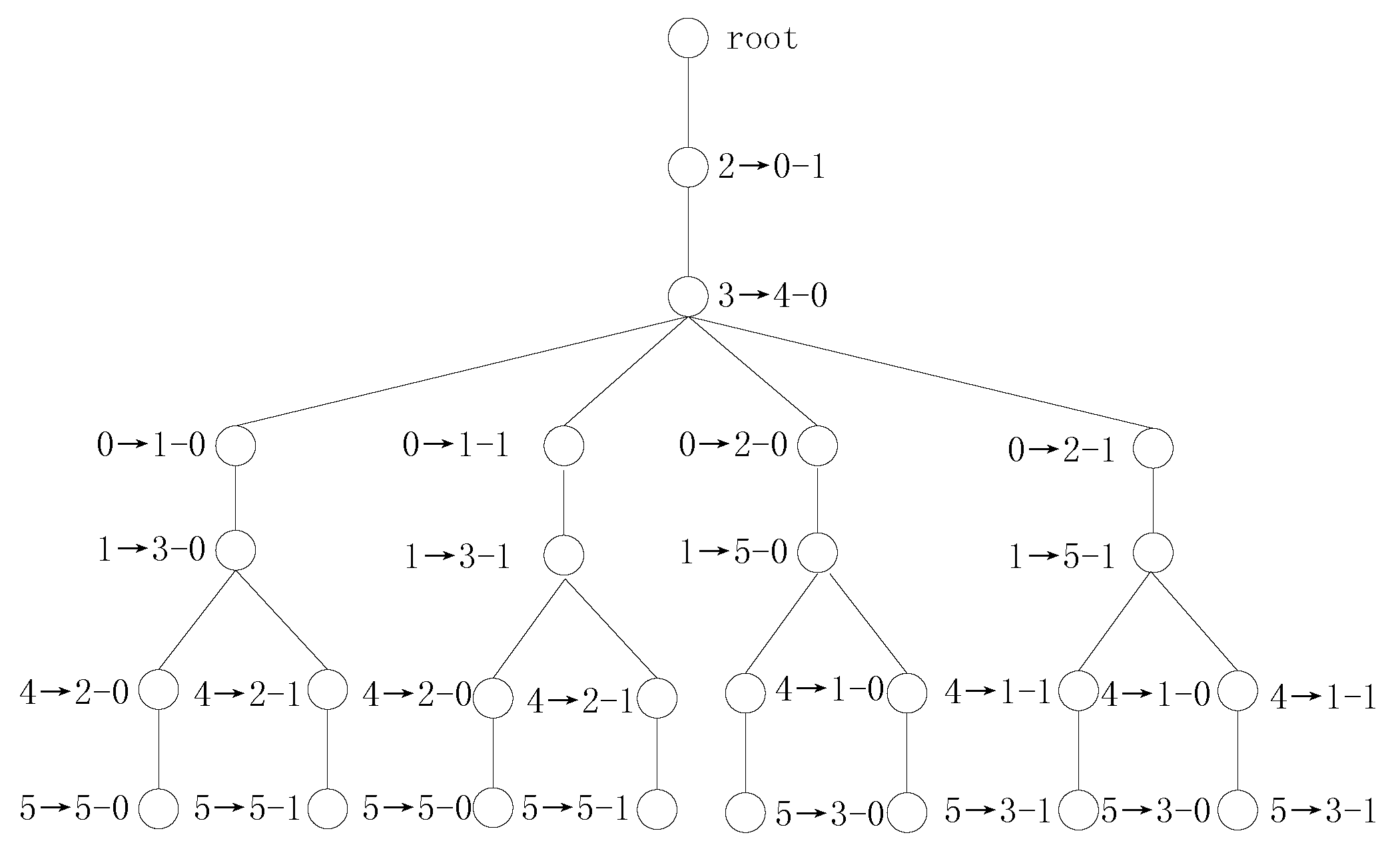
In Example 2, if we use the SS values to search the variable mappings, then there are one single symmetry-mapping set S 2 = { C 2 C 0 } and two multiple symmetry-mapping sets S 0 = { C 0 C 1 , C 0 C 2 } and S 4 = { C 4 C 1 , C 4 C 2 } , where S 0 = S 4 = 4 . Procedure 2 handles the single symmetry-mapping set S 2 , and the variable mappings x ¯ 2 x 0 and x 3 x 4 are added to t r a n s _ l i s t . s p _ f and s p _ g are updated to x ¯ 2 and x 0 . After the SS vectors are updated, the 1st signatures of the remaining variables of f and g are all ( 8 , 8 ) . Therefore, the remaining four variables still cannot be distinguished, and there are two multiple symmetry-mapping sets, S 0 and S 4 . The first symmetry-mapping set S 0 is selected to be handled. The transformation tree for Example 2 using SS vectors is shown in Figure 1.
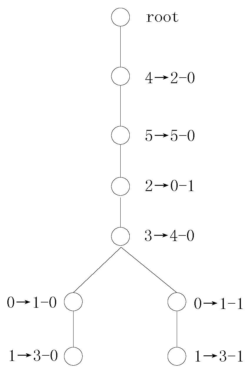
If we use the SDS values to search the variable mappings, then there are one independent-mapping set, one single symmetry-mapping set and one multiple symmetry-mapping set according to the first computed SDS vectors. Procedure 2 first adds the variable mappings x 4 x 2 and x 5 x 5 to the transformation tree. Then, the two variable mappings x ¯ 2 x 0 and x 3 x 4 of the symmetry mapping C 2 C 0 are added to the transformation tree. The catch is that the independent variable is not a splitting variable because the decomposition results obtained via Shannon expansion with the independent variable are unchanged. Thus, the decomposition expressions s p _ f and s p _ g are updated to x ¯ 2 and x 0 . UPDATE() is called to compute new SDS vectors, and the SDS vectors are updated in accordance with s p _ f and s p _ g .
In this way, Procedure 2 determines 4 variable mappings, namely, x 4 x 2 , x 5 x 5 , x ¯ 2 x 0 and x 3 x 4 , after the first variable mapping search for example 2. In the next variable mapping search, there is one multiple symmetry-mapping set, S 0 = { { x 0 x 1 , x 1 x 3 } , { x 0 x ¯ 1 , x 1 x ¯ 3 } } . The transformation tree for Example 2 using SDS vectors is shown in Figure 2.
From Example 2, we can see that the number of candidate transformations decreases from 8 to 2. The use of Boolean difference signatures helps to distinguish symmetry classes C 1 and C 5 , and we need to consider only the positive phase for independent variables. Thus, Boolean difference signatures are very beneficial for distinguishing variables.
In cell library binding, a benchmark Boolean circuit is found to realize another NPN equivalent Boolean function. Example 3 demonstrates the process of NPN equivalent matching by SS and SDS vectors respectively, and illustrates the validity of the SDS vectors proposed in this paper.
Example 3.
Consider two 6-input Boolean functions f ( X ) and g ( X ) :
f ( X ) = x 0 x 1 ( x 3 x 5 + x 4 x 5 ) + x 0 x ¯ 1 ( x 4 x ¯ 5 + x 2 x 3 x ¯ 4 x ¯ 5 ) + x 1 x ¯ 3 x ¯ 4 x ¯ 5 + x 1 x ¯ 2 x ¯ 4 x ¯ 5 + x ¯ 0 x ¯ 1 ( x ¯ 4 x 5 + x 2 x ¯ 3 x 4 x 5 ) + x ¯ 1 x ¯ 3 x ¯ 4 x 5 + x ¯ 0 x 1 ( x ¯ 2 x 3 x 4 + x 2 x ¯ 3 x 4 + x 3 x 4 x 5 + x 2 x ¯ 4 x ¯ 5 + x ¯ 2 x 4 x ¯ 5 ) + x ¯ 1 x 2 x 3 x 4 x ¯ 5 ,
g ( X ) = x ¯ 0 x 1 x 2 x ¯ 3 + x 0 x 1 x ¯ 2 x ¯ 3 + x ¯ 0 x ¯ 1 x ¯ 2 x 3 + x ¯ 0 x 1 x 2 x 5 + x ¯ 0 x 1 x 3 x 4 x ¯ 5 + x 0 x ¯ 1 x 2 x ¯ 5 + x 0 x 1 x ¯ 2 x 5 + x ¯ 0 x ¯ 1 x ¯ 2 x ¯ 3 x ¯ 4 + x ¯ 0 x ¯ 1 x 2 x ¯ 3 x 5 + x ¯ 0 x ¯ 1 x 2 x 4 x 5 + x ¯ 0 x ¯ 1 x ¯ 2 x 4 x ¯ 5 + x ¯ 0 x 1 x ¯ 2 x 3 x ¯ 4 x ¯ 5 + x 0 x 1 x 2 x 3 x ¯ 4 x ¯ 5 + x 0 x ¯ 1 x ¯ 2 x ¯ 3 x 4 x 5 .
The transformation detection process using SS vectors is as follows:
(1) Compute the SS vectors of f and g. The results are:
V f = { ( 16 , 16 , 1 , 1 , 1 ) , ( 19 , 13 , 1 , 1 , 0 ) , ( 16 , 16 , 1 , 1 , 1 ) , ( 16 , 16 , 1 , 1 , 1 ) , ( 16 , 16 , 1 , 1 , 1 ) , ( 16 , 16 , 1 , 1 , 1 ) } ,
V g = { ( 13 , 19 , 1 , 1 , 1 ) , ( 16 , 16 , 1 , 1 , 0 ) , ( 16 , 16 , 1 , 1 , 1 ) , ( 16 , 16 , 1 , 1 , 1 ) , ( 16 , 16 , 1 , 1 , 1 ) , ( 16 , 16 , 1 , 1 , 1 ) } .
From the above results, we can draw three conclusions: (1) these two SS vectors are the same; (2) the phases of the variable x 1 of f and the variable x 0 of g are determined; and (3) there is only one variable x 0 of g with the same SS values as those of the variable x 1 of f. Therefore, there is a single-mapping set { x 1 x ¯ 0 } . Concerning the splitting variables, the new splitting expressions are s p _ f = x 1 and s p _ g = x ¯ 0 .
(2) The algorithm enters the next iteration and computes the new SS vectors. The new SS vectors are:
V f = { ( 9 , 10 , 1 , 1 , 1 ) , ( 0 , 0 , 1 , 1 , 0 ) , ( 9 , 10 , 1 , 1 , 1 ) , ( 10 , 9 , 1 , 1 , 1 ) , ( 10 , 9 , 1 , 1 , 1 ) , ( 9 , 10 , 1 , 1 , 1 ) } ,
V g = { ( 0 , 0 , 1 , 1 , 1 ) , ( 9 , 10 , 1 , 1 , 0 ) , ( 10 , 9 , 1 , 1 , 1 ) , ( 10 , 9 , 1 , 1 , 1 ) , ( 10 , 9 , 1 , 1 , 1 ) , ( 10 , 9 , 1 , 1 , 1 ) } .
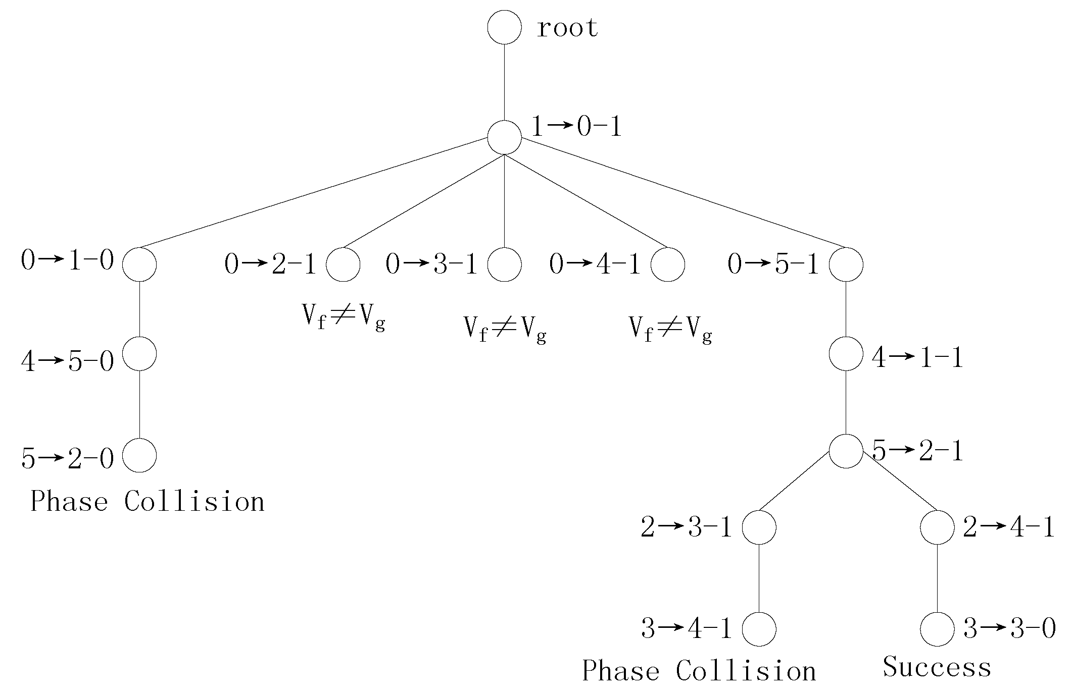
The results show the following: (1) the two new SS vectors are the same; (2) the phases of all variables are determined; and (3) the next variable-mapping set to be handled is χ 0 = { x ¯ 0 x ¯ 1 , x ¯ 0 x 2 , x ¯ 0 x 3 , x ¯ 0 x 4 , x ¯ 0 x 5 } . Procedure 2 adds 5 nodes to the second layer of the transformation tree. Procedure 2 handles the first variable mapping in the order of the variable mappings in the set and updates s p _ f = x 1 x ¯ 0 and s p _ g = x 0 x ¯ 1 .
In the subsequent variable mapping search, the x ¯ 0 x ¯ 1 branch is pruned by a phase collision. The x ¯ 0 x 2 , x ¯ 0 x 3 and x ¯ 0 x 4 branches are pruned by having different SS vectors.
(3) Then, Procedure 2 handles the variable mapping x ¯ 0 x 5 and detects a candidate transformation T = { x 1 x ¯ 0 , x ¯ 0 x 5 , x 4 x ¯ 1 , x ¯ 5 x 2 , x ¯ 2 x 4 , x ¯ 3 x ¯ 3 } . After verification, this transformation is found to satisfy f ( T X ) = g ( X ) . Therefore, f is NPN-equivalent to g.
The transformation tree for Example 3 using SS vectors is shown in Figure 3.
Figure 3 shows that this transformation tree for Example 3 has 6 branches and that the two Boolean functions are decomposed 4 times. Let us examine the detection process using SDS vectors.
(1) The SDS vectors of f and g are as follows:
V f = { ( 16 , 16 , 1 , 1 , 3 , 28 ) , ( 19 , 13 , 1 , 1 , 0 , 64 ) , ( 16 , 16 , 1 , 1 , 5 , 12 ) , ( 16 , 16 , 1 , 1 , 4 , 20 ) , ( 16 , 16 , 1 , 1 , 2 , 36 ) , ( 16 , 16 , 1 , 1 , 1 , 52 ) } ,
V g = { ( 13 , 19 , 1 , 1 , 0 , 64 ) , ( 16 , 16 , 1 , 1 , 2 , 36 ) , ( 16 , 16 , 1 , 1 , 1 , 52 ) , ( 16 , 16 , 1 , 1 , 4 , 20 ) , ( 16 , 16 , 1 , 1 , 5 , 12 ) , ( 16 , 16 , 1 , 1 , 3 , 28 ) } .
From these results, we can draw the following conclusions: (1) these two SDS vectors are the same; (2) the phases of the variable x 1 of f and the variable x 0 of g are determined,; and (3) there is one single-mapping set { x 1 x ¯ 0 } to be used in the search. In Procedure 2, the splitting variables x 1 and x ¯ 0 are used to decompose f and g, respectively.
(2) The new SDS vectors are as follows:
V f = { ( 9 , 10 , 1 , 1 , 3 , 14 ) , ( 0 , 0 , 1 , 1 , 0 , 64 ) , ( 9 , 10 , 1 , 1 , 5 , 6 ) , ( 10 , 9 , 1 , 1 , 4 , 10 ) , ( 10 , 9 , 1 , 1 , 2 , 18 ) , ( 9 , 10 , 1 , 1 , 1 , 26 ) } ,
V g = { ( 0 , 0 , 1 , 1 , 0 , 64 ) , ( 9 , 10 , 1 , 1 , 2 , 18 ) , ( 10 , 9 , 1 , 1 , 1 , 26 ) , ( 10 , 9 , 1 , 1 , 4 , 10 ) , ( 10 , 9 , 1 , 1 , 5 , 6 ) , ( 10 , 9 , 1 , 1 , 3 , 14 ) } .
From these two new SDS vectors, the following can be seen: (1) the phases of all variables are determined; and (2) all unidentified variables can be identified from their Boolean differences. A candidate transformation T = { x 1 x ¯ 0 , x ¯ 0 x 5 , x ¯ 2 x 4 , x 3 x 3 , x 4 x ¯ 1 , x ¯ 5 x 2 } is generated, and this T is verified to be correct.
When SDS vectors are used to perform Boolean matching, the transformation tree for Example 3 contains only one candidate transformation. In the transformation detection process, the search space comprises all branches of the transformation tree, including unabridged and abridged branches. The unabridged branches are the candidate transformations, and the abridged branches are the pruned transformations. When the transformation tree possesses fewer branches, the algorithm considers a smaller search space. The purpose of decomposing the Boolean functions is to update the SDS vectors to search the new variable mappings. When the algorithm requires fewer decompositions, more variables are identified in each iteration. These three indicators can be used to measure how much of the search space our algorithm searches.
In the best case, the variable mapping set of every variable is a single-mapping set, and there is only one candidate transformation. In this case, the spatial complexity is O ( 1 ) , and the time complexity is O ( n 2 ) . In the worst case, there are no symmetric variables, every variable has the same SDS value, and the phases of all variables cannot be determined in each SDS update. There are 2 n + 1 n ! candidate transformations that need to be verified. The spatial complexity is O ( 2 n n ! ) , and the time complexity is O ( n 3 ) .

5. Experimental Results

To demonstrate the effectiveness of the proposed method, we re-implemented the algorithm of [6] and tested the algorithm presented in this paper, the algorithm of [5] and the algorithm of [6] on both a randomly generated circuit set and an MCNC benchmark circuit set. In the random circuit set, there were 1200 circuits in each input circuit set. Every circuit in the random circuit set contained at least two candidate transformations. In the test, we recorded the three indicators concerning the search space and the run time. The proposed algorithm was implemented in C with buddy package. The following experimental results were obtained in a hardware environment with a 3.3-GHz Intel Xeon processor and 4 GB of memory.
In the following tables, the first column shows the number of input variables (#I), and the following four columns show the experimental results for our algorithm. The next four columns show the corresponding experimental results of [5], and the last column shows the average run time of the algorithm of [6].
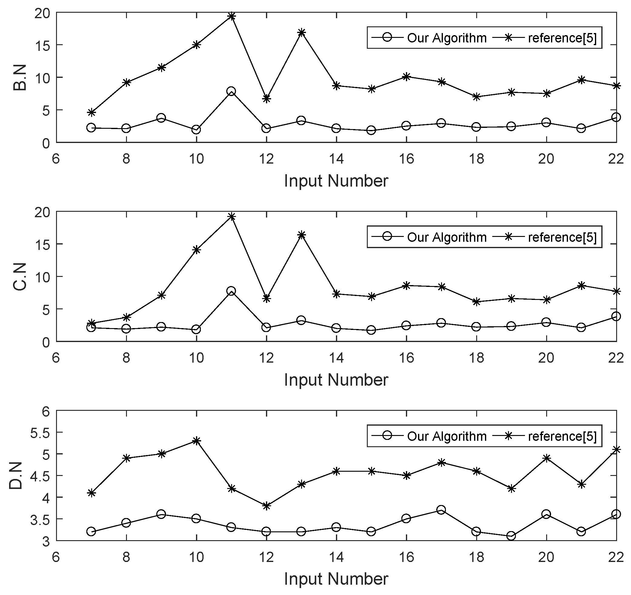
Table 1 and Table 2 show the average number of branches (#B.N.), the average number of candidate transformations (#C.N.), the average number of decompositions (#D.N.) and the average run time (#R.T.) of our algorithm and of the algorithm of [5] on the random circuit set and on the MCNC benchmark circuit set, respectively.
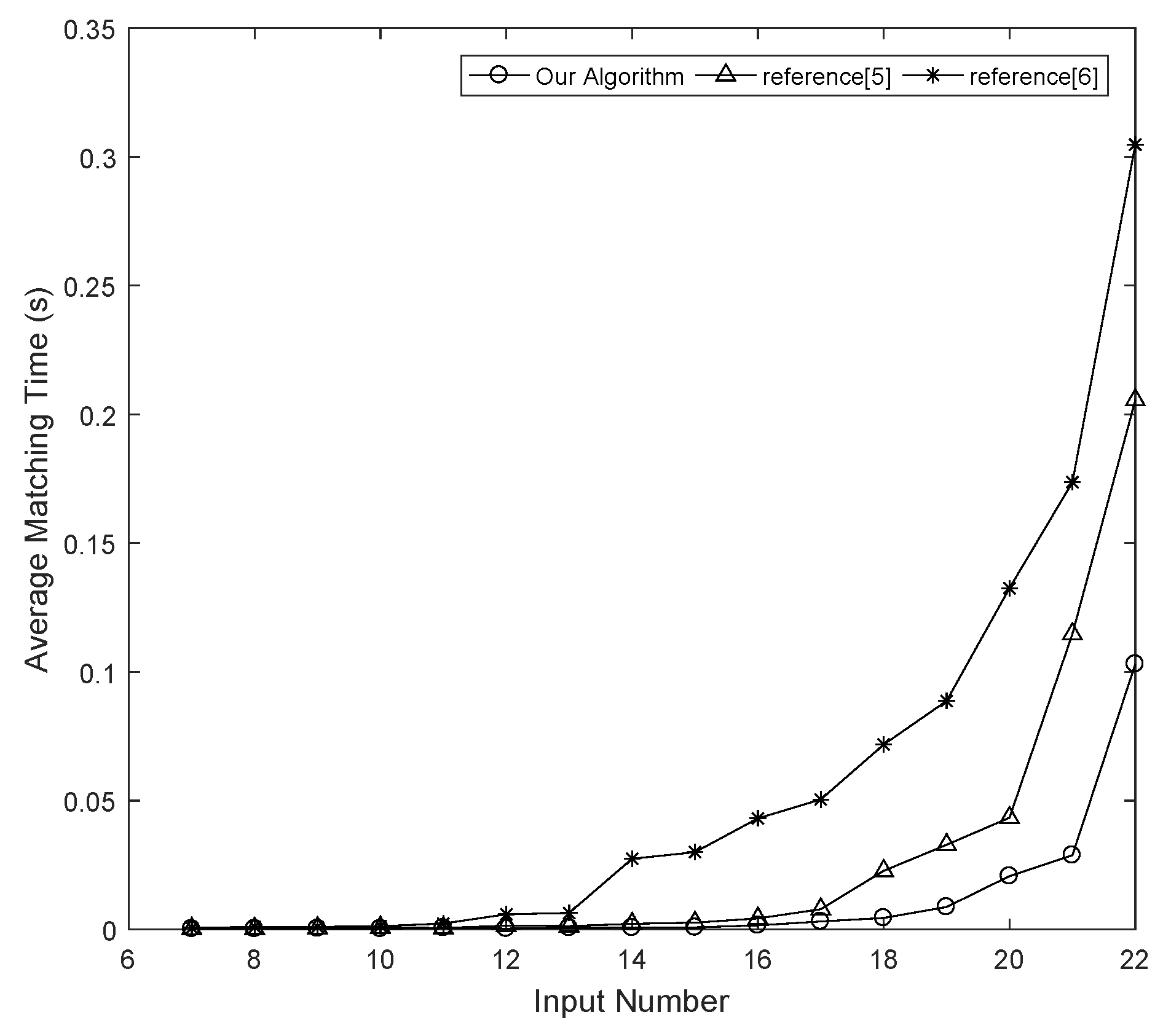
From Table 1, we can see that the run time of our algorithm is improved by 54% relative to that of [5] and by 84% relative to that of [6]. From the comparison of the three indicators for the search space, we can see that the number of branches in the transformation tree is reduced by 70%, the number of candidate transformations is reduced by 65%, and the number of decompositions is reduced by 27%. Because the Boolean difference facilitates the identification of the variables, the proposed algorithm reduces the search space and speeds up the matching process. Figure 4 presents the diagram of the search space comparison results for our algorithm and that of reference [5] tested on the random circuit set.
Figure 5 presents the diagram of the speed comparison results for our algorithm, that of reference [6] and that of reference [5] tested on the random circuit set.
Table 2 shows the experimental results obtained during testing on the MCNC benchmark circuit set.
Table 2 shows that with the proposed algorithm, the values of the three indicators for the search space are decreased, and the run time is also slightly reduced. When there are 22 inputs, however, the average run time of our algorithm is higher than that of [5]. This is because the variables of this group circuit are easy to identify and because the search space of our algorithm is almost the same as that of [5]. In this case, our algorithm spends additional time in computing the Boolean differences compared with the algorithm of [5].
From Table 1 and Table 2, we can see that the matching speed on the MCNC benchmark circuits is slower than that on random circuits, although the search space for the MCNC benchmark circuits is less than that for the random circuits. In this paper, we use BDDs to represent Boolean functions. The BDD structure of a Boolean function is closely related to the speed of operations on the BDD. Because the BDD operation speed on the MCNC benchmark circuits is slower than that on the random circuits, the matching speed on the MCNC benchmark circuits is also slower than that on the random circuits.

6. Conclusions

The major contribution of this paper is the raise of SDS vector. The paper demonstrates how SDS vectors can be used to effectively search variable mappings and reduce the search space. The algorithm of this paper take advantage of cofactor, symmetry and Boolean different when search the variable mappings between two Boolean functions. Therefore, the search space and match speed of ours algorithm is better than the competitors. Compared with the algorithm of [5], the search space is cut in 48%, and the run time is reduced by 42% and 80% compared with [5,6], respectively. The experimental results prove that the algorithm proposed in this paper is more effective than competing algorithms on general circuits. In future work, we will extend our algorithm to multiple-output Boolean matching and Boolean matching with don’t care sets.

Author Contributions

J.Z. proposed and implemented the algorithm. G.Y. was the research advisor and provided suggestions. W.N.N.H. provided guidance for this paper and contributed to the revisions and gave advice on optimization issues. J.W. and Y.Z. completed the generation of data and test.

Funding

This research was funded by the National Natural Science Foundation of China Grant (Nos. 61572109, 11371003 and 61751110), the Special Fund for Bagui Scholars of Guangxi (Grant No. 113000200230010), Network and Data Security Key Laboratory of Sichuan Province Open Project (NDSMS201603).

Acknowledgments

We would like to thank the above funds for their technical and financial support.

Conflicts of Interest

The authors declare no conflict of interest.

References

  1. Slepian, D. On the number of symmetry types of Boolean functions of n variables. Can. J. Math. 1955, 2, 185–193. [Google Scholar] [CrossRef]
  2. Zhang, J.; Yang, G.; Hung, W.N.N.; Liu, T.; Song, X.; Perkowski, M.A. A group algebraic approach to NPN classification of Boolean functions. Theory Comput. Syst. 2018. [Google Scholar] [CrossRef]
  3. Zhang, Y.; Yang, G.; Hung, W.N.N.; Zhang, J. Computing affine equivalence classes of Boolean functions by group isomorphism. IEEE Trans. Comput. 2016, 12, 3606–3616. [Google Scholar] [CrossRef]
  4. Lai, Y.-T.; Sastry, S.; Pedram, M. Boolean matching using binary decision diagrams with applications to logic synthesis and verification. In Proceedings of the 1992 IEEE International Conference on Computer Design: VLSI in Computers and Processors, Cambridge, MA, USA, 11–14 October 1992. [Google Scholar] [CrossRef]
  5. Zhang, J.; Yang, G.; Hung, W.N.N.; Zhang, Y.; Wu, J. An efficient NPN Boolean matching algorithm based on structural signature and Shannon expansion. Cluster Comput. 2018, 6, 1–16. [Google Scholar] [CrossRef]
  6. Adbollahi, A.; Pedram, M. Symmetry detection and Boolean matching utilizing a signature-based canonical form of Boolean functions. IEEE Trans. Comput.-Aided Des. Integr. Circuits Syst. 2008, 6, 1128–1137. [Google Scholar] [CrossRef]
  7. Lee, S.Y.; Lee, N.Z.; Jiang, J.H.R. Canonicalization of threshold logic representation and its applications. In Proceedings of the International Conference on Computer-Aided Design, San Diego, CA, USA, 5–8 November 2018; p. 85. [Google Scholar]
  8. Asghar, A.; Iqbal, M.M.; Ahmed, W.; Ali, M.; Parvez, H.; Rashid, M. Logic algebra for exploiting shared SRAM-table based FPGAs for large LUT inputs. In Proceedings of the Electrical Engineering and Computing Technologies, Karachi, Pakistan, 15–16 November 2017; pp. 1–4. [Google Scholar] [CrossRef]
  9. Soeken, M.; Mishchenko, A.; Petkovska, A.; Sterin, B.; Ienne, P.; Brayton, R.K.; De Micheli, G. Heuristic NPN classification for large functions using AIGs and LEXSAT. In Proceedings of the International Conference on Theory and Applications of Satisfiability Testing, Bordeaux, France, 5–8 July 2016; pp. 212–227. [Google Scholar]
  10. Huang, Z.; Wang, L.; Nasikovskiy, Y.; Mishchenko, A. Fast Boolean matching based on NPN classification. In Proceedings of the International Conference on Field-Programmable Technology, Kyoto, Japan, 9–11 December 2013; pp. 310–313. [Google Scholar] [CrossRef]
  11. Petkovska, A.; Soeken, M.; Micheli, G.D.; Ienne, P.; Mishchenko, A. Fast hierarchical NPN classification. In Proceedings of the International Conference on Field Programmable Logic and Applications, Lausanne, Switzerland, 29 August–2 September 2016; pp. 1–4. [Google Scholar] [CrossRef]
  12. Agosta, G.; Bruschi, F.; Pelosi, G.; Sciuto, D. A transform-parametric approach to Boolean matching. IEEE Trans. Comput.-Aided Des. Integr. Circuits Syst. 2009, 6, 805–817. [Google Scholar] [CrossRef]
  13. Chen, K.C.; Yang, C.Y. Boolean matching algorithms. In Proceedings of the International Symposium on VLSI Technology, Systems, and Applications, Taipei, Taiwan, 12–14 May 1993; pp. 44–48. [Google Scholar]
  14. Kapoor, B. Improved technology mapping using a new approach to Boolean matching. In Proceedings of the European Design and Test Conference, Paris, France, 6–9 March 1995; pp. 86–90. [Google Scholar] [CrossRef] [Green Version]
  15. Vos, A.D.; Baerdemacker, S.D. Symmetry groups for the decomposition of reversible computers, quantum computers, and computers in between. Symmetry 2011, 2, 305–324. [Google Scholar] [CrossRef]
  16. Katebi, H.; Igor, I.L. Large-scale Boolean matching. In Proceedings of the Conference on Design, Automation and Test in Europe, Dresden, Germany, 8–12 March 2010; pp. 771–776. [Google Scholar] [CrossRef]
  17. Matsunaga, Y. Accelerating SAT-based Boolean matching for heterogeneous FPGAs using one-hot encoding and CEGAR technique. In Proceedings of the Design Automation Conference of 20th Asia and South Pacifics, Chiba, Japan, 19–22 January 2015; pp. 255–260. [Google Scholar] [CrossRef]
  18. Ghaderi, Z.; Bagherzadeh, N.; Albaqsami, A. STABLE: Stress-Aware Boolean Matching to Mitigate BTI-Induced SNM Reduction in SRAM-Based FPGAs. IEEE Trans. Comput. 2018, 99, 1. [Google Scholar] [CrossRef]
  19. Cong, J.; Minkovich, K. Improved SAT-based Boolean matching using implicants for LUT-based FPGAs. In Proceedings of the ACM/sigda International Symposium on Field Programmable Gate Arrays, Monterey, CA, USA, 18–20 February 2007; pp. 139–147. [Google Scholar]
  20. Wang, K.H.; Chan, C.M.; Liu, J.C. Simulation and SAT-based Boolean matching for large Boolean networks. In Proceedings of the Design Automation Conference, San Francisco, CA, USA, 26–31 July 2009; pp. 396–401. [Google Scholar]
  21. Moore, J.; Fazel, K.; Thornton, M.A.; Miller, D.M. Boolean function matching using Walsh Spectral decision diagrams. In Proceedings of the Design, Applications, Integration and Software, Richardson, TX, USA, 29–30 October 2006; pp. 127–130. [Google Scholar] [CrossRef]
  22. Thornton, M.A.; Drechsler, R.; Gunther, W. Logic circuit equivalence checking using Haar Spectral coefficients and partial BDDs. VLSI Des. 2014, 1, 53–64. [Google Scholar] [CrossRef]
  23. Zhang, J.S.; Chrzanowska-Jeske, M.; Mishchenko, A.; Burch, J.R. Linear cofactor relationships in Boolean functions. IEEE Trans. Comput.-Aided Des. Integr. Circuits Syst. 2006, 6, 1011–1023. [Google Scholar] [CrossRef]
Figure 1. The transformation search tree for example 2 using SS vectors.
Symmetry 11 00027 g001
Figure 2. The transformation search tree for example 2 using SDS vectors.
Symmetry 11 00027 g002
Figure 3. The transformation search tree for example 3 using SS vectorss.
Symmetry 11 00027 g003
Figure 4. The search space comparison results for testing on random circuits.
Symmetry 11 00027 g004
Figure 5. The matching speed comparison results for testing on random circuits.
Symmetry 11 00027 g005
Table 1. Boolean matching results on random circuits.
#I#B.N.#C.N.#D.N.#R.T.#B.N. of [5]#C.N. of [5]#D.N. of [5]#R.T. of [5]#R.T. of [6]
72.22.13.20.000244.62.84.10.000240.00067
82.11.93.40.000229.23.74.90.000300.00091
93.72.23.60.0003411.57.15.00.000470.00099
101.91.83.50.0002715.014.15.30.000740.00123
117.87.73.30.0005919.419.24.20.000530.00228
122.12.13.20.000326.76.63.80.001460.00585
133.33.23.20.0006116.916.44.30.001270.00638
142.12.03.30.000638.77.34.60.002170.02743
151.81.73.20.000798.26.94.60.002620.02998
162.52.43.50.0015510.18.64.50.004260.04310
172.92.83.70.003089.38.44.80.007840.05044
182.32.23.20.004457.06.14.60.022740.07177
192.42.33.10.008707.76.64.20.032850.08870
203.02.93.60.020697.56.44.90.043370.13250
212.12.13.20.028799.68.64.30.114710.17362
223.83.83.60.103018.77.75.10.205540.30469
Table 2. Boolean matching results on MCNC benchmark circuitsd.
#I#B.N.#C.N.#D.N.#R.T.#B.N. of [5]#C.N. of [5]#D.N. of [5]#R.T. of [5]#R.T. of [6]
71.01.01.50.000141.31.01.80.000120.00121
81.11.13.20.000421.21.23.50.000350.00146
91.21.21.80.000341.61.52.40.000510.00186
101.11.11.30.000603.41.51.50.000630.00193
111.01.01.30.000741.41.42.60.000780.00243
121.01.01.30.000801.31.21.70.000910.00255
131.11.02.50.004671.31.13.80.004470.00535
141.11.11.40.004011.21.12.00.003680.01245
151.41.32.00.005691.71.53.10.004750.04077
161.21.21.90.013462.01.63.20.001510.04849
171.11.11.50.105021.21.22.20.115180.31644
181.11.01.50.109441.51.52.50.233940.64273
191.81.82.60.807475.55.34.40.891231.62971
201.31.32.11.003092.92.82.71.281562.13035
211.31.31.53.730721.71.52.73.7138210.2122
221.61.61.76.501302.82.73.16.2436811.2760