Degree Reduction of S-λ Curves Using a Genetic Simulated Annealing Algorithm

Abstract

The S-λ Curves have become an important research subject in computer aided geometric design (CAGD), which owes to its good geometric properties (such as affine invariance, symmetry, and locality). This paper presents a new method to approximate an S-λ curve of degree n by using an S-λ curve of degree n-1. We transform this degree reduction problem into the function optimization problem first, and then using a new genetic simulated annealing algorithm to determine the global optimal solution of the optimization problem. The method can be used to approximate S-λ curves with fixed or unconstrained endpoints. Examples are given to verify the effectiveness of the presented algorithm; and these numeric examples show that the algorithm is not only easy to implement, but also offers high precision, which makes it valuable in practical applications.

1. Introduction

Many methods used in Computer Aided Geometric Design (CAGD) are closely associated with probability distributions, particularly discrete distributions (Johnson et al., 2005 [1]). For example, the Bernstein basis functions used in Bézier curves are related to the binomial distribution, the B-spline basis functions used in B-spline curves are connected with some stochastic processes (Dahmen et al., 1986 [2], Goldman et al., 2000 [3], Hu et al., 2018 [4,5,6,7]), the Poisson basis functions introduced by Goldman and Morin (2000) were developed from the Poisson distribution, and the Bernstein basis functions of negative degree presented by Goldman (1999) are taken from the negative binomial distribution [8]. These basis functions and other basis functions generated from discrete distributions, are important in the approximation process based on approximation theory (Hahn 1980 [9], Khan 1980 [10], Omey 1996 [11], De La Cal J. 1993 [12], Zeng 2005 [13], Zeng and Cheng 2001 [14]). On the basis of these points, Fan and Zeng [15] have explored a novel class of discrete distributions known as S-λ distributions. The curves generated from S-λ distributions are called S-λ curves, which include Bézier curves, Poisson curves, rational Bézier curves, and many others.

Degree reduction of curves and surfaces has important practical significance because the approximation of curves and surfaces by other curves and surfaces of different degree is crucial to data conversion, transmission and compression (Watkins & Worsey 1988 [16], Lutterkort 1999 [17]). However, the efficiency and stability of the existing degree reduction algorithms still have much room for improvement. Two classes of methods for this purpose have been studied extensively. The first class is geometric method based on control points, which is an inverse process of degree elevation and has been used to determine the control points of degree-reduced curves (Ren et al., 2007 [18]). This method utilizes the geometric properties of the Bézier curve itself and some mathematical theories including generalized inverse matrix method, the best uniform approximation and the least squares approximation theory to achieve the degree reduction of Bézier curve (Cai et al., 2010 [19], Ahn et al., 2004 [20]). Moreover, some other scholars realize degree reduction of Bézier curves and surfaces by perturbing control vertices and using constrained optimization method (Lu et al., 2009 [21], Lu & Wang 2006 [22], Delgado et al., 2007 [23], Ait-Haddou & Bartoň 2016 [24]). The second class is algebraic method based on basis function transformation. In one example that utilized this approach, degree reduction was achieved by constraining Legendre polynomials (Liang et al., 2006 [25]). Similarly, based on Chebyshev polynomials (Rababah et al., 2006 [26], Lu et al., 2008 [27]) or Jacobi polynomials (Xu et al., 2008 [28]), the degree reduction of Bézier curves can be come true. A final interesting group of studies have focused on the problem of the approximate degree reduction of C-Bézier curves (Wang 2009 [29], Qin et al., 2013 [30]). Here we present a new method for the degree reduction of S-λ curves approximately based on a genetic simulated annealing algorithm.

The outline of this paper is as follows. The definition of S-λ curves is described in Section 2. In Section 3, we investigate the degree reduction of S-λ curves using an intelligent algorithm. Finally, a short conclusion is given in Section 4.

2. Definition of S-λ Curves

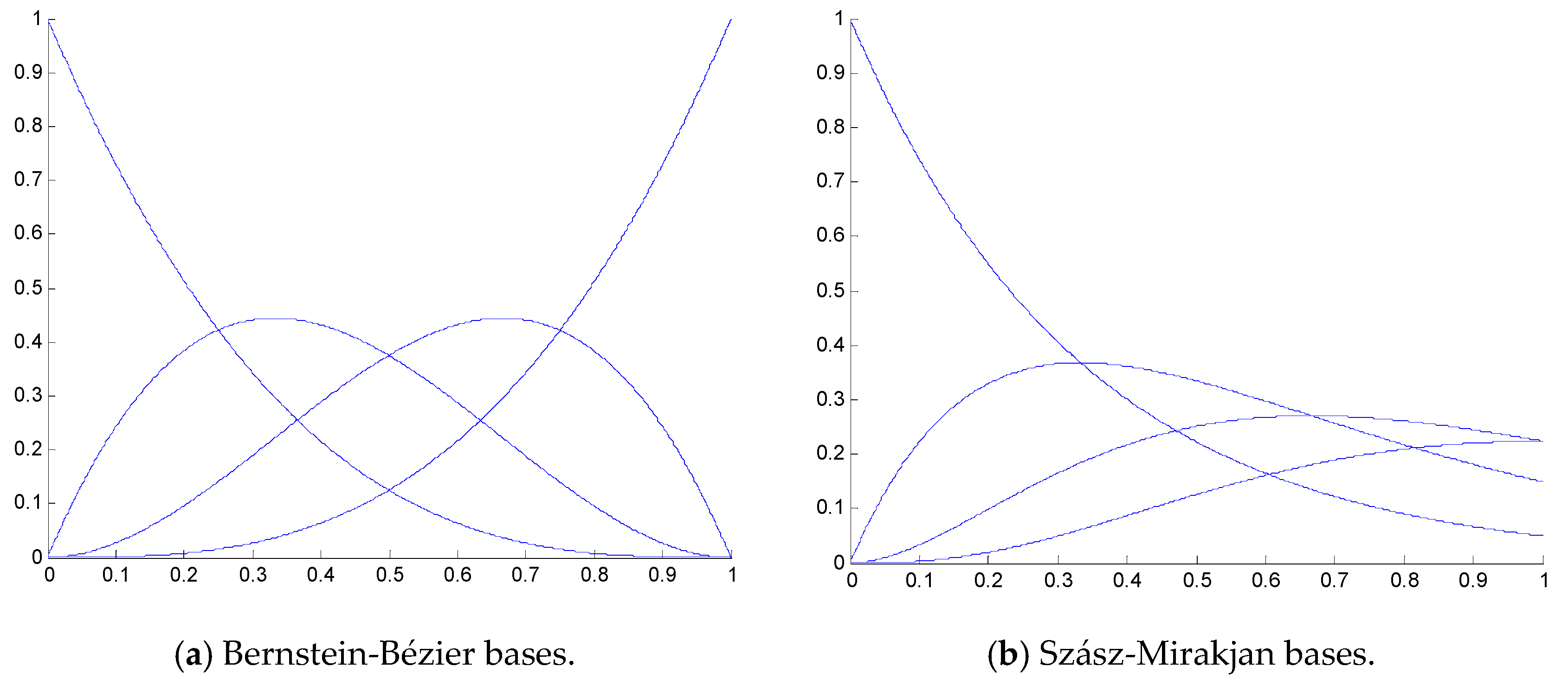
2.1. S-λ Distributions and Basis Functions

Let ${\left\{A_j\right\}}_{j=0}^m$ be a given sequence of positive numbers, where m may be equal to $+\infty$. The generating function (gf) of the sequence is $S(x)={\displaystyle \sum {}_{j=0}^m{A}_j{x}^j}$, which satisfies $S(0)=1$. Furthermore, suppose the convergence radius of $S(x)$ is $R$ and, let $\lambda (x)$ be a strictly continuous monotone increasing function satisfying $\lambda (0)=0$ and mapping $[0,R_1)$ onto $[0,R)$, where R and R₁ may be equal to $+\infty$. $\lambda (x)$ is called the transformation factor (tf). For $x\in [0,R_1)$, setting $P_{1,j}(x)=\frac{A_j{[\lambda (x)]}^j}{S[\lambda (x)]}$, and then $P_{1,j}(x)\in C[0,R_1)$ and ${\displaystyle \sum {}_{j=0}^m{P}_{1,j}(x)=1}$. Now we give the following definition (Fan and Zeng 2012 [15]).

Definition 1.

Let$\xi$be an integer random variable satisfying:

$$P(\xi =j)=P_{1,j}(x)=\frac{A_j{[\lambda (x)]}^j}{S[\lambda (x)]}(j=0,1,\dots ,m).$$

(1)

${\left\{A_j^{(n)}\right\}}_{j=0}^{mn}$is an n-convolution of${\left\{A_j\right\}}_{j=0}^m$with the generating function:

$$S_n(x)={[S(x)]}^n={\displaystyle \sum _{j=0}^{mn}{A}_j^{(n)}{x}^j},x\in [0,R_1).$$

(2)

Let${\left\{{\xi }_i\right\}}_{i=1}^{\infty }$be a sequence of independent random variables with the same distribution as$\xi$. Set${\eta }_n={\displaystyle \sum {}_{i=1}^n{\xi }_i}$. Then by the convolution formula of probability, we can obtain:

$$P({\eta }_n=j)=\frac{A_j^{(n)}{[\lambda (x)]}^j}{S_n[\lambda (x)]}(j=0,1,\dots ,mn).$$

(3)

We call the probability distributions (3) S-λ distributions. If we write:

$$P_{n,j}(x)=\frac{A_j^{(n)}{[\lambda (x)]}^j}{S_n[\lambda (x)]},(x\in [0,R_1),j=0,1,\dots ,mn),$$

(4)

and then$P_{n,j}(x)$are called the S-λ basis functions corresponding to S-λ distributions.

From Definition 1, two properties of $P_{n,j}(x)\ge 0$ and ${\sum }_{j=0}^{mn}{P}_{n,j}(x)=1$ are true obviously. According to Definition 1, we can construct different S-λ distributions by selecting appropriate generating functions $S(x)={\displaystyle \sum {}_{j=0}^m{A}_j{x}^j}$ and transformation factors $\lambda (x),x\in [0,R_1)$. We give two interesting instances as follows.

Example 1.

Let$S(x)=1+x$and$\lambda (x)=\frac{x}{1-x}$, ($x\in [0,1)$); then${\left\{A_j\right\}}_{j=0}^1=\{1,1\}$. By convolving n-times we get:

$$A_j^{(n)}={\displaystyle \sum _{k=0}^j{A}_k^{(n-1)}{A}_{j-k}^{(1)}}=\left(\begin{array}{c}n\\ j\end{array}\right),j=0,1,\dots ,n.$$

(5)

By recombining the transformation factor and generating function, we have:

$$S_n[\lambda (x)]={[1+\lambda (x)]}^n={(1-x)}^{-n}.$$

Therefore, according to Definition 1 we obtain the classical Bernstein basis of degree n:

$$P_{n,j}(x)=\frac{A_j^{(n)}{[\lambda (x)]}^j}{S_n[\lambda (x)]}=\left(\begin{array}{c}n\\ j\end{array}\right)x^j{(1-x)}^{n-j},x\in [0,1),j=0,1,\dots ,n.$$

(6)

and the basis functions in (6) are shown in Figure 1a [15].

Example 2.

Letting$S(x)=e^x$and$\lambda (x)=x$,$x\in [0,+\infty )$, we can get$S_n[\lambda (x)]=e^{nx}$,$m=\infty$and${\left\{A_j\right\}}_{j=0}^{\infty }={\left\{\frac{1}{j!}\right\}}_{j=0}^{\infty }$. By taking n-times convolution operation of the infinite sequence${\left\{A_j\right\}}_{j=0}^{\infty }$, we have:

$$A_j^{(n)}=\frac{n^j}{j!}.$$

(7)

Thus, we can get the Poisson basis functions:

$$P_{1,j}(x)=\frac{A_j{[\lambda (x)]}^j}{S[\lambda (x)]}=\frac{e^{-x}{x}^j}{j!},$$

(8)

and the Szász-Mirakjan basis functions (see Figure 1b)

$$P_{n,j}(x)=\frac{A_j^{(n)}{[\lambda (x)]}^j}{S_n[\lambda (x)]}=\frac{e^{-nx}{(nx)}^j}{j!}.$$

(9)

2.2. S-λ Curves

Definition 2.

Let$\mathrm{V}={\left\{V_j\right\}}_{j=0}^{mn}$be a given set of the control points,$V_j\in R^3(j=0,1,\dots ,mn)$, then an S-λ curve of degree n can be defined as follows [15]:

$$C(t)={\displaystyle \sum _{j=0}^{mn}}{P}_{n,j}(t)V_j,t\in [0,R_1),$$

(10)

where$n\ge 1$, the number of m may be finite or infinite. However, since this paper focuses on practical applications, only the case of finite m is considered here. Some illustrative S-λ curves are discussed below.

Example 3.

Suppose that${\left\{V_j\right\}}_{j=0}^4=\left\{(0,0);(-5,6);(5,12);(15,6);(10,0)\right\},$$S(t)={\displaystyle \sum _{j=1}^4}{A}_j{t}^j$and$\lambda (t)=\frac{t}{1-t}$where$m=4,n=1$and$R_1=1$. The corresponding S-λ curve is$C(t)={\displaystyle \sum _{j=0}^4}{P}_{1,j}(t)V_j$. Figure 2 shows the curves C(t) with different generating functions S(t). From Figure 2, we can see clearly that if the j-th coefficient A_j of the generating functions is even bigger, then the corresponding S-λ curve is even closer to the control point V_j [15].

3. Degree Reduction of S-λ Curves Using an Intelligent Algorithm

3.1. The Degree Reduction Problem

Degree reduction for S-λ curves of degree n means finding a collection of control points on the S-λ curve of degree n-1, that is:

$$\overline{C}(t)={\displaystyle \sum _{j=0}^{m(n-1)}}{P}_{n-1,j}(t){\overline{V}}_j,t\in [0,R_1),$$

(11)

and the initial curve $C(t)$ and the degree-reduced curve $\overline{C}(t)$ satisfy the following condition:

$$\underset{0\le t<R_1}{\max }d[C(t),\overline{C}(t)]=\underset{0\le t<R_1}{\max }{\Vert C(t)-\overline{C}(t)\Vert }_2\to \min ,$$

(12)

where the operator $d[\cdot ,\cdot ]$ represents the Euclidean distance of the vector.

This problem can be translated into the following constrained optimization problem:

$$\begin{array}{c}f(\mathrm{V},\overline{\mathrm{V}},t)=\min \underset{0\le t<R_1}{\max }d(C(t),\overline{C}(t))=\min \underset{0\le t<R_1}{\max }{\Vert C(t)-\overline{C}(t)\Vert }_2\\ \mathrm{s}.\mathrm{t}.V_j,\overline{V_j}\in {\mathrm{R}}^3,t\in [0,R_1),\end{array}$$

(13)

where $\mathrm{V}={\left\{V_j\right\}}_{j=0}^{mn}$ and $\overline{\mathrm{V}}={\left\{{\overline{V}}_j\right\}}_{j=0}^{m(n-1)}$ represent the control point vectors of the initial S-λ curve and the degree-reduced S-λ curve, respectively.

3.2. Basic Principles of the Degree Reduction for S-λ Curve

3.2.1. Elementary Algorithms

The simulated annealing algorithm is inspired by the annealing of hot physical objects, proposed by Metropolis et al. in 1953. It is an efficient way for finding a global optimal solution of a given problem. The process begins by generating an initial solution, we take it as the current solution; a nonlocal optimal solution in the vicinity of the current solution is then chosen and the algorithm decides whether to move to the new solution or not using a probability p. This algorithm not only has no prematurity, but also avoid trapping the optimal solution into local optimization. The temperature is gradually reduced (similar to the annealing of a real object), which makes the activity of the system decrease until it stabilizes in the vicinity of the global minimum with a probability of 1.

The concepts of genetic algorithms are based on Darwin’s theory of biological evolution and Mendelian genetics [30,31,32,33]. They combine Darwin’s theory of survival of the fittest with random exchange theory to create a statistical model that is applicable to the evolution of natural systems and, more generally, as a universal adaptive search method for solving optimization problems. In a genetic algorithm, the parameters of the problem need to be solved are coded as chromosomes, and then exchanging their information through iterative selection, crossover and mutation, until the ‘ideal’ chromosomes are obtained. However, during initial iterations of the genetic algorithm, it is possible for some superior chromosomes to rapidly propagate throughout the population, this phenomenon is prematurity.

In this paper, we attempt to overcome the prematurity problem of genetic algorithms by combining them with complementary simulated annealing methods. In addition, we present a method for selecting a fitness function, which makes the algorithm more efficient and increases the convergence speed to global optimal solution.

3.2.2. Initialization of the Control Parameters and the Group

To use a genetic algorithm or simulated annealing method, we must define the values of several control parameters including the size of the population, the maximum number of evolutionary generations, the probability of crossover, the probability of mutation, the initial temperature, the cooling factor, and the final temperature. Generally, since the parameters of a problem cannot convert into the terms of a genetic algorithm directly, it is necessary to translate the feasible solutions of the problem into chromosomes or individuals within genetic space first. Various coding techniques can be used for this purpose containing binary coding, Greg coding, real-valued coding, and multi-level parameter coding. We adopt real-valued coding in this work because most real-valued optimization problems used this method do not require numerical conversion, which makes they can utilize genetic algorithms directly.

The populations of interest in this work are the feasible solutions of the control points for the degree-reduced S-λ curve. The first step in the initialization process is to generate a random number ${\alpha }_j\in [0,1],j=0,1,\dots ,m(n-1)$, and then applying the following equation to compute a set of control points in the interval $[V_{\min },V_{\max }]$.

$${\overline{V}}_j=V_{\min }+{\alpha }_j(V_{\max }-V_{\min }),j=0,1,\dots ,m(n-1),$$

(14)

where ${\overline{V}}_j$ represents a coordinate component of the control point vector ${\overline{V}}_j=({\overline{x}}_j,{\overline{y}}_j,{\overline{z}}_j)$ for the degree-reduced S-λ curve $\overline{C}(t)$; that is to say, ${\overline{V}}_j$ can be taken as the coordinate component ${\overline{x}}_j$, or ${\overline{y}}_j$, or ${\overline{z}}_j$. The symbol $V_{\min }$ and $V_{\max }$ is a coordinate component of the vector $V_{\min }=(x_{\min },y_{\min },z_{\min })$ and $V_{\max }=(x_{\max },y_{\max },z_{\max })$, respectively; the coordinate components of the vectors $V_{\min }$ and $V_{\max }$ are calculated as follows:

$$\{\begin{array}{l}{x}_{\min }=\min {\left\{x_j\right\}}_{j=0}^{mn},y_{\min }=\min {\left\{y_j\right\}}_{j=0}^{mn},z_{\min }=\min {\left\{z_j\right\}}_{j=0}^{mn},\\ x_{\max }=\max {\left\{x_j\right\}}_{j=0}^{mn},y_{\max }=\max {\left\{y_j\right\}}_{j=0}^{mn},z_{\max }=\max {\left\{z_j\right\}}_{j=0}^{mn}.\end{array}$$

(15)

3.2.3. Selection of a Fitness Function

The fitness function is a criterion to assess the fitness of an individual in the group; that is, measuring an individual whether can carried forward into the next iteration or not. It is generally obtained by transforming the objective function. To satisfy the approximation conditions of the S-λ curve, we choose the fitness function of the following form:

$$f(t)=-\max \Vert C(t)-\overline{C}(t)\Vert =-{\left[{\displaystyle \sum _{j=0}^s}{d}^2[C(t_j),\overline{C}(t_j)]\right]}^{1/2}$$

(16)

where $d[C(t_j),\overline{C}(t_j)]$ are Euclidean distances between $C(t_j)$ and $\overline{C}(t_j)$ ($j=0,1,\dots ,s$); $C(t_j)$ and $\overline{C}(t_j)$ ($j=0,1,\dots ,s$) are the different points on the initial S-λ curve and the degree-reduced S-λ curve, respectively.

3.2.4. Selection

The purpose of selection is to select superior individuals from the old group to form a new population, so that we can obtain a new generation. The likelihood of an individual be selected depends on its fitness value: the greater the fitness value, the higher the probability of selection. Various selection methods can be utilized including roulette wheel selection, random competition, best reserved selection and random selection without replacement. To ensure the optimal solutions are retained during search process, we use the standard random competition process for selection.

3.2.5. Crossover

Crossover involves selecting two individuals from the population at random and recombining the corresponding chromosomes such that the ‘offspring’ can inherit the superior characteristics of both parents, thereby creating even fitter individuals. An arithmetic hybridization system is adopted for crossover in this work. This approach works as follows. Suppose there are two parental vectors: $f_1=(m_0^I,\dots ,m_{n-1}^I)$, $f_2=(m_0^{II},\dots ,m_{n-1}^{II})$. Using arithmetic hybridization system to create two offspring vectors $s_1=(v_0^1\dots v_{n-1}^1)$ and $s_2=(v_0^2\dots v_{n-1}^2)$ that satisfy:

$$\{\begin{array}{l}{v}_i^1={\beta }_i{m}_i^I+(1-{\beta }_i)m_i^{II},\\ v_i^2={\gamma }_i{m}_i^I+(1-{\gamma }_i)m_i^{II},\end{array}$$

(17)

where ${\beta }_i,{\gamma }_i\in [0,1]$ are random numbers.

3.2.6. Mutation

The mutation aim is to maintain the diversity of the population. Some of the genes in the chromosomes will undergo mutation and generate new genes. The mutation process gives genetic algorithms a local random search capacity and retains the diversity of the population, which lends to the absence of prematurity. In this work, mutation is implemented by using the usual method of substitution with random points, i.e. we mutate the point selected in the sub-solution vector and replace it with a point chosen randomly from the interval $[p_{\min },p_{\max }]$. More specifically, if $r_1<p_m$, then we proceed as follows:

$$p_{ij}=\{\begin{array}{c}{p}_{ij}+(p_{ij}-p_{\max })\ast r\ast {(1-gen/\mathrm{maxgen})}^2,r_2\ge 0.5\\ p_{ij}+(p_{\min }-p_{ij})\ast r\ast {(1-gen/\mathrm{maxgen})}^2,r_2<0.5\end{array}$$

(18)

where $p_{\min }$ and $p_{\max }$ are the lower boundary and upper boundary of the value for gene $p_{ij}$, respectively; $p_m$ is the probability of the mutation, “gen” denotes the current number of evolutionary generations, “maxgen” is the maximum permitted number of evolutionary generations, and $r,r_1,r_2$ are random numbers in the interval [0,1].

3.2.7. Termination Conditions

The algorithm can be terminated if either of the two conditions is satisfied: (1) if the current temperature is below the termination temperature and and (2) if there is no difference between successive generations (indicating that further iteration will not yield a better result).

3.2.8. Setting Parameters

The genetic simulated annealing algorithm requires seven parameters to be set in advance: the size of the population (psize), the maximum number of evolutionary generations (maxgen), the probability of crossover $p_c$, the probability of mutation $p_m$, the initial temperature $T_0$, the cooling factor $q$, and the final temperature $T_{end}$. A large number of experiments show that these parameters can be set to: psize = 100, maxgen $\in [10,30]$, $p_m=0.1$, $T_0=100$, $q$ = 0.8 and $T_{end}$ = 1.

3.3. The Procedure of the Degree Reduction for S-λ Curve

Degree reduction using the genetic simulated annealing method is performed via the following steps:

Step 1: Input the dimension of the initial S-λ curve and the corresponding control points {$V_0,V_1,\cdots V_{mn}$}, then draw the S-λ curve and its control polygon.

Step 2: Specify the control parameters including the population size, maximum number of evolutionary generations and so on.

Step 3: Generate the initial population and calculate the fitness value of each individual within it according to Equation (16).

Step 4: Initialize the next generation and set “gen” equals to 1.

Step 5: Use the genetic algorithm to obtain a new population through selection, crossover and mutation, and then calculate the fitness value of each individual in the new population, finally, utilize the simulated annealing algorithm to substitute the old individuals.

Step 6: If gen < maxgen, augment the value of gen by one and go to Step 5; otherwise, go to Step 7.

Step 7: Check the current temperature. If it is higher than the final temperature, let $T_{i+1}=q{T}_i$, and go to Step 4; if not, go to Step 8.

Step 8: Draw the degree-reduced S-λ curve and its corresponding control polygon.

3.4. Results and Discussions

We assess the validity of the proposed algorithm by applying it to some numerical examples. The domain of the transformation factor is set to $R_1=1$, which is used in all cases of this paper. And the following expression is employed to measure the error between the original curve $C(t)$ and the degree-reduced curve $\overline{C}(t)$ in this paper:

$$\epsilon ={\left[{\displaystyle {\int }_0^1{\Vert \overline{C}(t)-C(t)\Vert }_2^{2}dt}\right]}^{1/2}.$$

(19)

A large number of numeric examples have been carried out on the proposed degree reduction method, and good degree reduction effects are achieved. In this section, we only give partial numeric example results. Note that the detailed information of simulation environment as follows: (1) the operating environment is personal computer with graphics card of i5/GTX1060 and processor frequency of 2.8 GHz; (2) WINDOWS 7 operating system with memory of two gigabytes; and (3) using the programming language of Matlab 2010. Moreover, the run time of each example in this section is less than 300 ms (the reference time).

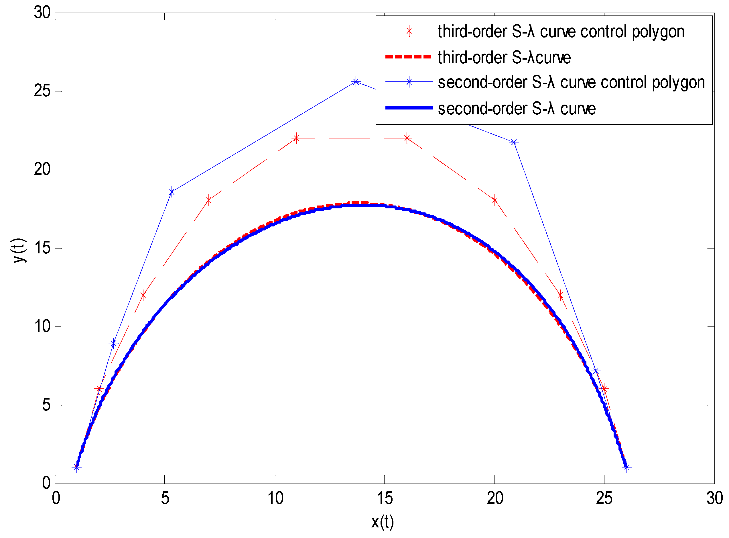
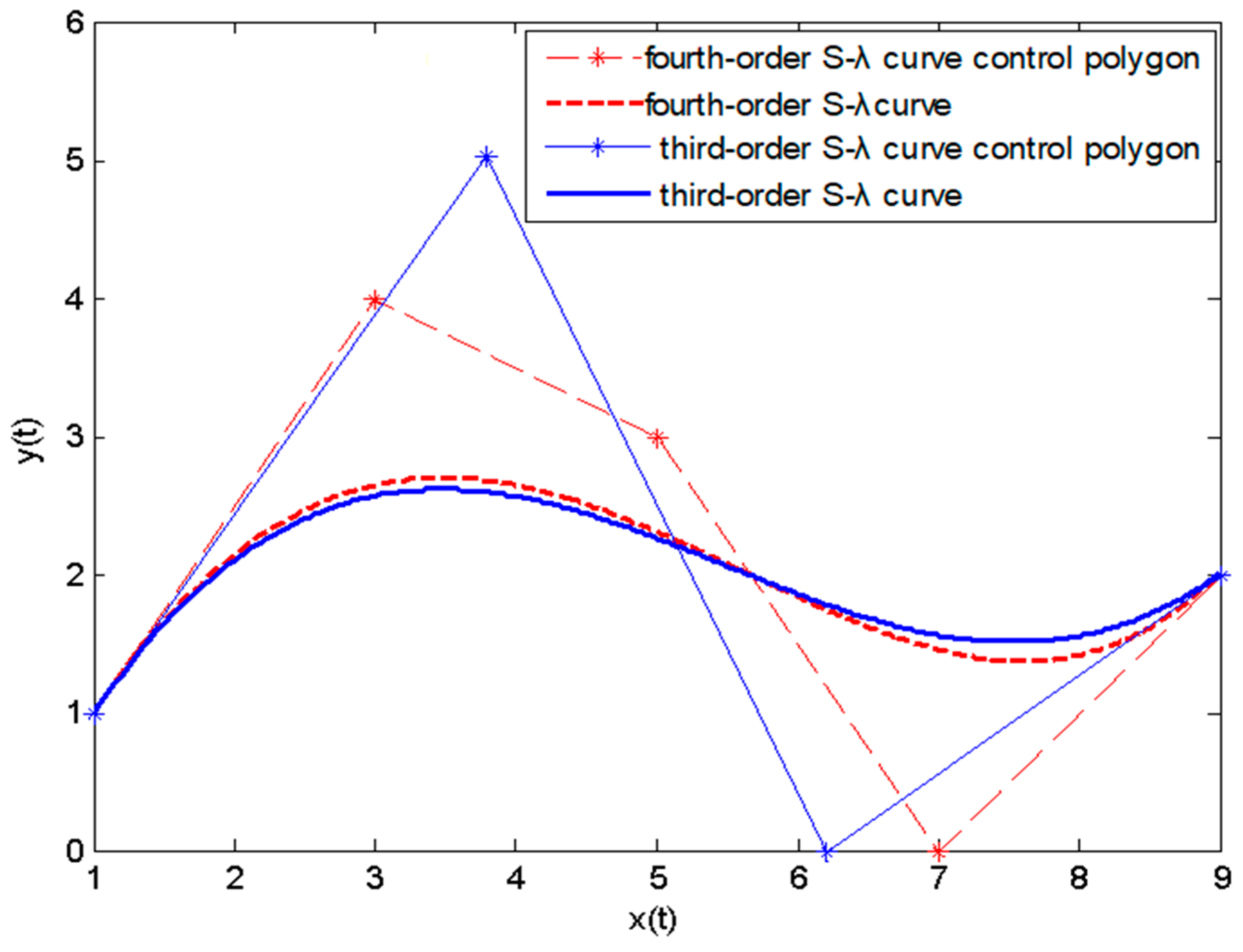
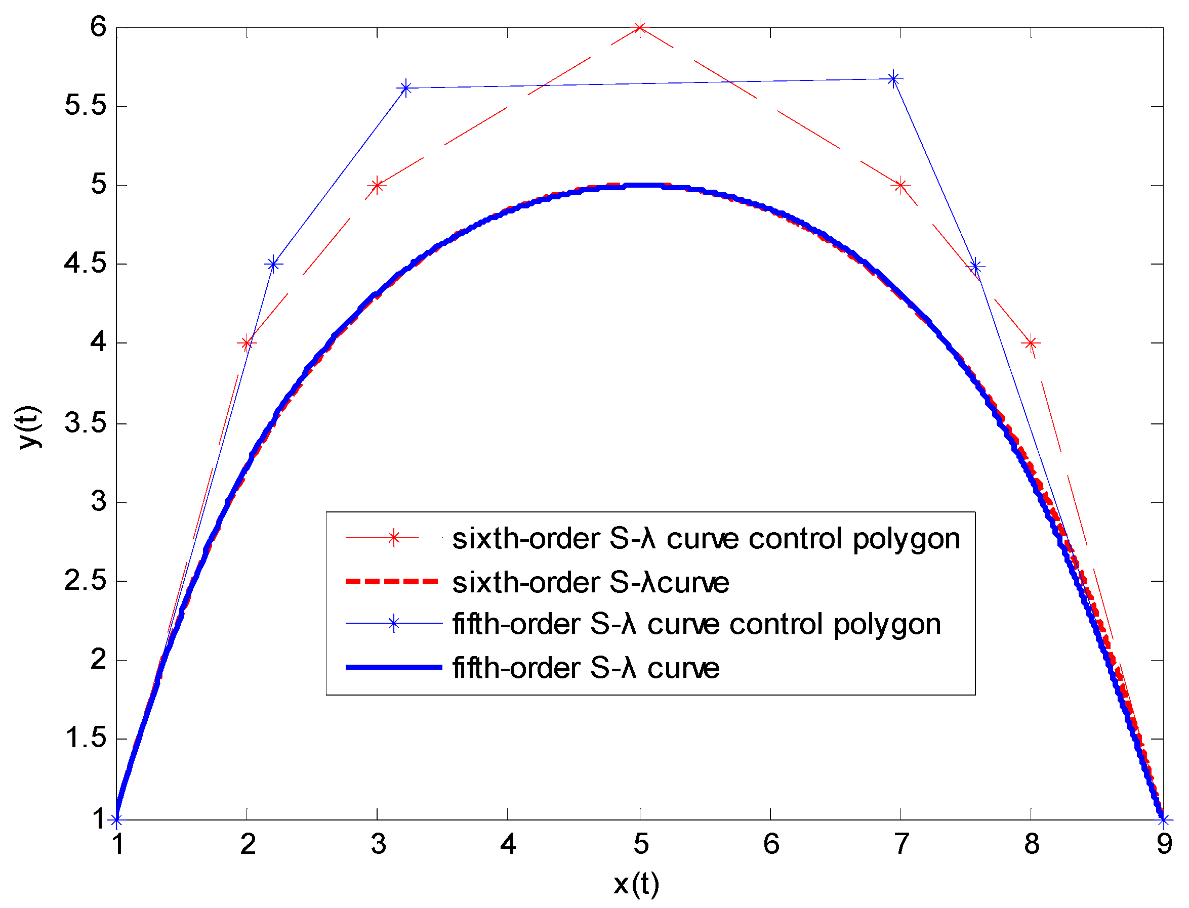
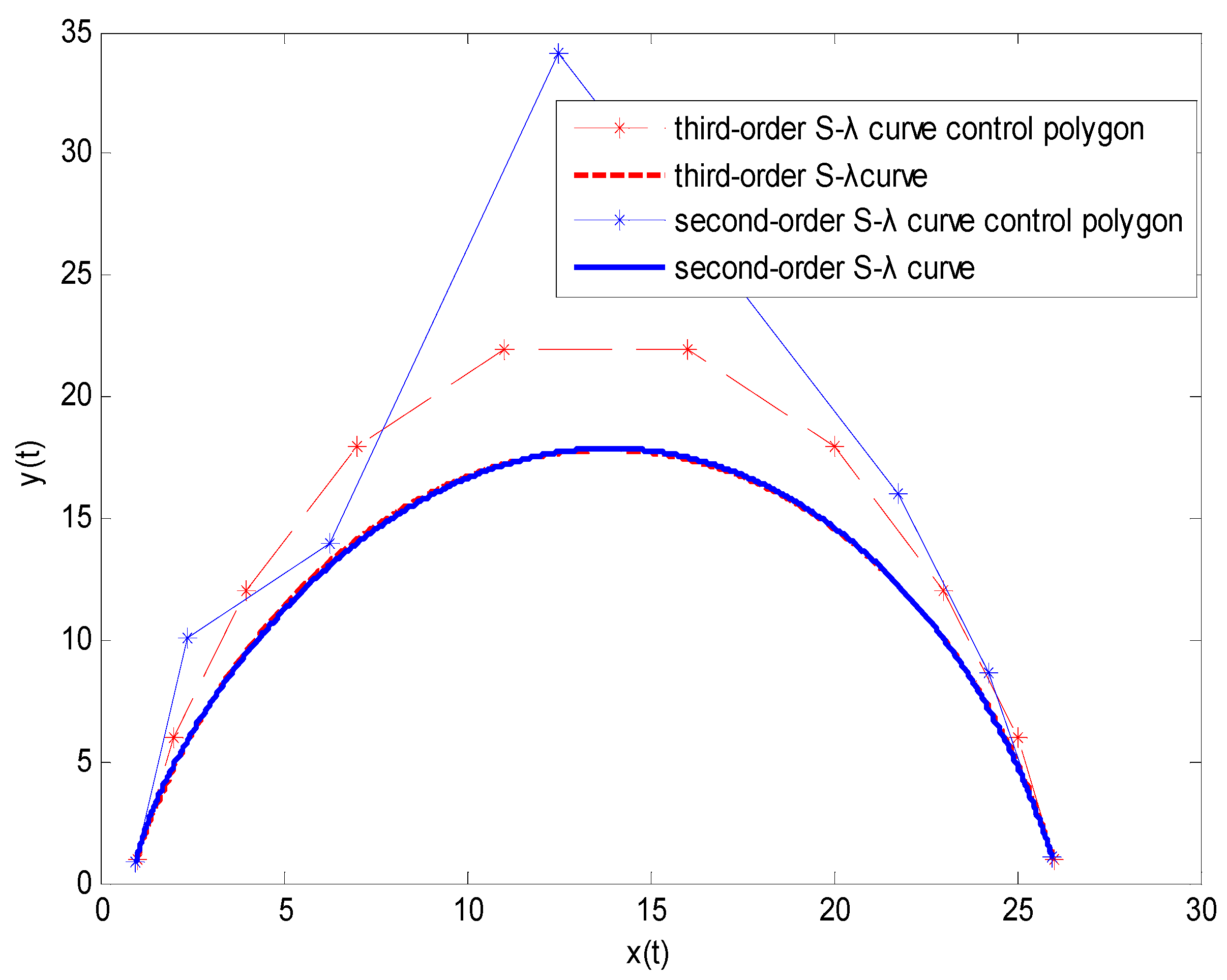
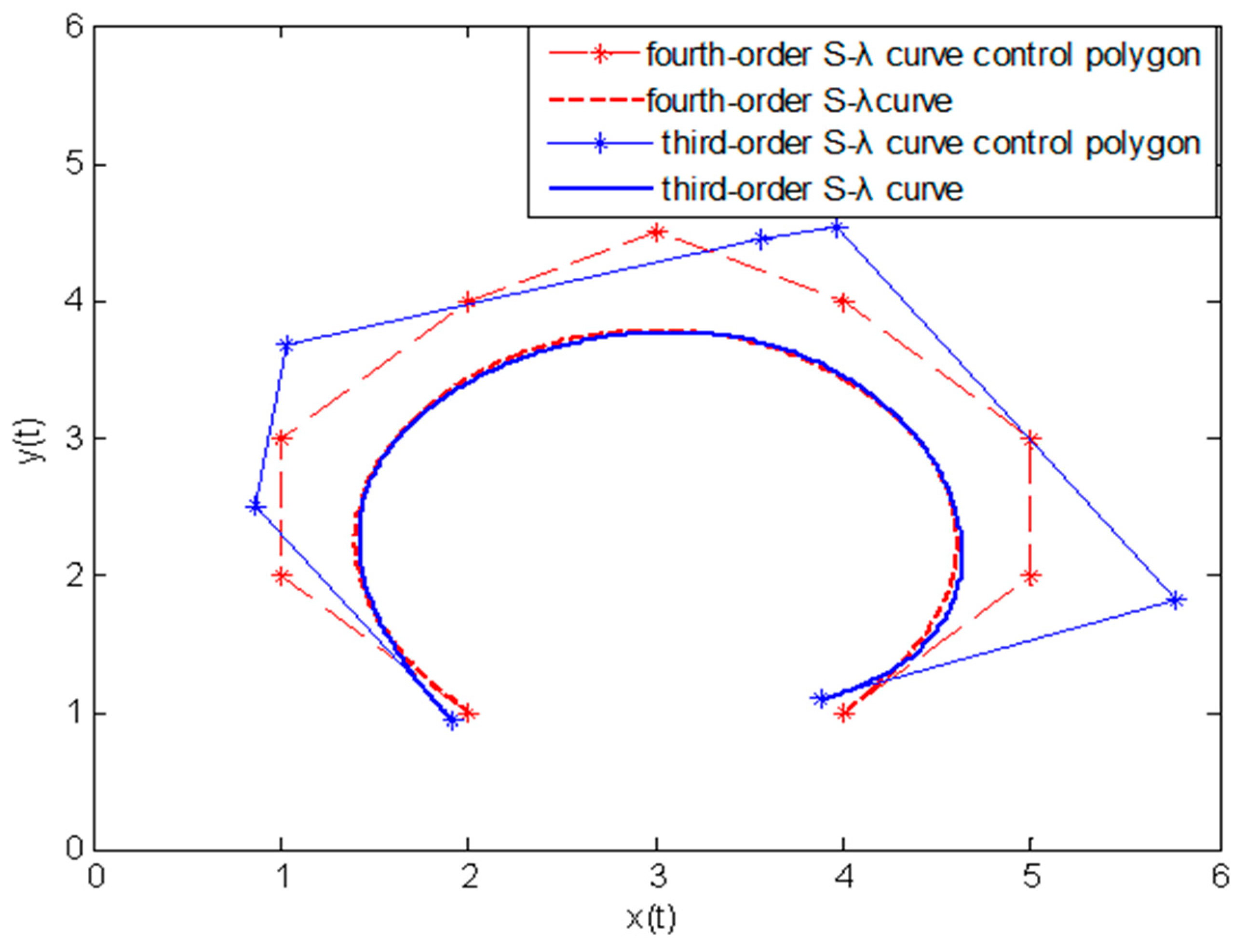
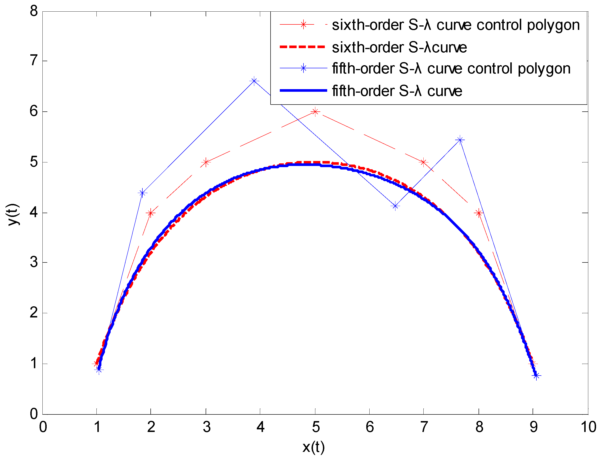
3.4.1. Degree Reduction of S-λ Curves with Fixed Endpoints

Figure 3, Figure 4 and Figure 5 show the result S-λ curves after reducing the degree of the third, fourth and sixth-order S-λ curves, respectively. Note that each group curves in these figures hold fixed endpoints. The control points for the third-order S-λ curve are {(1,1), (2,6), (4,12), (7,18), (11,22), (16,22), (20,18), (23,12), (25,6), (26,1)} and the generating function is $S(x)=1+2x+5x^2+3x^3$. The control points for the fourth-order S-λ curve are {(1,1), (3,4), (5,3), (7,0), (9,2)} and the generating function is $S(x)=1+5x$. The control points for the sixth-order S-λ curve are {(1,1), (2,4), (3,5), (5,6), (7,5), (8,4), (9,1)} and the generating function is $S(x)=1+3x$.

3.4.2. Degree Reduction of S-λ Curves with Unconstrained Endpoint

Figure 6, Figure 7 and Figure 8 show the result S-λ curves obtained by reducing the degree of the third, fourth, and sixth-order S-λ curves using proposed genetic simulated annealing algorithm, respectively. Note that each group curves in these figures possess unconstrained endpoints. The control points for the third-order S-λ curve are {(1,1), (2,6), (4,12), (7,18), (11,22), (16,22), (20,18), (23,12), (25,6), (26,1)} and the generating function is $S(x)=1+2x+5x^2+3x^3$. The control points for the fourth-order S-λ curve are {(2,1), (1,2), (1,3), (2,4), (3,4.5), (4,4), (5,3), (5,2), (4,1)} and the generating function is $S(x)=1+3x+2x^2$. The control points for the sixth-order S-λ curve are {(1,1), (2,4), (3,5), (5,6), (7,5), (8,4), (9,1)} and the generating function is $S(x)=1+3x$.

3.4.3. Quantitative Evaluation of the Degree Reduction Algorithm

The examples discussed in preceding section show that the presented algorithm is valid, which imply that it is a general tool to reduce degree of S-λ curves approximately. In this section we attempt to evaluate its performance objectively based on the error between the degree-reduced curves and the corresponding originals.

Table 1. Error values for degree reduction with fixed endpoints.

Error	Figure 3	Figure 4	Figure 5
$\epsilon$	0.1402	0.9456	0.1914

and

Table 2. Error values for degree reduction with unconstrained endpoints.

Error	Figure 6	Figure 7	Figure 8
$\epsilon$	0.0687	0.2347	0.1903

show the degree reduction errors for the curves shown in Figure 2, Figure 3 and Figure 4 and Figure 5, Figure 6 and Figure 7, respectively. From the tables, we can see that the degree reduction errors of the genetic simulated annealing method are relatively small in all cases, which is consistent with the figures showed in Figure 2, Figure 3, Figure 4, Figure 5, Figure 6 and Figure 7, and means the proposed algorithm is quite effective.

4. Conclusions

This paper presents a new method, which combines the geometric properties of the curves with a new genetic simulated annealing algorithm, to reduce degree of the S-λ curves approximately. The performance of the algorithm is demonstrated by applying it to several examples; the results show that the proposed algorithm can achieve the degree reduction process efficiently and the generated degree-reduced curves are very close to the originals. It is worth noting that the proposed method in this paper is used for approximate degree reduction of S-λ curves for the first time. And we will focus on studying the degree reduction of S-λ surfaces in future work.

References

1. Johnson, N.L.; Kemp, A.W.; Kotz, S. Univariate Discrete Distributions; John Wiley & Sons: New York, NY, USA, 2005. [Google Scholar]
2. Dahmen, W.; Micchelli, C.A. Statistical encounters with B-splines. Contemp. Math. 1986, 59, 17–48. [Google Scholar]
3. Goldman, R.N. Urn models and B-splines. Constr. Approx. 2000, 4, 265–288. [Google Scholar] [CrossRef]
4. Hu, G.; Bo, C.; Wu, J.; Wei, G.; Hou, F. Modeling of Free-Form Complex Curves Using SG-Bézier Curves with Constraints of Geometric Continuities. Symmetry 2018, 10, 545. [Google Scholar] [CrossRef]
5. Hu, G.; Wu, J.L.; Qin, X.Q. A novel extension of the Bézier model and its applications to surface modeling. Adv. Eng. Softw. 2018, 125, 27–54. [Google Scholar] [CrossRef]
6. Hu, G.; Wu, J.L.; Qin, X.Q. A new approach in designing of local controlled developable H-Bézier surfaces. Adv. Eng. Softw. 2018, 121, 26–38. [Google Scholar] [CrossRef]
7. Hu, G.; Cao, H.X.; Zhang, S.X.; Guo, W. Developable Bézier-like surfaces with multiple shape parametersand its continuity conditions. Appl. Math. Model. 2017, 45, 728–747. [Google Scholar] [CrossRef]
8. Goldman, R.N. The rational Bernstein bases and the multirational blossoms. Comput. Aided Geom. Des. 1999, 16, 701–738. [Google Scholar] [CrossRef]
9. Hahn, L. Approximation by operators of probabilistic type. J. Approx. Theory 1980, 30, 1–10. [Google Scholar] [CrossRef]
10. Khan, R.A. Some probabilistic methods in the theory of approximation operators. Acta Math. Sci. Hung. 1980, 35, 193–203. [Google Scholar] [CrossRef]
11. Omey, E. Operators of probabilistic type. Theory Probab. Appl. 1996, 41, 219–225. [Google Scholar] [CrossRef]
12. De La Cal, J. On Stancu-Mühlbach operators and some connected problems concerning probability distributions. J. Approx. Theory 1993, 74, 59–68. [Google Scholar] [CrossRef]
13. Zeng, X.M. Approximation properties of Gamma operators. J. Math. Anal. Appl. 2005, 311, 389–401. [Google Scholar] [CrossRef]
14. Zeng, X.M.; Cheng, F. On the rate of approximation of Bernstein type operators. J. Approx. Theory 2001, 109, 242–256. [Google Scholar] [CrossRef]
15. Fan, F.L.; Zeng, X.M. S-λ bases and S-λ curves. Comput. Aided Des. 2012, 44, 1049–1055. [Google Scholar] [CrossRef]
16. Watkins, M.A.; Worsey, A.J. Degree reduction of Bézier curves. Comput. Aided Des. 1988, 20, 398–405. [Google Scholar] [CrossRef]
17. Lutterkort, D.; Peters, J.; Reif, U. Polynomial degree reduction in the L2-norm equals best Euclidean approximation of Bézier coefficients. Comput. Aided Geom. Des. 1999, 16, 607–612. [Google Scholar] [CrossRef]
18. Ren, S.L.; Zhang, K.Y.; Ye, Z.L. Matrix representation for degree reduction of Bézier curves. J. Eng. Math. 2007, 24, 1007–1014. [Google Scholar]
19. Cai, H.J.; Wang, G.J. Constrained approximation of rational Bézier curves based on a matrix expression of its end points continuity condition. Comput. Aided Des. 2010, 42, 495–504. [Google Scholar] [CrossRef]
20. Ahn, Y.J.; Lee, B.G.; Park, Y.; Yoo, J. Constrained polynomial degree reduction in the L2-norm equals best weighted Euclidean approximation of Bézier coefficients. Comput. Aided Geom. Des. 2004, 21, 181–191. [Google Scholar] [CrossRef]
21. Lu, L.Z.; Hu, Q.Q.; Wang, G.Z. An iterative algorithm for degree reduction of Bézier curves. J. Comput. Aided Des. Comput. Graph. 2009, 21, 1689–1693. [Google Scholar]
22. Lu, L.Z.; Wang, G.Z. Optimal multi-degree reduction of Bézier curves with G2-continuity. Comput. Aided Geom. Des. 2006, 23, 673–683. [Google Scholar] [CrossRef]
23. Delgado, J.; Pena, J.M. Progressive iterative approximation and bases with the fastest convergence rates. Comput. Aided Geom. Des. 2007, 24, 10–18. [Google Scholar] [CrossRef]
24. Ait-Haddou, R.; Bartoň, M. Constrained multi-degree reduction with respect to Jacobi norms. Comput. Aided Geom. Des. 2016, 42, 23–30. [Google Scholar] [CrossRef] [Green Version]
25. Liang, X.X.; Zhang, C.M.; Lin, X. Constrained degree reduction of Bézier curve in L Norm using basic curve and correction curve. J. Comput. Aided Des. Comput. Graph. 2006, 18, 401–405. [Google Scholar]
26. Rababah, A.; Lee, B.G.; Yoo, J. A simple matrix form for degree reduction of Bézier curves using Chebyshev–Bernstein basis transformations. Appl. Math. Comput. 2006, 181, 310–318. [Google Scholar] [CrossRef]
27. Lu, L.Z.; Wang, G.Z. Application of Chebyshev II-Bernstein basis transformations to degree reduction of Bézier curves. J. Comput. Appl. Math. 2008, 221, 52–65. [Google Scholar] [CrossRef]
28. Xu, S.P.; Bai, S.X.; Xiong, Y.H.; Zeng, W. Degree reduction of Bézier curves with constraints of asymmetry parametric endpoints continuity. J. Eng. Graph. 2008, 5, 91–97. [Google Scholar]
29. Wang, W.T. Degree reduction of C-Bézier curves. J. Zhejiang Univ. Sci. A 2009, 36, 396–400. [Google Scholar]
30. Qin, X.Q.; Wang, W.W.; Hu, G. Degree reduction of C-Bézier curve based on genetic algorithm. Comput. Eng. Appl. 2013, 49, 174–181. [Google Scholar]
31. Khuda Bux, N.; Lu, M.; Wang, J.; Hussain, S.; Aljeroudi, Y. Efficient Association Rules Hiding Using Genetic Algorithms. Symmetry 2018, 10, 576. [Google Scholar] [CrossRef]
32. Caponetto, R.; Fortuna, L.; Graziani, S.; Xibilia, M.G. Genetic algorithms and applications in system engineering: A survey. Trans. Inst. Meas. Control 1993, 15, 143–156. [Google Scholar] [CrossRef]
33. Lange, K. Poisson Approximation. In Geometric Modeling and Processing 2000. Theory and Applications. Proceedings; IEEE: Piscataway, NJ, USA, 2000; pp. 141–149. [Google Scholar]
Figure 1. S-λ basis functions in interval [0, 1): Bernstein-Bézier and Szász-Mirakjan, where n = 3.
Symmetry 11 00015 g001
Figure 2. The S-λ curves with same transformation factor and different generating functions.
Symmetry 11 00015 g002
Figure 3. Degree reduction of a third-order S-λ curve with fixed endpoints. The control points of the degree-reduced curve are {(1,1), (2.6958, 8.9393), (5.3362, 18.5222), (13.7203, 25.5980), (20.8985, 21.6798), (24.6082, 7.1808), (26,1)}.
Symmetry 11 00015 g003
Figure 4. Degree reduction of a fourth-order S-λ curve with fixed endpoints. The control points of the degree-reduced curve are {(1,1), (3.7973, 5.0336), (6.2139, 0.0000), (9,2)}.
Symmetry 11 00015 g004
Figure 5. Degree reduction of a sixth-order S-λ curve with fixed endpoints. The control points of the degree-reduced curve are {(1,1), (2.21112, 4.5028), (3.2254, 5.6096), (6.9537, 5.6776), (7.5792, 4.4878), (9,1)}.
Symmetry 11 00015 g005
Figure 6. Degree reduction of a third-order S-λ curve with unconstrained endpoints. The control points of the degree-reduced curve are {(0.9766, 0.8736), (2.3848, 10.1090), (6.2801, 13.9343), (12.4859, 34.1484), (21.7390, 16.0439), (24.2554, 8.6127), (25.9813, 1.0708)}.
Symmetry 11 00015 g006
Figure 7. Degree reduction of a fourth-order S-λ curve with unconstrained endpoints. The control points of the degree-reduced curve are {(1.9132, 0.9329), (0.8636, 2.5036), (1.0289, 3.6672), (3.5579, 4.4441), (3.9541, 4.5389), (5.7761, 1.8075), (3.8825, 1.0933)}.
Symmetry 11 00015 g007
Figure 8. Degree reduction of a sixth-order S-λ curve with unconstrained endpoints. The control points of the degree-reduced curve are {(1.0346, 0.8772), (1.8500, 4.3859), (3.8810, 6.6002), (6.4763, 4.1338), (7.6701, 5.4494), (9.0588, 0.7503)}.
Symmetry 11 00015 g008