Article

Singularities for One-Parameter Developable Surfaces of Curves

1
School of Mathematics and Statistics, Northeast Normal University, Changchun 130024, China
2
School of Mathematics, Jilin University of Finance and Economics, Changchun 130117, China
3
School of Science, Dalian Maritime University, Dalian 116026, China
*
Author to whom correspondence should be addressed.
Symmetry 2019, 11(1), 108; https://doi.org/10.3390/sym11010108
Submission received: 9 January 2019 / Revised: 14 January 2019 / Accepted: 15 January 2019 / Published: 17 January 2019

Abstract

:
Developable surfaces, which are important objects of study, have attracted a lot of attention from many mathematicians. In this paper, we study the geometric properties of one-parameter developable surfaces associated with regular curves. According to singularity theory, the generic singularities of these developable surfaces are classified—they are swallowtails and cuspidal edges. In addition, we give some examples of developable surfaces which have symmetric singularity models.

1. Introduction

The study of developable surfaces has many practical applications. There is much literature about developable surfaces, (see, e.g., [1,2,3,4,5]). Many cartographic projections involve projecting the Earth onto a developable surface and then “unrolling” the surface into a region on the plane. Since developable surfaces may be constructed by bending flat sheets, they are also important in manufacturing objects from cardboard, plywood, and sheet metal. In mathematics, developable surfaces are typically defined as surfaces which can be developed into planes without distorting the surface metric. There is some literature about developable surfaces of space curves from the viewpoint of singularity theory [1,2]. The tangent developable surface of a space curve is a ruled surface, which is formed by the space curve’s tangent lines. In algebraic geometry, tangent developable surfaces play an important role in the duality theory [6]. In [1], the author investigated the relationship between the singularities of tangent developable surfaces and some types of space curves. He also gave a classification of tangent developable surfaces by using the local topological property. On the other hand, S. Izumiya et al. introduced the rectifying developable surfaces of space curves in [2], where they showed that a regular curve is a geodesic of its rectifying developable surface and revealed the relationship between singularities of the rectifying developable surface and geometric invariants. The geometric invariants can also characterize the contact between a space curve and a helix. In this sense, the study of the singularities of developable surfaces is an interesting subject.
In the present paper, we investigate one-parameter developable surfaces, which are related to the space curves, as a fundamental case for the research of the highest dimensional manifolds in Euclidean 3-space. We investigated the singularities of hypersurfaces in semi-Euclidean space [7,8,9,10]. However, at least to the best of our knowledge, there exists little literature concerning the singularities of one-parameter developable surfaces related to regular space curves in Euclidean space. Therefore, we study this problem in the present paper. In the frame of space curves, we define one-parameter developable surfaces. When the parameter is fixed, the sections of one-parameter developable surfaces are developable surfaces. Moreover, the tangent developable surfaces and the rectifying developable surfaces are sections of one-parameter developable surfaces. We also define the one-parameter support functions on regular space curves, which can be used to study the geometric properties of one-parameter developable surfaces. In fact, one-parameter developable surfaces are the discriminant sets of these functions. The main result, Theorem 2, shows that the singularities of developable surfaces are A k -singularities ( k = 2 , 3 ) of these functions.
The organization of this paper is as follows: We review the concepts of ruled surfaces in Euclidean space in Section 2. In Section 3, the one-parameter developable surfaces of a space curve are defined, and we obtain two geometric invariants of the curve. We also get singularities of one-parameter developable surfaces (Theorem 1), and Theorem 2 gives the classification of these singularities in this section. The preparations for the proof of Theorem 2 are in Section 4 and Section 5. In the last section, we give some examples to illustrate the main results in this paper.

2. Basic Notation

Let R 3 be 3-dimensional Euclidean space and x = ( x 1 , x 2 , x 3 ) , y = ( y 1 , y 2 , y 3 ) R 3 . We denote their standard inner product by x · y , and the norm of x is denoted by x . Let γ : I R 3 be a curve and the tangent vector respect to t is γ ˙ ( t ) = d γ / d t ( t ) . The arc-length is s ( t ) = t 0 t γ ˙ ( t ) d t and γ ( s ) = d γ / d s = 1 . We define three unit vectors t ( s ) = γ ( s ) , n ( s ) = γ ( s ) / γ ( s ) , and b ( s ) = t ( s ) × n ( s ) . Then, the Frenet-Serret formula is as follows:
t ( s ) = κ ( s ) n ( s ) n ( s ) = κ ( s ) t ( s ) + τ ( s ) b ( s ) b ( s ) = τ ( s ) n ( s ) ,
where κ ( s ) is the curvature function and τ ( s ) is the torsion function.
We now introduce developable surfaces and ruled surfaces. Suppose that γ : I R 3 be a curve and ξ : I R 3 { 0 } be a C -mapping. A surface F ( γ , ξ ) : I × R R 3 is defined by
F ( γ , ξ ) ( s , u ) = γ ( s ) + u ξ ( s ) ,
then F ( γ , ξ ) is a ruled surface, and γ and ξ are called the base curve and director curve, respectively. For a fixed s I , γ ( s ) + u ξ ( s ) is the ruling. A developable surface is a ruled surface with vanishing Gaussian curvature. It’s well known that F ( γ , ξ ) is a developable surface if and only if det ( γ ( s ) , ξ ( s ) , ξ ( s ) ) = 0 .
F ( γ , ξ ) is called a cylinder if the director curve ξ has a fixed direction. We denote that ξ ˜ ( s ) = ξ ( s ) / ξ ( s ) , then F ( γ , ξ ) is a cylinder if and only if ξ ˜ ( s ) 0 . If a ruled surface F ( γ , ξ ) is not a cylinder, a striction curve of F ( γ , ξ ) is defined by
c ( s ) = γ ( s ) γ ( s ) · ξ ˜ ( s ) ξ ˜ ( s ) · ξ ˜ ( s ) ξ ˜ ( s ) .
It is known that the singularities of ruled surface F ( γ , ξ ) (not a cylinder) are located on its striction curve [11]. We say F ( γ , ξ ) is a cone if and only if the striction curve c is constant.

3. One-Parameter Developable Surfaces

We consider the one-parameter developable surfaces of space curves in this section. Let γ be a space curve. We consider a spherical vector L : [ 0 , π 2 ] × I S 2 , which is defined by
L ( s , θ ) = τ ( s ) t ( s ) κ ( s ) sin θ cos θ n ( s ) + κ ( s ) cos 2 θ b ( s ) τ 2 ( s ) + κ 2 ( s ) cos 2 θ ,
where τ 2 ( s ) + κ 2 ( s ) cos 2 θ 0 . We assume, throughout the whole paper, that τ 2 ( s ) + κ 2 ( s ) cos 2 θ 0 for any ( s , θ ) I × [ 0 , π 2 ] . We write L ( s , θ ) = L θ ( s ) , and define a map D θ : I × R R 3 by
D θ ( s , u ) = γ ( s ) + u L θ ( s ) = γ ( s ) + u τ ( s ) t ( s ) κ ( s ) sin θ cos θ n ( s ) + κ ( s ) cos 2 θ b ( s ) τ 2 ( s ) + κ 2 ( s ) cos 2 θ .
We call D θ a one-parameter developable surface of γ . We can easily check that D π 2 ( s , u ) is the tangent developable surface of γ and D 0 ( s , u ) is the rectifying developable surface of γ .
For any θ 0 [ 0 , π 2 ] , we have
L θ 0 ( s ) = ( κ τ 2 sin θ 0 + κ 3 sin θ 0 cos 2 θ 0 + κ τ cos θ 0 κ τ cos θ 0 ) ( κ cos θ 0 t + τ sin θ 0 n τ cos θ 0 b ) ( τ 2 + κ 2 cos 2 θ 0 ) 3 2 .
So, we have
det γ ( s ) , L θ 0 ( s ) , L θ 0 ( s ) = κ τ 2 sin θ 0 + κ 3 sin θ 0 cos 2 θ 0 + κ τ cos θ 0 κ τ cos θ 0 det ( t , τ t κ sin θ 0 cos θ 0 n + κ cos 2 θ 0 b τ 2 + κ 2 cos 2 θ 0 , κ cos θ 0 t + τ sin θ 0 n τ cos θ 0 b ( τ 2 + κ 2 cos 2 θ 0 ) 3 2 ) = 0
for all s I . This means D θ 0 is a developable surface. For this reason, we call D θ the one-parameter developable surfaces of γ . Moreover, we introduce two invariants as follows:
δ ( s ) = κ ( s ) sin θ 0 ( τ 2 ( s ) + κ 2 ( s ) cos 2 θ 0 ) + cos θ 0 ( κ ( s ) τ ( s ) κ ( s ) τ ( s ) ) τ 2 ( s ) + κ 2 ( s ) cos 2 θ 0 , σ ( s ) = τ ( s ) τ 2 ( s ) + κ 2 ( s ) cos 2 θ 0 d d s κ ( s ) cos θ 0 δ ( s ) τ 2 ( s ) + κ 2 ( s ) cos 2 θ 0 , ( when δ ( s ) 0 ) .
Since
L θ 0 ( s ) = ( κ τ 2 sin θ 0 + κ 3 sin θ 0 cos 2 θ 0 + κ τ cos θ 0 κ τ cos θ 0 ) ( κ cos θ 0 t + τ sin θ 0 n τ cos θ 0 b ) ( τ 2 + κ 2 cos 2 θ 0 ) 3 2 ( s ) = δ ( s ) κ cos θ 0 t + τ sin θ 0 n τ cos θ 0 b τ 2 + κ 2 cos 2 θ 0 ( s ) ,
so that δ ( s ) = 0 if and only if L θ 0 ( s ) = 0 . We can also calculate that
D θ 0 s ( s , u ) × D θ 0 u ( s , u ) = κ ( s ) cos θ 0 τ 2 ( s ) + κ 2 ( s ) cos 2 θ 0 + u δ ( s ) ( sin θ 0 b ( s ) + cos θ 0 n ( s ) ) .
Thus, that ( s 0 , u 0 ) I × R is a singular point of D θ 0 is equivalent to
κ ( s 0 ) cos θ 0 τ 2 ( s 0 ) + κ 2 ( s 0 ) cos 2 θ 0 + u 0 κ ( s 0 ) sin θ 0 ( τ 2 ( s 0 ) + κ 2 ( s 0 ) cos 2 θ 0 ) + cos θ 0 ( κ ( s 0 ) τ ( s 0 ) κ ( s 0 ) τ ( s 0 ) ) τ 2 ( s 0 ) + κ 2 ( s 0 ) cos 2 θ 0 = 0 .
If θ 0 π 2 and ( s 0 , u 0 ) is a singular point of D θ 0 , then we have u 0 0 ; that is, D θ 0 has no singular points on the base curve γ ( s ) . We have the following result for δ ( s ) and σ ( s ) :
Theorem 1.
Let γ : I R 3 be a unit speed curve. Then the following holds:
(A) For any θ 0 [ 0 , π 2 ] , the following statements are equivalent:
(1) 
D θ 0 is a cylinder,
(2) 
δ ( s ) = 0 for all s I .
(B) If δ ( s ) 0 for all s I , then the following statements are equivalent:
(3) 
D θ 0 is a conical surface,
(4) 
σ ( s ) = 0 for all s I .
(C) The singularities of one-parameter developable surfaces D θ are γ ( s ) , D π 2 and
{ D θ ( s , u ) | κ ( s ) cos θ τ 2 ( s ) + κ 2 ( s ) cos 2 θ + u [ κ ( s ) sin θ ( τ 2 ( s ) + κ 2 ( s ) cos 2 θ ) + cos θ ( κ ( s ) τ ( s ) κ ( s ) τ ( s ) ) ] = 0 } .
Proof. 
(A) By definition, the developable surface is a cylinder if and only if the director vector is a constant vector and L θ 0 ( s ) is the director vector of D θ 0 . Since
L θ 0 ( s ) = δ ( s ) κ cos θ 0 t + τ sin θ 0 n τ cos θ 0 b τ 2 + κ 2 cos 2 θ 0 ( s ) ,
then D θ 0 is a cylinder if and only if δ ( s ) = 0 for all s I .
(B) We consider the striction curve c ( s ) which is defined by
c ( s ) = γ ( s ) γ ( s ) · L θ 0 ( s ) L θ 0 ( s ) · L θ 0 ( s ) L θ 0 ( s ) = γ ( s ) κ ( s ) cos θ 0 δ ( s ) τ 2 ( s ) + κ 2 ( s ) cos 2 θ 0 L θ 0 ( s ) .
Then (B)-(3) is equivalent to c ( s ) = 0 , for all s I . We can calculate that
c = γ d d s κ cos θ 0 δ τ 2 + κ 2 cos 2 θ 0 L θ 0 κ cos θ 0 δ τ 2 + κ 2 cos 2 θ 0 L θ 0 = t κ cos θ 0 δ τ 2 + κ 2 cos 2 θ 0 δ ( κ cos θ 0 t + τ sin θ 0 n τ cos θ 0 b ) τ 2 + κ 2 cos 2 θ 0 d d s κ cos θ 0 δ τ 2 + κ 2 cos 2 θ 0 L θ 0 = τ ( τ t κ cos θ 0 sin θ 0 n + κ cos 2 θ 0 b ) τ 2 + κ 2 cos 2 θ 0 d d s κ cos θ 0 δ τ 2 + κ 2 cos 2 θ 0 L θ 0 = σ ( s ) L θ 0 .
It follows that (B)-(3) and (B)-(4) are equivalent.
(C) By straightforward calculation, we have
D θ s = t + u [ κ sin θ ( τ 2 + κ 2 cos 2 θ ) + cos θ ( κ τ κ τ ) ] ( τ sin θ n + κ cos θ t τ cos θ b ) ( τ 2 + κ 2 cos 2 θ ) 3 2 , D θ u = τ t κ sin θ cos θ n + κ cos 2 θ b τ 2 + κ 2 cos 2 θ , D θ θ = u κ 2 τ cos θ sin θ t + ( κ τ 2 sin 2 θ κ 3 cos 4 θ κ τ 2 cos 2 θ ) n ( κ 3 sin θ cos 3 θ + 2 κ τ 2 cos θ sin θ ) b ( τ 2 + κ 2 cos 2 θ ) 3 2 .
We can obtain the singularities of D θ if the above three vectors are linearly dependent, which is equivalent to
u κ cos θ [ u ( κ sin θ ( τ 2 + κ 2 cos 2 θ ) + cos θ ( κ τ κ τ ) ) + κ cos θ τ 2 + κ 2 cos 2 θ ] ( τ 2 + κ 2 cos 2 θ ) 3 2 = 0 .
This means that u = 0 or cos θ = 0 or
κ ( s ) cos θ τ 2 ( s ) + κ 2 ( s ) cos 2 θ + u [ sin θ κ ( s ) ( τ 2 ( s ) + κ 2 ( s ) cos 2 θ ) cos θ ( κ ( s ) τ ( s ) κ ( s ) τ ( s ) ) ] = 0 .
Therefore, (C) holds.  □
We give relationships between the singularities of one-parameter developable surfaces of unit speed curves and the above two invariants, as follows:
Theorem 2.
Let γ : I R 3 be a space curve. Then, we have the following:
(1) ( s 0 , u 0 ) is a regular point of D θ 0 if and only if
u 0 δ ( s 0 ) + κ ( s 0 ) cos θ 0 τ 2 ( s 0 ) + κ 2 ( s 0 ) cos 2 θ 0 0 .
(2) Suppose ( s 0 , u 0 ) is a singular point of D θ 0 , then D θ 0 is locally diffeomorphic to the cuspidal edge at ( s 0 , u 0 ) if
(i) 
δ ( s 0 ) 0 , σ ( s 0 ) 0 and
u 0 = κ ( s 0 ) cos θ 0 δ ( s 0 ) τ 2 ( s 0 ) + κ 2 ( s 0 ) cos 2 θ 0 ,
or
(ii) 
δ ( s 0 ) = cos θ 0 = 0 and
u 0 κ ( s 0 ) τ ( s 0 ) κ ( s 0 ) τ ( s 0 ) + κ ( s 0 ) τ ( s 0 ) .
(3) Suppose ( s 0 , u 0 ) is a singular point of D θ 0 , then D θ 0 is locally diffeomorphic to the swallowtail at ( s 0 , u 0 ) if δ ( s 0 ) 0 , σ ( s 0 ) = 0 , σ ( s 0 ) 0 and
u 0 = κ ( s 0 ) cos θ 0 δ ( s 0 ) τ 2 ( s 0 ) + κ 2 ( s 0 ) cos 2 θ 0 .
Here S W = { ( x 1 , x 2 , x 3 ) | x 1 = 3 u 4 + u 2 v , x 2 = 4 u 3 + 2 u v , x 3 = v } is the swallowtail, C = { ( x 1 , x 2 , x 3 ) | x 1 2 = x 2 3 } is the cusp and C × R is the cuspidal edge (see Figure 1, Figure 2 and Figure 3).

4. One-Parameter Support Functions

For a space curve γ : I R 3 , we introduce a function
G : I × [ 0 , π 2 ] × R 3 R
by G ( s , θ , x ) = cos θ n ( s ) + sin θ b ( s ) · x γ ( s ) . G is called the one-parameter support function of γ , with respect to the unit normal vector cos θ n ( s ) + sin θ b ( s ) . We denote g θ 0 , x 0 ( s ) = G ( s , θ 0 , x 0 ) for any ( θ 0 , x 0 ) [ 0 , π 2 ] × R 3 . Then, we have the following proposition:
Proposition 3.
Let γ : I R 3 be a unit speed curve and g θ 0 , x 0 ( s ) = x 0 γ ( s ) · cos θ 0 n ( s ) + sin θ 0 b ( s ) the one-parameter support function. Then, the following statements hold:
(1) g θ 0 , x 0 ( s 0 ) = 0 if and only if there exist v , u R such that
x 0 γ ( s 0 ) = u t ( s 0 ) + v sin θ 0 n ( s 0 ) cos θ 0 b ( s 0 ) .
(2) g θ 0 , x 0 ( s 0 ) = g θ 0 , x 0 ( s 0 ) = 0 if and only if there exists u R , such that
x 0 γ ( s 0 ) = u τ ( s 0 ) t ( s 0 ) κ ( s 0 ) sin θ 0 cos θ 0 n ( s 0 ) + κ ( s 0 ) cos 2 θ 0 b ( s 0 ) τ 2 ( s 0 ) + κ 2 ( s 0 ) cos 2 θ 0 .
(A) Suppose δ ( s 0 ) 0 . Then, we have the following:
(3) g θ 0 , x 0 ( s 0 ) = g θ 0 , x 0 ( s 0 ) = g θ 0 , x 0 ( s 0 ) = 0 if and only if
x 0 γ ( s 0 ) = κ ( s 0 ) cos θ 0 δ ( s 0 ) τ 2 ( s 0 ) + κ 2 ( s 0 ) cos 2 θ 0 t ( s 0 ) τ ( s 0 ) κ ( s 0 ) sin θ 0 cos θ 0 n ( s 0 ) + κ ( s 0 ) cos 2 θ 0 b ( s 0 ) κ 2 ( s 0 ) cos 2 θ 0 + τ 2 ( s 0 ) .
(4) g θ 0 , x 0 ( s 0 ) = g θ 0 , x 0 ( s 0 ) = g θ 0 , x 0 ( s 0 ) = g θ 0 , x 0 ( 3 ) ( s 0 ) = 0 if and only if σ ( s 0 ) = 0 and
x 0 γ ( s 0 ) = κ ( s 0 ) cos θ 0 δ ( s 0 ) τ 2 ( s 0 ) + κ 2 ( s 0 ) cos 2 θ 0 τ ( s 0 ) t ( s 0 ) κ ( s 0 ) sin θ 0 cos θ 0 n ( s 0 ) + κ ( s 0 ) cos 2 θ 0 b ( s 0 ) κ 2 ( s 0 ) cos 2 θ 0 + τ 2 ( s 0 ) .
(5) g θ 0 , x 0 ( s 0 ) = g θ 0 , x 0 ( s 0 ) = g θ 0 , x 0 ( s 0 ) = g θ 0 , x 0 ( 3 ) ( s 0 ) = g θ 0 , x 0 ( 4 ) ( s 0 ) = 0 if and only if σ ( s 0 ) = σ ( s 0 ) = 0 and
x 0 γ ( s 0 ) = κ ( s 0 ) cos θ 0 δ ( s 0 ) κ 2 ( s 0 ) cos 2 θ 0 + τ 2 ( s 0 ) τ ( s 0 ) t ( s 0 ) κ ( s 0 ) sin θ 0 cos θ 0 n ( s 0 ) + κ ( s 0 ) cos 2 θ 0 b ( s 0 ) τ 2 ( s 0 ) + κ 2 ( s 0 ) cos 2 θ 0 .
(B) Suppose δ ( s 0 ) = 0 . Then, the following statements hold:
(6) g θ 0 , x 0 ( s 0 ) = g θ 0 , x 0 ( s 0 ) = g θ 0 , x 0 ( s 0 ) = 0 if and only if cos θ 0 = 0 ( θ 0 = π 2 ) and there exists u R , such that
x 0 γ ( s 0 ) = u t ( s 0 ) .
(7) g θ 0 , x 0 ( s 0 ) = g θ 0 , x 0 ( s 0 ) = g θ 0 , x 0 ( s 0 ) = g θ 0 , x 0 ( 3 ) ( s 0 ) = 0 if and only if cos θ 0 = 0 ( θ 0 = π 2 ) and
x 0 γ ( s 0 ) = κ ( s 0 ) τ ( s 0 ) κ ( s 0 ) τ ( s 0 ) + κ ( s 0 ) τ ( s 0 ) t ( s 0 ) .
Proof. 
Since g θ 0 , x 0 ( s ) = x 0 γ ( s ) · cos θ 0 n ( s ) + sin θ 0 b ( s ) , we have the following:
( i ) g θ 0 , x 0 = ( x 0 γ ) · ( κ cos θ 0 t + τ cos θ 0 b τ sin θ 0 n ) , ( i i ) g θ 0 , x 0 = κ cos θ 0 + ( x 0 γ ) · [ ( κ τ sin θ 0 κ cos θ 0 ) t ( τ 2 cos θ 0 + κ 2 cos θ 0 + τ sin θ 0 ) n ( τ 2 sin θ 0 τ cos θ 0 ) b ] , ( i i i ) g θ 0 , x 0 = 2 κ cos θ 0 κ τ sin θ 0 + ( x 0 γ ) · [ ( κ τ sin θ 0 κ cos θ 0 + κ τ sin θ 0 + κ τ 2 cos θ 0 + κ 3 cos θ 0 ) t + ( κ 3 τ sin θ 0 3 τ τ cos θ 0 3 κ κ cos θ 0 τ sin θ 0 + τ 3 sin θ 0 ) n + ( τ cos θ 0 κ 2 τ cos θ 0 3 τ τ sin θ 0 τ 3 cos θ 0 ) b ] , ( i v ) g θ 0 , x 0 ( 4 ) = 3 κ cos θ 0 2 κ τ sin θ 0 κ 3 cos θ 0 2 κ τ sin θ 0 κ τ 2 cos θ 0 + ( x 0 γ ) · [ ( κ τ sin θ 0 κ cos θ 0 + 2 κ τ sin θ 0 + κ τ 2 cos θ 0 + 2 κ τ sin θ 0 + 6 κ 2 κ cos θ 0 κ 4 τ sin θ 0 κ τ 3 sin θ 0 + 5 κ τ τ cos θ 0 ) t + ( κ κ τ sin θ 0 4 κ κ cos θ 0 + κ 2 τ sin θ 0 + κ 4 cos θ 0 + 2 κ 2 τ 2 cos θ 0 + 3 κ 2 κ τ sin θ 0 + κ 3 τ sin θ 0 4 τ τ cos θ 0 3 ( κ ) 2 cos θ 0 3 ( τ ) 2 cos θ 0 + τ 4 cos θ 0 + 6 τ 2 τ sin θ 0 ) n + ( τ cos θ 0 3 ( τ ) 2 sin θ 0 4 τ τ sin θ 0 5 κ κ τ cos θ 0 κ 2 τ cos θ 0 + τ 4 sin θ 0 6 τ 2 τ cos θ 0 κ 3 τ 2 sin θ 0 ) b ] .
By definition, g θ 0 , x 0 ( s 0 ) = 0 if and only if x 0 γ ( s 0 ) = u t ( s 0 ) + a n ( s 0 ) + b b ( s 0 ) and a cos θ 0 + b sin θ 0 = 0 , where u , a , b R . We write a = v sin θ 0 and b = v cos θ 0 , where v is a real number. Then, we have
x 0 γ ( s 0 ) = u t ( s 0 ) + v sin θ 0 n ( s 0 ) cos θ 0 b ( s 0 ) .
Therefore, (1) holds.
By (i), g θ 0 , x 0 ( s 0 ) = g θ 0 , x 0 ( s 0 ) = 0 if and only if
x 0 γ ( s 0 ) = u t ( s 0 ) + v sin θ 0 n ( s 0 ) cos θ 0 b ( s 0 )
and u κ cos θ 0 + v τ = 0 . Since κ 0 and κ 2 cos θ 0 2 + τ 2 0 , then there exists u R such that
x 0 γ ( s 0 ) = u τ ( s 0 ) t ( s 0 ) κ ( s 0 ) sin θ 0 cos θ 0 n ( s 0 ) + cos 2 θ 0 κ ( s 0 ) b ( s 0 ) τ 2 ( s 0 ) + κ 2 ( s 0 ) cos 2 θ 0 .
Therefore, (2) holds.
By (ii), g θ 0 , x 0 ( s 0 ) = g θ 0 , x 0 ( s 0 ) = g θ 0 , x 0 ( s 0 ) = 0 if and only if there exists u R , such that
x 0 γ ( s 0 ) = u τ ( s 0 ) t ( s 0 ) κ ( s 0 ) sin θ 0 cos θ 0 n ( s 0 ) + κ ( s 0 ) cos 2 θ 0 b ( s 0 ) τ 2 ( s 0 ) + κ 2 ( s 0 ) cos 2 θ 0
and
κ ( s 0 ) cos θ 0 + u κ ( s 0 ) sin θ 0 ( τ 2 ( s 0 ) + κ 2 ( s 0 ) cos 2 θ 0 ) cos θ 0 ( κ ( s 0 ) τ ( s 0 ) κ ( s 0 ) τ ( s 0 ) ) κ 2 ( s 0 ) cos 2 θ 0 + τ 2 ( s 0 ) = 0 .
It follows
κ ( s 0 ) cos θ 0 + u δ ( s 0 ) κ 2 ( s 0 ) cos 2 θ 0 + τ 2 ( s 0 ) = 0 .
Thus,
δ ( s 0 ) = κ ( s 0 ) sin θ 0 ( κ 2 ( s 0 ) cos 2 θ 0 + τ 2 ( s 0 ) ) cos θ 0 ( κ ( s 0 ) τ ( s 0 ) κ ( s ) τ ( s 0 ) ) κ 2 ( s 0 ) cos 2 θ 0 + τ 2 ( s 0 ) 0
and
u = κ ( s 0 ) cos θ 0 δ ( s 0 ) τ 2 ( s 0 ) + κ 2 ( s 0 ) cos 2 θ 0 ,
or δ ( s 0 ) = 0 and cos θ 0 = 0 . This completes the proof of (A)-(3) and (B)-(6).
Suppose δ ( s 0 ) 0 . By (iii), we have
g θ 0 , x 0 ( s 0 ) = g θ 0 , x 0 ( s 0 ) = g θ 0 , x 0 ( s 0 ) = g θ 0 , x 0 ( s 0 ) = 0
if and only if
x 0 γ ( s 0 ) = κ ( s 0 ) cos θ 0 δ ( s 0 ) κ 2 ( s 0 ) cos 2 θ 0 + τ 2 ( s 0 ) t ( s 0 ) τ ( s 0 ) κ ( s 0 ) sin θ 0 cos θ 0 n ( s 0 ) + κ ( s 0 ) cos 2 θ 0 b ( s 0 ) τ 2 ( s 0 ) + κ 2 ( s 0 ) cos 2 θ 0
and
[ 2 κ cos θ 0 κ τ sin θ 0 κ cos θ 0 δ ( τ 2 + κ 2 cos 2 θ 0 ) ( κ τ 2 sin θ 0 + 2 κ τ τ sin θ 0 + 3 κ 2 κ sin θ 0 cos 2 θ 0 τ κ cos θ 0 + κ τ cos θ 0 ) ] ( s 0 ) = 0 .
We rewrite σ ( s ) as following:
σ ( s ) = τ 2 + κ 2 cos 2 θ 0 [ 2 κ cos θ 0 κ τ sin θ 0 κ cos θ 0 δ ( τ 2 + κ 2 cos 2 θ 0 ) ( κ τ 2 sin θ 0 + 3 κ 2 κ sin θ 0 cos 2 θ 0 + 2 κ τ τ sin θ 0 τ κ cos θ 0 + κ τ cos θ 0 ) ] ( s ) .
Therefore, we have (A)-(4). By similar arguments as above, we have (A)-(5).
Suppose δ ( s 0 ) = 0 . By (iii), g θ 0 , x 0 ( s 0 ) = g θ 0 , x 0 ( s 0 ) = g θ 0 , x 0 ( s 0 ) = g θ 0 , x 0 ( s 0 ) = 0 if and only if cos θ 0 = 0 and
κ ( s 0 ) τ ( s 0 ) + u κ ( s 0 ) τ ( s 0 ) + κ ( s 0 ) τ ( s 0 ) = 0 ,
where u R . Since τ 2 ( s 0 ) + κ 2 ( s 0 ) cos 2 θ 0 0 and cos θ 0 = 0 , we have u = κ ( s 0 ) τ ( s 0 ) κ ( s 0 ) τ ( s 0 ) + κ ( s 0 ) τ ( s 0 ) . Therefore, we obtain (B)-(7).  □

5. Unfoldings of One-Parameter Support Functions

In this section, by using the unfolding theory of functions, we give a classification for singularities of the one-parameter developable surface of γ .
Suppose that F : ( R × R r , ( s 0 , x 0 ) ) R be a function germ, and write f ( s ) = F x 0 ( s , x 0 ) . F is called an r- p a r a m e t e r u n f o l d i n g of f. We say that f has an A k -singularity at s 0 if f ( p ) ( s 0 ) = 0 , for all 1 p k and f ( k + 1 ) ( s 0 ) 0 . If f ( p ) ( s 0 ) = 0 , for all 1 p k , we also say that f has an A k -singularity at s 0 . Suppose f has an A k -singularity ( k 1 ) at s 0 and F be an r-parameter unfolding of f; then, we write the ( k 1 ) -jet of F / x i at s 0 as
j ( k 1 ) F x i ( s , x 0 ) ( s 0 ) = j = 1 k + 1 α j i ( s s 0 ) j , ( i = 1 , , r ) .
We call F an R- v e r s a l u n f o l d i n g of f if the rank of k × r matrix ( α 0 i , α j i ) is k ( k r ) , where α 0 i = F x i ( s 0 , x 0 ) . The d i s c r i m i n a n t s e t of F is defined to be
D F = { x R r s R , F ( s , x ) = F s ( s , x ) = 0 } .
A well-known classification [12,13,14,15] follows.
Theorem 4.
Let f ( s ) have A k -singularity at s 0 and F : ( R × R r , ( s 0 , x 0 ) ) R be an r-parameter unfolding of f ( s ) . If F is an R-versal unfolding of f, then we have the following statements:
(1) If k = 2 , then D F is locally diffeomorphic to C × R r 2 .
(2) If k = 3 , then D F is locally diffeomorphic to S W × R r 3 .
By Proposition 3, we get the discriminant set of the one-parameter support function G ( s , θ , x ) , as follows:
D G = γ ( s ) + u t ( s ) τ ( s ) κ ( s ) sin θ cos θ n ( s ) + κ ( s ) cos 2 θ b ( s ) τ 2 ( s ) + κ 2 ( s ) cos 2 θ | s , u R , θ [ 0 , π 2 ] .
We have the following proposition:
Proposition 5.
Let γ : I R 3 be a space curve. If g θ 0 , x 0 has the A k -singularity ( k = 2 , 3 ) at ( s 0 ) and δ ( s 0 ) 0 for k = 3 , then G ( s , θ 0 , x 0 ) is an R-versal unfolding of g θ 0 , x 0 .
Proof. 
Let γ ( s ) = γ 1 ( s ) , γ 2 ( s ) , γ 3 ( s ) , x = ( x 1 , x 2 , x 3 ) and cos θ 0 n ( s ) + sin θ 0 b ( s ) = l 1 ( s ) , l 2 ( s ) , l 3 ( s ) . Then, we have
G ( s , θ 0 , x ) = l 1 ( s ) x 1 γ 1 ( s ) + l 2 ( s ) x 2 γ 2 ( s ) + l 3 ( s ) x 3 γ 3 ( s ) ,
and
G x i ( s , x ) = l i ( s ) , ( i = 1 , 2 , 3 ) .
Therefore, the 2-jet is as follows:
j 2 G x i ( s 0 , x 0 ) = l i ( s 0 ) + l i ( s 0 ) ( s s 0 ) + 1 2 l i ( s 0 ) ( s s 0 ) 2 .
We consider the following 3 × 3 matrix:
A = l 1 ( s 0 ) l 2 ( s 0 ) l 3 ( s 0 ) l 1 ( s 0 ) l 2 ( s 0 ) l 3 ( s 0 ) l 1 ( s 0 ) l 2 ( s 0 ) l 3 ( s 0 ) = cos θ 0 n ( s 0 ) + sin θ 0 b ( s 0 ) cos θ 0 n ( s 0 ) + sin θ 0 b ( s 0 ) cos θ 0 n ( s 0 ) + sin θ 0 b ( s 0 ) .
By the Frenet-Serret formula, we have
cos θ 0 n ( s 0 ) + sin θ 0 b ( s 0 ) = κ ( s 0 ) cos θ 0 t ( s 0 ) + τ ( s 0 ) cos θ 0 b ( s 0 ) τ ( s 0 ) sin θ 0 n ( s 0 ) , cos θ 0 n ( s 0 ) + sin θ 0 b ( s 0 ) = τ ( s 0 ) κ ( s 0 ) sin θ 0 κ ( s 0 ) cos θ 0 t ( s 0 ) [ ( κ 2 ( s 0 ) + τ 2 ( s 0 ) ) cos θ 0 + τ ( s 0 ) sin θ 0 ] n ( s 0 ) + τ ( s 0 ) cos θ 0 τ 2 ( s 0 ) sin θ 0 b ( s 0 ) .
Since the orthonormal frame { t ( s 0 ) , b ( s 0 ) , n ( s 0 ) } is a basis of R 3 , then the rank of
A = cos θ 0 n ( s 0 ) + sin θ 0 b ( s 0 ) cos θ 0 n ( s 0 ) + sin θ 0 b ( s 0 ) cos θ 0 n ( s 0 ) + sin θ 0 b ( s 0 )
is equal to the rank of
0 cos θ 0 sin θ 0 κ ( s 0 ) cos θ 0 sin θ 0 τ ( s 0 ) τ ( s 0 ) cos θ 0 τ ( s 0 ) κ ( s 0 ) sin θ 0 cos θ 0 κ ( s 0 ) ( κ 2 ( s 0 ) + τ 2 ( s 0 ) ) cos θ 0 τ ( s 0 ) sin θ 0 τ ( s 0 ) cos θ 0 τ 2 ( s 0 ) sin θ 0 .
This means rank A = 3 , if and only if
κ ( s 0 ) sin θ 0 ( τ 2 ( s 0 ) + κ 2 ( s 0 ) cos 2 θ 0 ) cos θ 0 ( κ ( s 0 ) τ ( s 0 ) κ ( s 0 ) τ ( s 0 ) ) 0 .
The above inequality is equivalent to δ ( s 0 ) 0 . Moreover, the rank of cos θ 0 n ( s 0 ) + sin θ 0 b ( s 0 ) cos θ 0 n ( s 0 ) + sin θ 0 b ( s 0 ) = cos θ 0 n ( s 0 ) + sin θ 0 b ( s 0 ) κ ( s 0 ) cos θ 0 t ( s 0 ) τ ( s 0 ) sin θ 0 n ( s 0 ) + τ ( s 0 ) cos θ 0 b ( s 0 ) is always two, under the condition κ 2 ( s 0 ) cos 2 θ 0 + τ 2 ( s 0 ) 0 .
Therefore, G is an R-versal unfolding of g θ 0 , x 0 if g θ 0 , x 0 has A k -singularity ( k = 2 , 3 ) at s 0 .  □
Proof of Theorem 2.
By direct calculation, we have
D θ 0 s ( s , u ) × D θ 0 u ( s , u ) = κ ( s ) cos θ 0 τ 2 ( s ) + κ 2 ( s ) cos 2 θ 0 + u δ ( s ) ( sin θ 0 b ( s ) + cos θ 0 n ( s ) ) .
Then, that ( s 0 , u 0 ) is a regular point of D θ 0 is equivalent to
κ ( s 0 ) cos θ 0 τ 2 ( s 0 ) + κ 2 ( s 0 ) cos 2 θ 0 + u 0 δ ( s 0 ) 0 .
Thus, statement (1) holds.
By Proposition 3-(2), D G is the image of the one-parameter developable surfaces of γ .
Suppose δ ( s 0 ) 0 . By Proposition 3-(A)-(3), (4), and (5), g θ 0 , x 0 has an A 2 -type singularity (respectively, an A 3 -type singularity) at s = s 0 if and only if
u 0 = κ ( s 0 ) cos θ 0 δ ( s 0 ) κ 2 ( s 0 ) cos 2 θ 0 + τ 2 ( s 0 ) ( )
and σ ( s 0 ) 0 (respectively, ( ) , σ ( s 0 ) = 0 and σ ( s 0 ) 0 ). By Theorem 4 and Proposition 5, we have (2)-(i) and (3).
Suppose δ ( s 0 ) = 0 . By Proposition 3-(B)-(6) and (7), g θ 0 , x 0 has an A 2 -type singularity if and only if cos θ 0 = 0 and
u 0 κ ( s 0 ) τ ( s 0 ) κ ( s 0 ) τ ( s 0 ) + κ ( s 0 ) τ ( s 0 ) .
Following from Theorem 4 and Proposition 5, we obtain (2)-(ii). This completes the proof.  □

6. Examples

In this section, we construct the one-parameter developable surfaces associated with a space curve and two sections of the one-parameter developable surfaces. The two sections are the tangent developable surface and the rectifying developable surface of the curve. They are also the wavefronts of the curve.
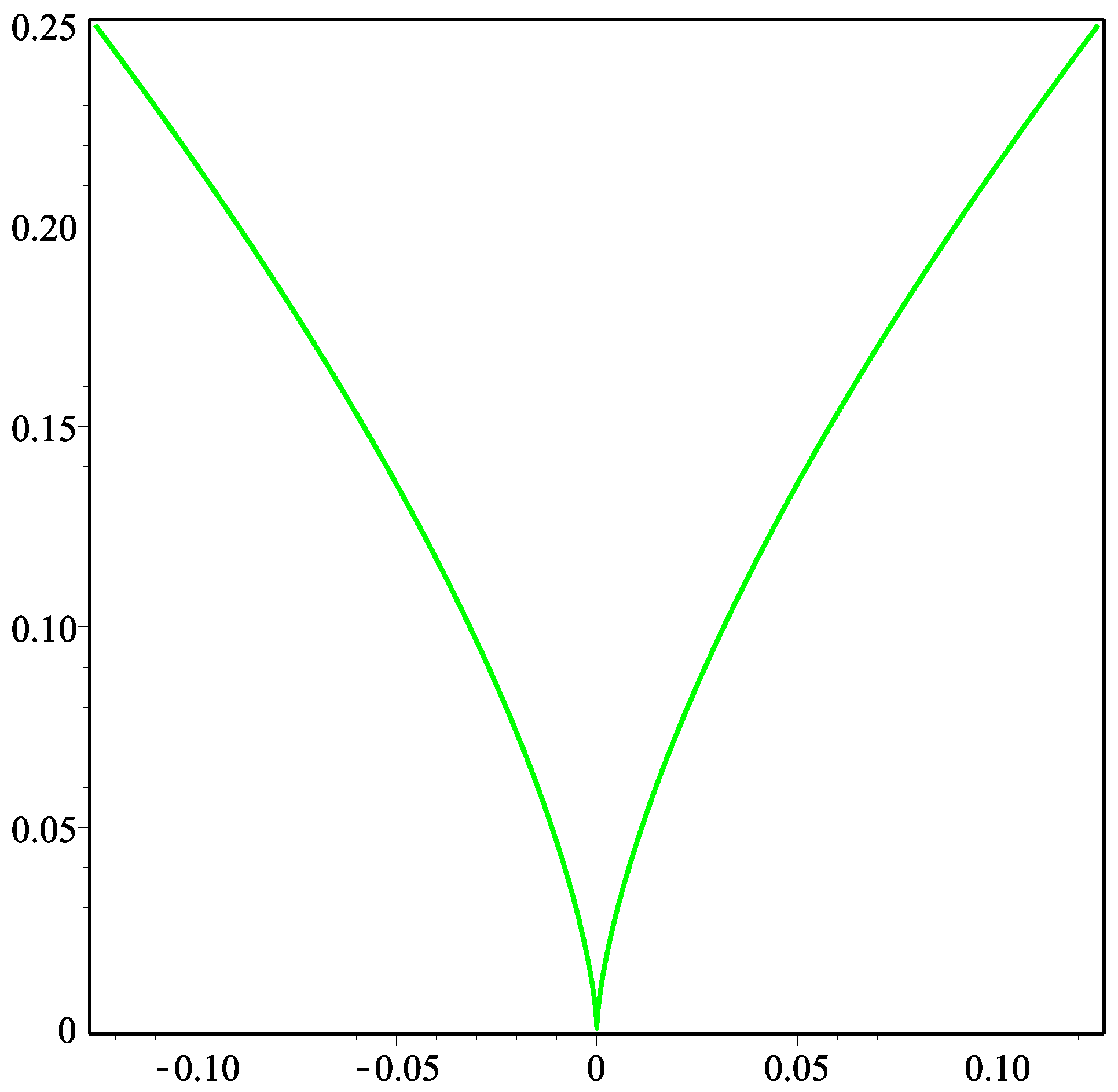
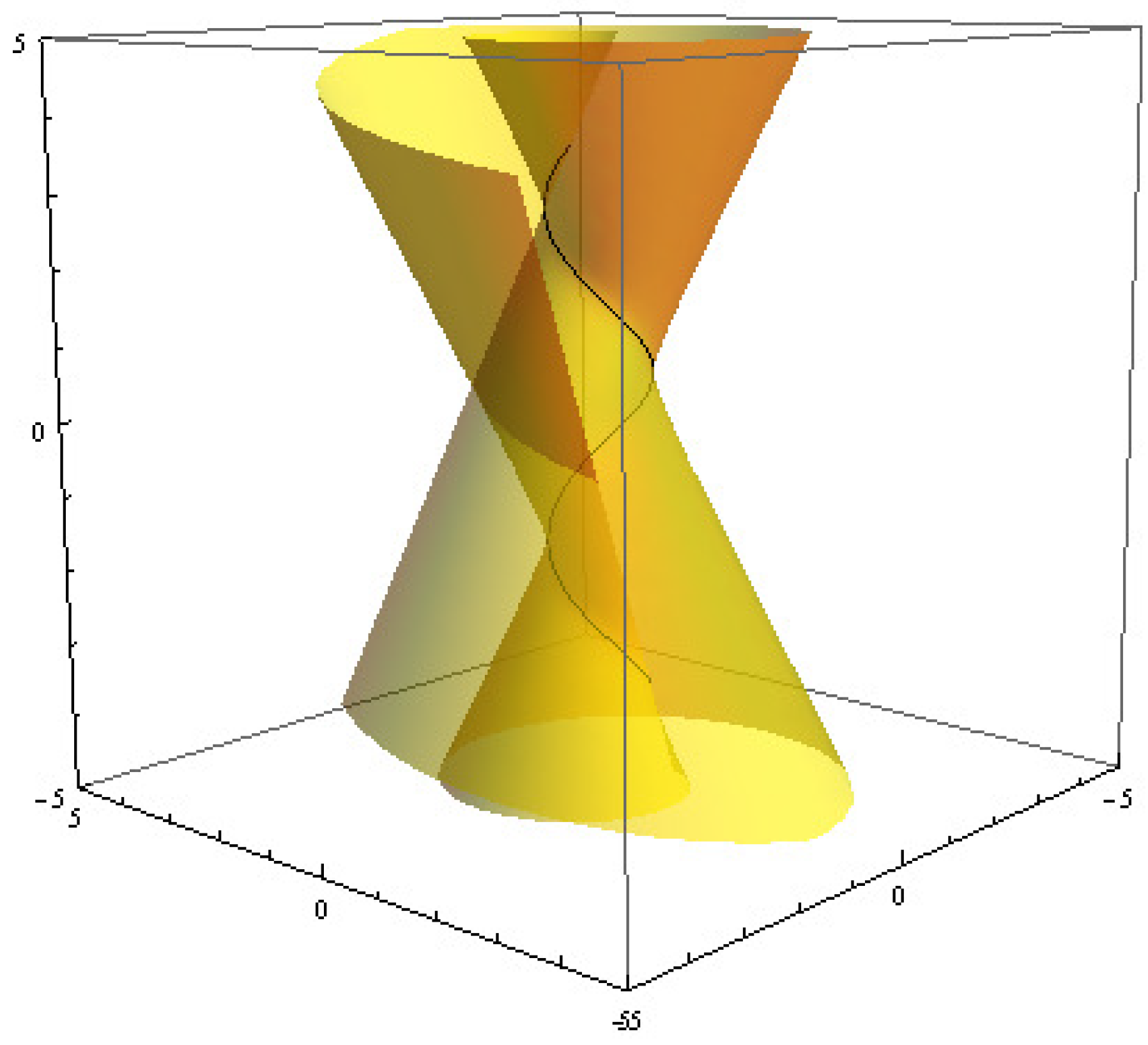
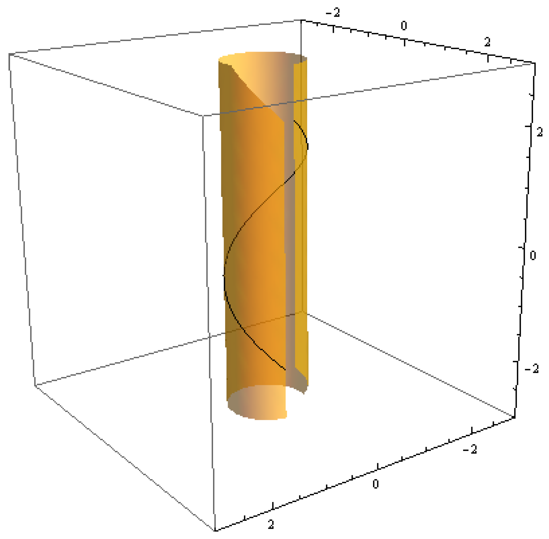
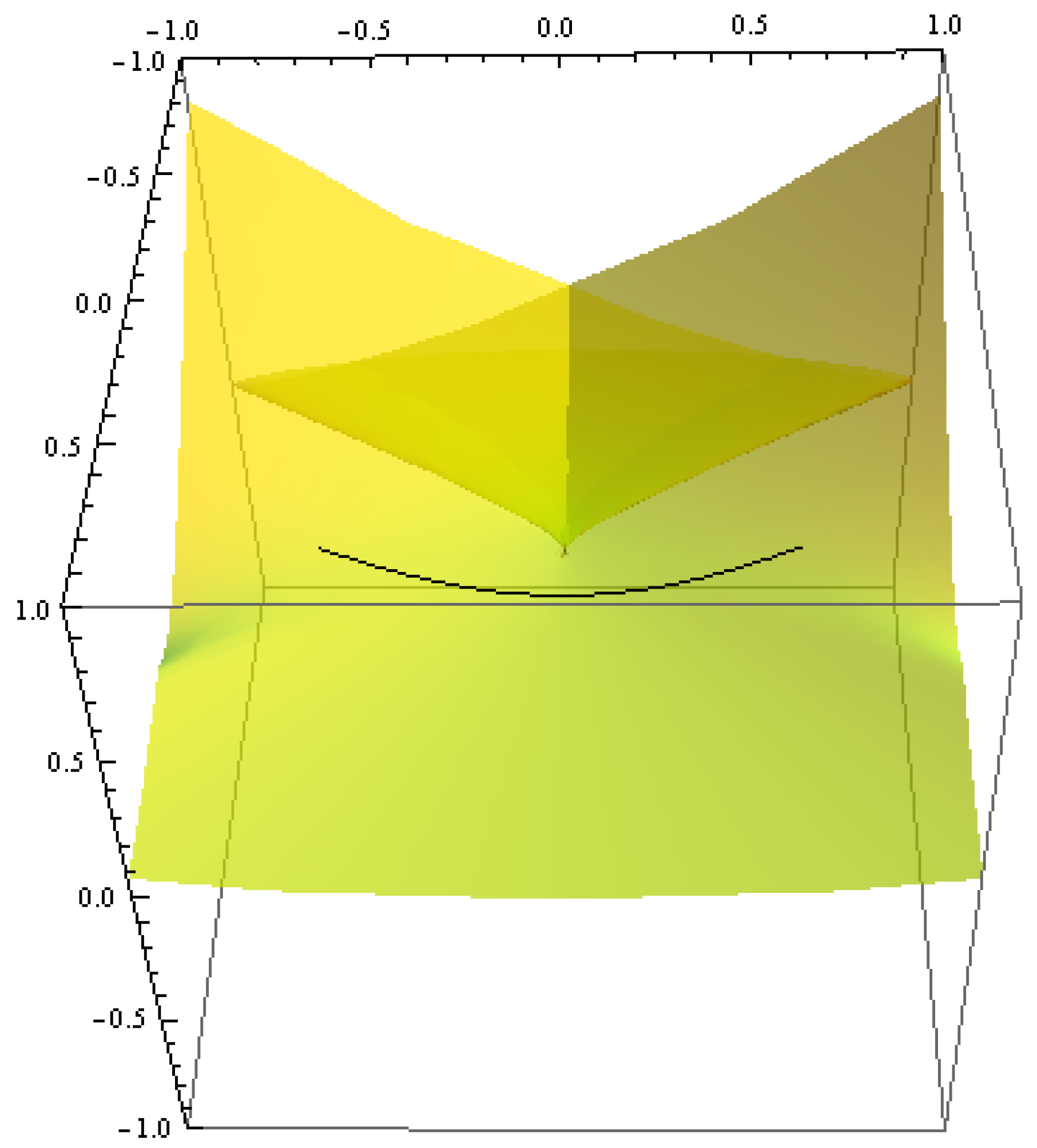
Example 1.
Let γ ( s ) = ( 2 2 sin s , 2 2 cos s , 2 2 s ) , where s is the arc-length parameter. Then
t ( s ) = ( 2 2 cos s , 2 2 sin s , 2 2 ) , n ( s ) = sin s , cos s , 0 , b ( s ) = ( 2 2 cos s , 2 2 sin s , 2 2 ) .
We can calculate that κ ( s ) = 2 2 and τ ( s ) = 2 2 . Therefore, the one-parameter developable surfaces of γ is as follows:
D θ ( s , u ) = γ ( s ) + u t ( s ) sin θ cos θ n ( s ) + cos 2 θ b ( s ) 1 + cos 2 θ .
The tangent developable surface of γ is as follows:
D π 2 ( s , u ) = ( 2 2 sin s 2 2 u cos s , 2 2 u sin s 2 2 cos s , 2 2 s + 2 2 u ) .
In this case, δ ( s ) 2 2 and σ ( s ) 1 . By Theorem 2 (2)-(i), we have the cuspidal edge singularities at u = 0 (Figure 4). The rectifying developable surface of γ is as follows:
D 0 ( s , u ) = ( 2 2 sin s , 2 2 cos s , 2 2 s 2 u ) .
In this case, δ ( s ) 0 . By Theorem 1, the rectifying developable surface of γ is a cylinder (Figure 5).
Example 2.
Let γ ( s ) = ( 1 2 s 2 , 1 4 s 4 , 0 s 1 t 2 t 6 d t ) , where s ( 0.68 , 0.68 ) . Then, we have
t ( s ) = ( s , s 3 , 1 s 2 s 6 ) , n ( s ) = ( 1 s 2 s 6 1 + 9 s 4 4 s 6 , 3 s 2 1 s 2 s 6 1 + 9 s 4 4 s 6 , s ( 1 + 3 s 4 ) 1 + 9 s 4 4 s 6 ) , b ( s ) = ( s 2 ( 3 + 2 s 2 ) 1 + 9 s 4 4 s 6 , 1 + 2 s 6 1 + 9 s 4 4 s 6 , 2 s 3 1 s 2 s 6 1 + 9 s 4 4 s 6 ) .
We can calculate that κ ( s ) = 1 s 2 s 6 1 + 9 s 4 4 s 6 and τ ( s ) = 2 s ( 4 s 8 12 s 6 4 s + 3 ) ( 1 + 9 s 4 4 s 6 ) 1 s 2 s 6 . Therefore, the one-parameter developable surface of γ is as follows:
D θ ( s , u ) = γ ( s ) + u 2 s ( 4 s 8 12 s 6 4 s + 3 ) t ( s ) ( 1 s 2 s 6 ) 1 + 9 s 4 4 s 6 cos θ ( sin θ n ( s ) cos θ b ( s ) ) 4 s 2 ( 4 s 8 12 s 6 4 s + 3 ) 2 + ( 1 s 2 s 6 ) ( 1 + 9 s 4 4 s 6 ) cos 2 θ .
The tangent developable surface of γ is as follows:
D π 2 ( s , u ) = ( 1 2 s 2 + u s , 1 4 s 4 + u s 3 , 0 s 1 t 2 t 6 d t + u 1 s 2 s 6 ) .
In this case, δ ( s ) = 1 + 9 s 4 4 s 6 1 s 2 s 6 0 when s ( 0.68 , 0.68 ) . Since τ 2 ( s ) + κ 2 ( s ) cos 2 θ 0 , then σ ( s ) 1 . By Theorem 2 (2)-(i), we have the cuspidal edge singularities are at u = 0 if s 0 (Figure 6). The rectifying developable surface of γ is as follows:
D 0 ( s , u ) = ( 1 2 s 2 + u 2 s 2 ( 4 s 8 12 s 6 4 s + 3 ) + u s 2 ( 1 s 2 s 6 ) ( 3 + 2 s 2 ) 4 s 2 ( 4 s 8 12 s 6 4 s + 3 ) 2 + ( 1 s 2 s 6 ) ( 1 + 9 s 4 4 s 6 ) , 1 4 s 4 + u 2 s 4 ( 4 s 8 12 s 6 4 s + 3 ) + u ( 1 s 2 s 6 ) ( 1 + 2 s 6 ) 4 s 2 ( 4 s 8 12 s 6 4 s + 3 ) 2 + ( 1 s 2 s 6 ) ( 1 + 9 s 4 4 s 6 ) , 0 s 1 t 2 t 6 d t + u 2 s ( 4 s 8 12 s 6 4 s + 3 ) 1 s 2 s 6 + u 2 s 3 ( 1 s 2 s 6 ) 1 s 2 s 6 4 s 2 ( 4 s 8 12 s 6 4 s + 3 ) 2 + ( 1 s 2 s 6 ) ( 1 + 9 s 4 4 s 6 ) ) .
In this case, we have
δ ( 0 ) = τ ( s ) κ ( s ) | s = 0 = 2 ( 3 12 s 2 73 s 4 + 126 s 6 84 s 8 130 s 10 + 252 s 12 120 s 14 + 32 s 16 + 24 s 18 ) ( 1 s 2 s 6 ) ( 1 + 9 s 4 4 s 6 ) 5 2 | s = 0 = 6
and
σ ( 0 ) = [ s ( 1 + 9 s 4 4 s 6 ) 3 2 ( 3 12 s 2 73 s 4 + 126 s 6 84 s 8 130 s 10 + 252 s 12 120 s 14 + 32 s 16 + 24 s 18 ) 2 ( 9 + 281 s 2 1144 s 4 405 s 6 + 6397 s 8 9474 s 10 + 10 , 962 s 12 10 , 698 s 14 + 6396 s 16 + 1854 s 18 8180 s 20 + 6616 s 22 1728 s 24 + 536 s 26 + 144 s 28 ) ] | s = 0 = 0 .
We can also calculate σ ( 0 ) = 1 . By Theorem 2 (3), we have the swallowtail singularities at ( 0 , 1 6 ) (Figure 7).

Author Contributions

Conceptualization, Q.Z.; Writing—Original Draft Preparation, Q.Z.; Calculations, D.P.; Manuscript Correction, D.P.; Giving the Examples, Y.W.; Drawing the Pictures, Y.W.

Funding

This research was funded by National Natural Science Foundation of China grant numbers 11271063 and 11671070 and the Fundamental Research Funds for the Central Universities grant number 3132018220.

Acknowledgments

This research was funded by National Natural Science Foundation of China grant numbers 11271063 and 11671070 and the Fundamental Research Funds for the Central Universities grant number 3132018220.

Conflicts of Interest

The authors declare no conflict of interest.

References

  1. Ishikawa, G. Topological classification of the tangent developable of space curves. J. Lond. Math. Soc. 2000, 62, 583–598. [Google Scholar] [CrossRef]
  2. Izumiya, S.; Katsumi, H.; Yamasaki, T. The Rectifying Developable and the Spherical Darboux Image of a Space Curve. Banach Center Publ. 1999, 50, 137–149. [Google Scholar] [CrossRef]
  3. Pottmann, H.; Wallner, J. Approximation algorithms for developable surfaces. Comput. Aided Geom. Des. 1999, 16, 539–556. [Google Scholar] [CrossRef] [Green Version]
  4. Solomon, J.; Vouga, E.; Wardetzky, M.; Grinspun, E. Flexible developable surfaces. Comput. Graph. Forum 2012, 31, 1567–1576. [Google Scholar] [CrossRef]
  5. Tang, C.; Bo, P.; Wallner, J.; Pottmann, H. Interactive design of developable surfaces. ACM Trans. Graph. 2016, 35, 1–12. [Google Scholar] [CrossRef]
  6. Cayley, A. On the developable surfaces which arise from two surfaces of second order. Camb. Dublin Math. J. 1850, 2, 46–57. [Google Scholar]
  7. Sun, J.; Pei, D. Singularity analysis of Lorentzian hypersurfaces on pseudo n-spheres. Math. Methods Appl. Sci. 2015, 38, 2561–2573. [Google Scholar] [CrossRef]
  8. Sun, J.; Pei, D. Singularity properties of one-parameter lightlike hypersurfaces in Minkowski 4-space. J. Nonlinear Sci. Appl. 2015, 8, 467–477. [Google Scholar] [CrossRef]
  9. Wang, Y.; Pei, D.; Cui, X. Pseudo-spherical normal Darboux images of curves on a lightlike surface. Math. Methods Appl. Sci. 2017, 40, 7151–7161. [Google Scholar] [CrossRef]
  10. Wang, Y.; Pei, D.; Gao, R. Singularities for one-parameter null hypersurfaces of Anti-de Sitter spacelike curves in semi-Euclidean Space. J. Funct. Spaces 2016, 2, 1–8. [Google Scholar] [CrossRef]
  11. Izumiya, S.; Takeuchi, N. Geometry of ruled surfaces. Appl. Math. Gold. Age 2003, 18, 305–338. [Google Scholar]
  12. Bruce, J.W.; Giblin, P.J. Curves and Singularities; Cambridge Press: Cambridge, UK, 1992. [Google Scholar]
  13. Arnol’d, V.I.; Gusein-Zade, S.M.; Varchenko, A.N. Singularities of Differentiable Maps; Birkhäuser: New York, NY, USA, 1986; Volume I. [Google Scholar]
  14. Damon, J. The Unfolding and Determinacy Theorems for Subgroups of A and K; Memoirs American Mathematical Society: Providence, RI, USA, 1984. [Google Scholar]
  15. Stoker, J.J. Differential Geometry. In Pure and Applied Math; Wiley-Interscience: New York, NY, USA, 1969. [Google Scholar]
Figure 1. Cusp.
Figure 1. Cusp.
Symmetry 11 00108 g001
Figure 2. Cuspidal edge.
Symmetry 11 00108 g002
Figure 3. Swallowtail.
Symmetry 11 00108 g003
Figure 4. γ and D π 2 ( s , u ) of Example 1.
Symmetry 11 00108 g004
Figure 5. γ and D 0 ( s , u ) of Example 1.
Symmetry 11 00108 g005
Figure 6. γ and D π 2 ( s , u ) of Example 2.
Symmetry 11 00108 g006
Figure 7. γ and D 0 ( s , u ) of Example 2.
Symmetry 11 00108 g007

