Article

Noise-Robust Sound-Event Classification System with Texture Analysis

Department of Computer Convergence Software, Korea University, Sejong Campus, Sejong City 30019, Korea
*
Authors to whom correspondence should be addressed.
Symmetry 2018, 10(9), 402; https://doi.org/10.3390/sym10090402
Submission received: 29 August 2018 / Revised: 12 September 2018 / Accepted: 13 September 2018 / Published: 15 September 2018

Abstract

:
Sound-event classification has emerged as an important field of research in recent years. In particular, investigations using sound data are being conducted in various industrial fields. However, sound-event classification tasks have become more difficult and challenging with the increase in noise levels. In this study, we propose a noise-robust system for the classification of sound data. In this method, we first convert one-dimensional sound signals into two-dimensional gray-level images using normalization, and then extract the texture images by means of the dominant neighborhood structure (DNS) technique. Finally, we experimentally validate the noise-robust approach by using four classifiers (convolutional neural network (CNN), support vector machine (SVM), k-nearest neighbors(k-NN), and C4.5). The experimental results showed superior classification performance in noisy conditions compared with other methods. The F1 score exceeds 98.80% in railway data, and 96.57% in livestock data. Besides, the proposed method can be implemented in a cost-efficient manner (for instance, use of a low-cost microphone) while maintaining high level of accuracy in noisy environments. This approach can be used either as a standalone solution or as a supplement to the known methods to obtain a more accurate solution.

1. Introduction

Sound-event classification has seen a noticeable increase in interest as a field of research [1,2,3,4,5,6]. Supported by advancements in information communication technology (ICT) and convergence technology in the Industry 4.0 era [7], various industries are conducting research using sound data. In recent times, numerous studies have been conducted in the livestock industry [8,9,10] and railway industry [11,12,13,14,15], making it a broad research topic under the concepts of Industry 4.0. Detection of pig respiratory diseases using sound-signal analysis has been reported where the convergence of research in the livestock industry and IT can be seen. Early detection of respiratory diseases on a livestock farm is a critical factor in avoiding large economic losses due to the death of livestock [9,10]. For example, a study was conducted by Reference [8] to identify respiratory diseases in pigs by using the dynamic time-warping (DTW) algorithm after generating feature vectors by applying filtering and amplitude-modulation techniques in the sound-frequency band. Furthermore, research in Reference [9] focused on detecting respiratory diseases by using mel-frequency cepstral coefficients (MFCC) sound-feature information and support-vector data description (SVDD). The latter is a one-class classifier that can detect porcine respiratory diseases. Subsequently, a sparse representation classifier (SRC) was used to classify the respiratory diseases. On the other hand, another study described methods to select and combine only the features (among various sound features of the time and frequency domains) that are effective in detecting pig respiratory diseases [10]. Significant work has also been reported pertaining to the railway industry on the detection of faulty parts and determining the replacement time of railway-point machines. A seemingly trivial problem can result in tragic accidents, causing huge economic losses and human fatalities. A few examples of prior research include the following: The work in References [11,12] proposed a monitoring system that keeps track of a railway-point machine’s status using electrical signals (current and voltage). A practical fault-detection system based on a DTW method was also suggested to detect anomalies in railway-point machines, which could be applied directly to real-world railway sites without requiring a learning process [13]. A study on an aging-condition detection system using electrical signals and applying the SVDD method was also introduced in Reference [14]. In addition to that, a detection and classification system for railway-point machines using MFCC feature information that has been extracted from the sound signals was recently presented by Reference [15].
While previous studies on livestock and railway industries showed promising results, one cannot guarantee that the influence of the noise generated in the physical environment was sufficiently taken into consideration. Generally, sound-event classification tasks become more difficult with the increase in noise levels. Many traditional methods show weak performance in the presence of ambient noise [6]. This study focuses on handling the problem of noise, which can significantly affect the classification of sound events. To demonstrate the effectiveness of an academic prototype, noise robustness that can be immune from real-world noise sources must be ensured. A noise-robust algorithm is one of the major research topics in the field of signal analysis. For example, a feature vector combining modulation-feature information extracted from the spectrogram of a sound signal and the MFCC, which showed noise-robust performance, was presented in Reference [16]. Among various methods, the dominant neighborhood structure (DNS) algorithm [17] is of high interest. This method aims to solve the problem of image noise by converting it into a texture image.
In this study, we evaluate recent developments on the noise problem, and propose a noise-robust sound-event classification system that can be applied in noisy real-world environments. The proposed method applies the DNS algorithm by extracting the texture image to solve the problem of a sound signal that has structural weakness in noisy environments. This method is verified using data from the railway industry and the livestock industry. Experiments were conducted using various classifiers to verify the noise robustness of DNS. These experiments show that the proposed method can accurately classify sound events with stability while ensuring robustness in the presence of noise. To the best of our knowledge, this is the first report on using the texture information of sound signals for classifying sound events in noisy environments.
The remainder of this paper is structured as follows. In Section 2, we describe the proposed method using texture analysis to classify sound events in noisy environments. In Section 3, we analyze the performance and experimental results. In Section 4, we draw conclusions and provide directions for future work.

2. Classification of Sound Events Using Noise-Robust Systems

Figure 1 shows the overall structure of the noise-robust sound-event classification system that applies texture analysis using DNS. The system consists of a preprocessing module, a texture-extract module, and a classification module.

2.1. Preprocessing Module

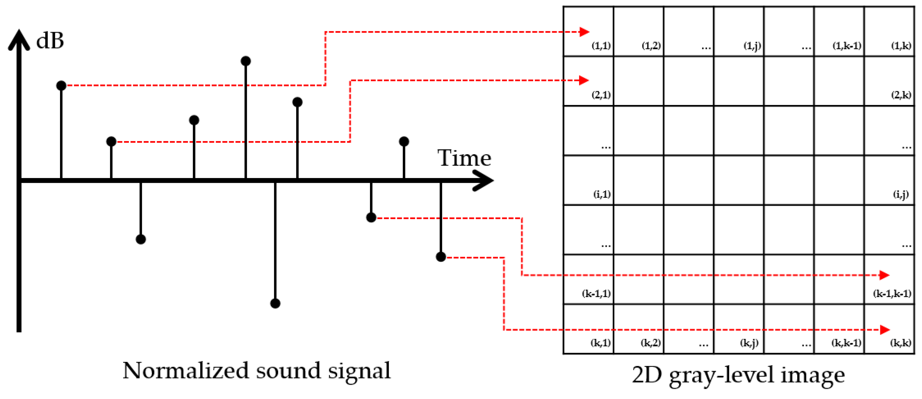
In the preprocessing module, the sound signal is converted into a two-dimensional grayscale image. First, the length of the sound signal is normalized by linear transformation while maintaining the inherent traits of the sound signal. Since the dataset consists of temporally trimmed sound data of different lengths (varying between 4.5 s and 5.7 s for the railway data, and between 0.13 s and 2.66 s for the pig data), we applied linear transformation to each piece of data as a whole, without using a sliding time window to generate normalized sound signals of the same length. Then, normalized data go through one more normalization process. In the data-conversion process to obtain a two-dimensional gray-level image, the value of each sample of the sound signal is normalized between 0 and 255. The normalized value of each sample corresponds to the pixel value of the two-dimensional gray-level image, as shown in Figure 2. In this process, the normalized sound signal on the left side of Figure 2 is vertically mapped to the right side of the two-dimensional gray-level image of size k × k. We compared the portrait priority to the landscape priority. We concluded that whether portrait or landscape is selected, performance was not affected. The only difference between the two was the direction of the texture.

2.2. Texture-Extract Module

In the texture-extract module, texture information is extracted from the two-dimensional gray-level image using the DNS algorithm proposed in Reference [17]. The DNS method has already been proven to be robust in the image-processing field, where noise commonly exists [18]. In this study, we aim to extend the application to sound signals. Figure 3 shows the overall process of extracting a texture image using the DNS algorithm, which can be summarized as follows. To generate a texture image, the searching window and the neighborhood window must be defined first. The fixed pixel is located at the center of the searching window, and the other pixels in the searching window are defined as neighboring pixels. The algorithm sets a searching window of size n × n for the texture image size to be extracted, and generates a vector V s . by setting a neighborhood window of size m by m around the fixed pixel in the searching window. Next, vector V n is generated by setting the neighborhood window of size m by m around the pixel located at the upper-left corner of the searching window. After this operation, the Euclidean distance is calculated between V s and V n , and the pixel value of the texture image is sequentially calculated from the upper-left corner to the bottom-right corner from the searching window. This process is repeated until all the pixels in the searching window are computed and the final texture image is generated. The final texture image of m × m has the same dimensions as the searching window that was set initially.

2.3. Classification Module

In the classification module, various classifiers are used to prove the robustness (to noise) of the texture image developed by the DNS algorithm. This module is based on deep-learning and machine-learning techniques. The following is a general description of the different classifiers.
  • Convolutional neural networks (CNN): CNN is a representative deep-learning model for image classification [19]. It consists of a convolution layer, a pooling layer, and a fully connected layer [20]. The convolution layer extracts a feature map through a convolution operation on the input image. Based on the features extracted from the convolution layer, the pooling layer applies a subsampling method (max, min, average pooling, etc.) and abstracts the input space to reduce weak features and extract strong features. The fully connected layer is used for the purpose of object classification using the features extracted through iteration between the convolution layer and the pooling layer. From the last layer to the initial layer, a back-propagation algorithm is used to optimize learning by finding weights that minimize error. This gradually extracts the strong-feature maps and develops high-accuracy models through continuous iterative learning. In this study, the CNN structure was designed as shown in Figure 4. The same layer structure was later used for both data types studied in this work (railway industry and livestock industry).
  • Support vector machine (SVM): SVM is widely used in binary classification problems. This is a method of classification by finding an optimal linear-decision plane based on the concept of minimizing structural risk [21,22]. The decision plane is a weighted combination of learning elements called support vectors that exist at the interfaces between the classes. For example, assume that we are analyzing a dataset that can be linearly separated. The goal is to separate the classes by a hyperplane that maximizes the distance of the support vectors. This hyperplane is called an optimal separating hyperplane, and it obtains a support vector by solving a quadratic programming problem. In the case of data that cannot be linearly separated, the input vector is nonlinearly mapped to a higher-dimensional feature space where the linear hyperplane is found. At this time, the objective function and the decision function are calculated as the inner product of the vector. It is not necessary to explicitly calculate the mapping process of the complex calculation. That is, a kernel function satisfying the Mercer condition can be replaced with a mapping function that is used in place of a data vector. In this study, we used the radial basis function (RBF) as a kernel function.
  • k-nearest neighbors algorithm (k-NN): k-NN is representative nonparametric methodology. This is a machine-learning algorithm applied to data classification [23]. As the name implies, k-NN determines the class of data by referring them to the k-closest data points. The Euclidean distance method is usually used to measure the distance.
  • C4.5: The C4.5 algorithm [24] is a tree-based classification algorithm that is an improvement over the ID3 algorithm. Since ID3 is a decision-tree algorithm, analysts can easily understand and explain its results. However, unlike other probabilistic classification algorithms, it is impossible to make predictions when using this method, and only classifying data is allowed. In order to overcome the shortcomings of the ID3 algorithm, the C4.5 algorithm considers more properties, such as, “handling of numerical attributes”, “problem excluding nonsignificant properties”, “tree-depth problem”, “missing-value processing”, and “cost consideration.”

3. Experimental Results

To evaluate the proposed method, we used two sets of data from two different industries. The first set of experiments was conducted on the railway industry, while the livestock industry was used for the second set of experiments. To measure robustness to noise, the structural similarity (SSIM) method was used to quantitatively analyze the texture of the images extracted by DNS. The SSIM method measures the similarity between the original image and the distortions caused by compression and transformation. It assumes that the loss of image quality occurs due to the structural distortion of the image signal itself [25]. SSIM is expressed as a numerical value between 0 and 1, where a value close to 1 implies that the difference in image quality between the original image and the comparative image is small. Finally, the validity of the proposed method is demonstrated experimentally by using four classifiers (CNN, SVM, k-NN, and C4.5). All classifiers were trained with noise-free data, and then tested using a combination of white Gaussian noise and environmental noise that can occur in real-life situations in both industries.

3.1. Experimental Results on Railway-Point-Machine Sound Data

3.1.1. Experimental Data

In this experiment, a sound sensor (SHURE SM137) was placed in front of a railway-point machine to collect the sound generated whenever a railway-point machine switched. Sound data were collected from a railway-point machine of type NS-AM in the Sehwa Company located in Daejeon, South Korea, on 1 January 2016 [15]. The waveforms and spectrograms of the sound signals were manually edited for their use in the experiments. Each piece of sound data was 4.5 to 5.7 s long. The sound dataset used in the experiments consisted of 150 data under normal conditions, and 438 data under abnormal conditions (142 for gravel condition, 141 for ice-covered condition, and 155 for unscrewed condition). In addition, white Gaussian noise (signal-to-noise ratio (SNR): 18, 15, 12, 9, 6, 3, and 0 dB) and environmental noise (i.e., noises from birds, wind, rain, and passing helicopters and trains) were added to the collected sound signals to create a test dataset for use in the experiments. The basic statistics for the collected environmental noise are shown in Table 1, where the smaller the SNR value was, the stronger the noise. Figure 5 shows the sound waveforms acquired from the railway-point machine for each event. Noticeably, the sound signal of each event is difficult to distinguish with the naked eye.

3.1.2. Extracting Texture Image and Analysis

The texture image was extracted by applying DNS to the two-dimensional gray-level image created by the preprocessing module. In the DNS experiment, the size of the searching window was 64 × 64, and the size of the neighborhood window was 32 × 32. As a result, a 64 × 64 texture image was generated. The average execution time required to generate the texture image using the DNS algorithm was 0.4621 s. Total execution time was 0.4491 to 0.5520 s depending on the length of the sound event. Standard deviation was 0.0106. Results show that the time required to get results with this method is short enough for it to be used in real time for actual railways even if the length of the event time is about 4.5 to 5.7 s.
Figure 6 shows the texture images extracted from the sound events in a railway-point machine. We can clearly see that the sound waveforms, which were difficult to distinguish in Figure 5, have their own texture information in Figure 6. Figure 6a shows the texture information of diagonal lines extending form the upper-left corner to the lower-right corner, representing a normal event. This texture information is divided into three horizontal partitions. Figure 6b shows a gravel event, which has very strong horizontal texture information divided into three parts. Figure 6c is for an ice-covered event, with weak diagonal texture information that extends from the upper-right corner to the lower-left corner. Texture information is divided into three horizontal partitions. Figure 6d shows an unscrewed event, with texture information similar to the normal event, but noticeably weaker.
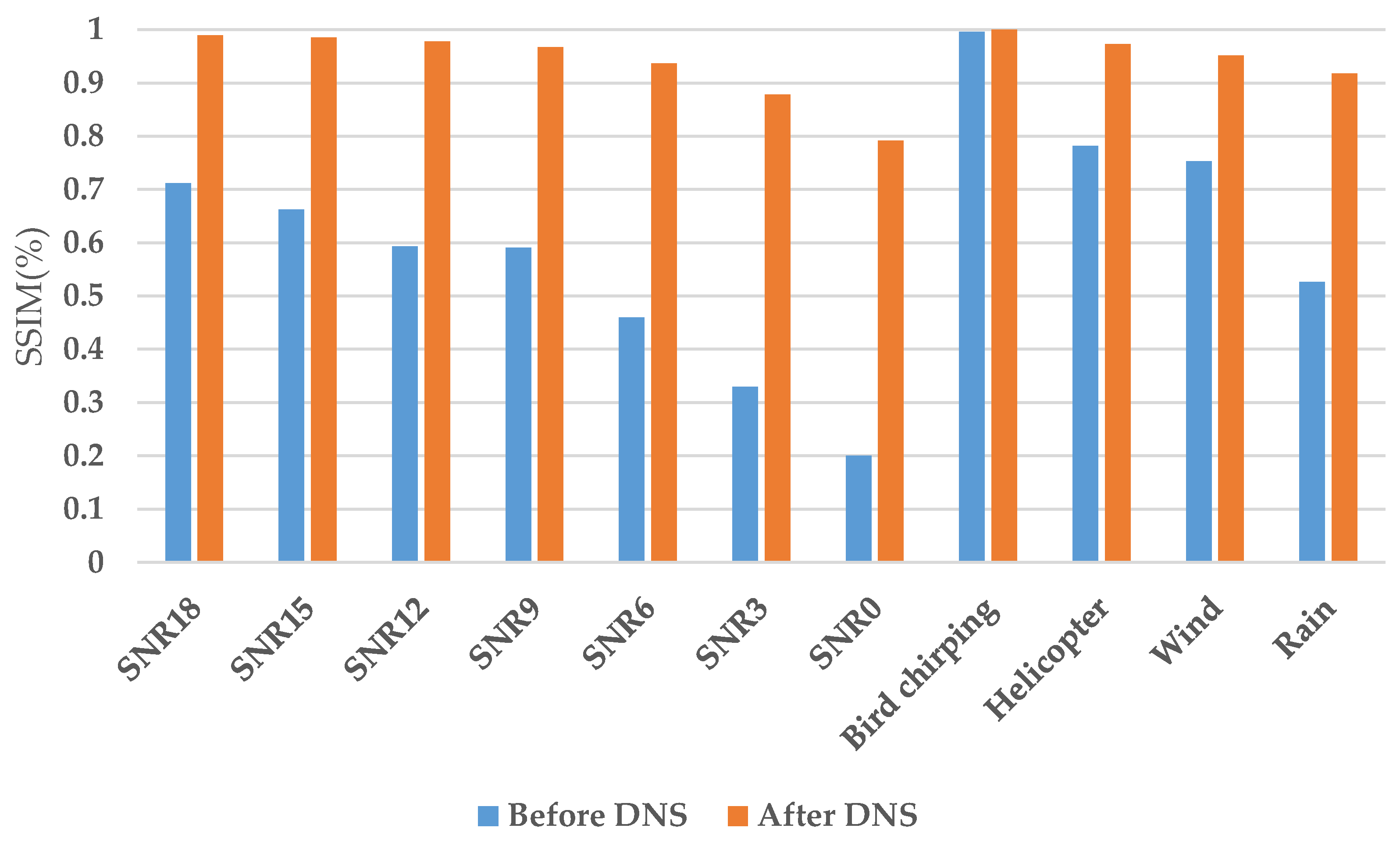
To verify the proposed method’s robustness against noise, we added white Gaussian noise and various environmental noises to a normal sound event. Figure 7 shows some examples of the process of transforming sound signals into texture images. As seen in Figure 7 (sequentially compared according to the SNR), most of the white Gaussian noise and the environmental noise was removed with the DNS algorithm. It can be visually confirmed that the unique texture information was constantly maintained. We used SSIM to quantify the degree of noise removal (see Figure 8). The blue line in the graph in Figure 8 is the SSIM value before applying DNS, and the orange line is the SSIM similarity value after applying DNS.

3.1.3. Classification Results

In this experiment, four classifiers (CNN, SVM, k-NN, and C4.5) were used to verify the robustness of DNS against noise. CNN was designed with Keras 2.1.5 API (https://keras.io) using TensorFlow 1.21 (https://www.tensorflow.org) as a backend. Parameter options used for the CNN learning process were: Xavier initialization function, Adam optimizer with a learning rate of 0.001, decay rates β 1 = 0.9 and β 2 = 0.999, ReLU activation function, and a dropout ratio of 30% (activate 70%) in hidden layers and 50% in fully connected layers. We set the training epochs to 4000 epochs and performed early stopping after 50 epochs of no improvement in the training process. We used the default parameters for the other classifiers. All classifiers were trained with noise-free data and tested with data containing various environmental noises.
The performance of the proposed method was evaluated by precision, recall, and F1 score. Precision is the ratio of positive detection to the detected results. Recall is the ratio of data successfully detected in the input data [26,27]. F1 score is calculated as the harmonic mean of the precision and recall considering the tradeoff between them. The equations are as follows [28]:
Precision = T P T P + F P × 100
Recall = T P T P + F N × 100
F 1   score = 2 × precision × recall precision + recall
where True Positive (TP) are the data correctly identified as true data, False Positive (FP) are the data incorrectly identified as true data, and False Negative (FN) are the data incorrectly identified as false data.
A summary of the classification results is shown in Table 2. According to experimental results, most of the white Gaussian noise and the environmental noise have good classification performance in four classifiers as a multiclass classifier, in general. Among them, CNN (the deep-learning model) had the best performance. SNR 0, known as a relatively strong noise, and rain noise, which is a strong environmental noise, also show high classification performance. In the following comparison results, unless explicitly illustrated, we used CNN as a default classifier in order to easily reproduce and compare the performance with other methods.
As indicated in Table 3, classification performance of the proposed method is best when compared with other conventional classification methods. The results show that, when modulation and MFCC methods are used together, as shown in Reference [16], performance improves in the case of environmental noise. However, it yields poor results with white Gaussian noise, and classification performance remains lower than that of the proposed method. Therefore, we experimentally confirmed that the texture information extracted with the DNS algorithm, as proposed in this study, shows robust performance with both white Gaussian noise and environmental noise.

3.2. Experimental Results on Porcine Respiratory Sound Data

3.2.1. Experimental Data

The data used in the second experiment were collected from a total of 36 pigs (Yorkshire, Landrace, and Duroc) with an average weight ranging from 25 to 30 kg in four pigsties in Chungnam, South Korea. The pigs were housed in a 1.8 × 4.8 m pen at a room temperature of about 23 °C. Blood samples were collected from pigs suspected of being infected and subjected to serological analysis to determine postweaning multisystemic wasting syndrome (PMWS), porcine reproductive and respiratory syndrome (PRRS), and mycoplasma hyopneumoniae (MH) infections. Sounds related to the respiratory disease were recorded with a digital camcorder (JVC GR-DVL520A, Yokohama, Japan) at a distance of 1 m from each pig [9]. After editing, the recordings of the respiratory disease events were 0.13 to 2.66 s long. These were of a monotype with a sampling rate of 44,100 Hz. In addition, white Gaussian noise (SNR: 18, 15, 12, 9, 6, 3, and 0 dB) and environmental noise (footsteps, radio operation, and door opening) were added to the collected sound events to create a test dataset. Among the environmental noises, the footsteps of the pigs were collected by dividing the sounds of one or two pigs moving (weak footsteps), and the sounds of several pigs moving (strong footsteps). In addition, the sound from a radio for the psychological stabilization of pigs, and the sound of a door opening when the pig handler entered the pigsty to feed or clean were also collected. Table 4 shows the basic statistics for the collected environmental noise. Figure 9 shows the sound waveforms acquired from the pigsty for each event.

3.2.2. Extracting Texture Image and Analysis

In the experiment, the size of the searching window was 64 × 64 and the size of the neighborhood window was 32 × 32. As a result, a 64 × 64 texture image was generated. The average execution time required to generate the texture image using the DNS algorithm was 0.0979 s, making the total execution time between 0.0905 and 0.1349 s, depending on the length of the sound event. The standard deviation was 0.0063.
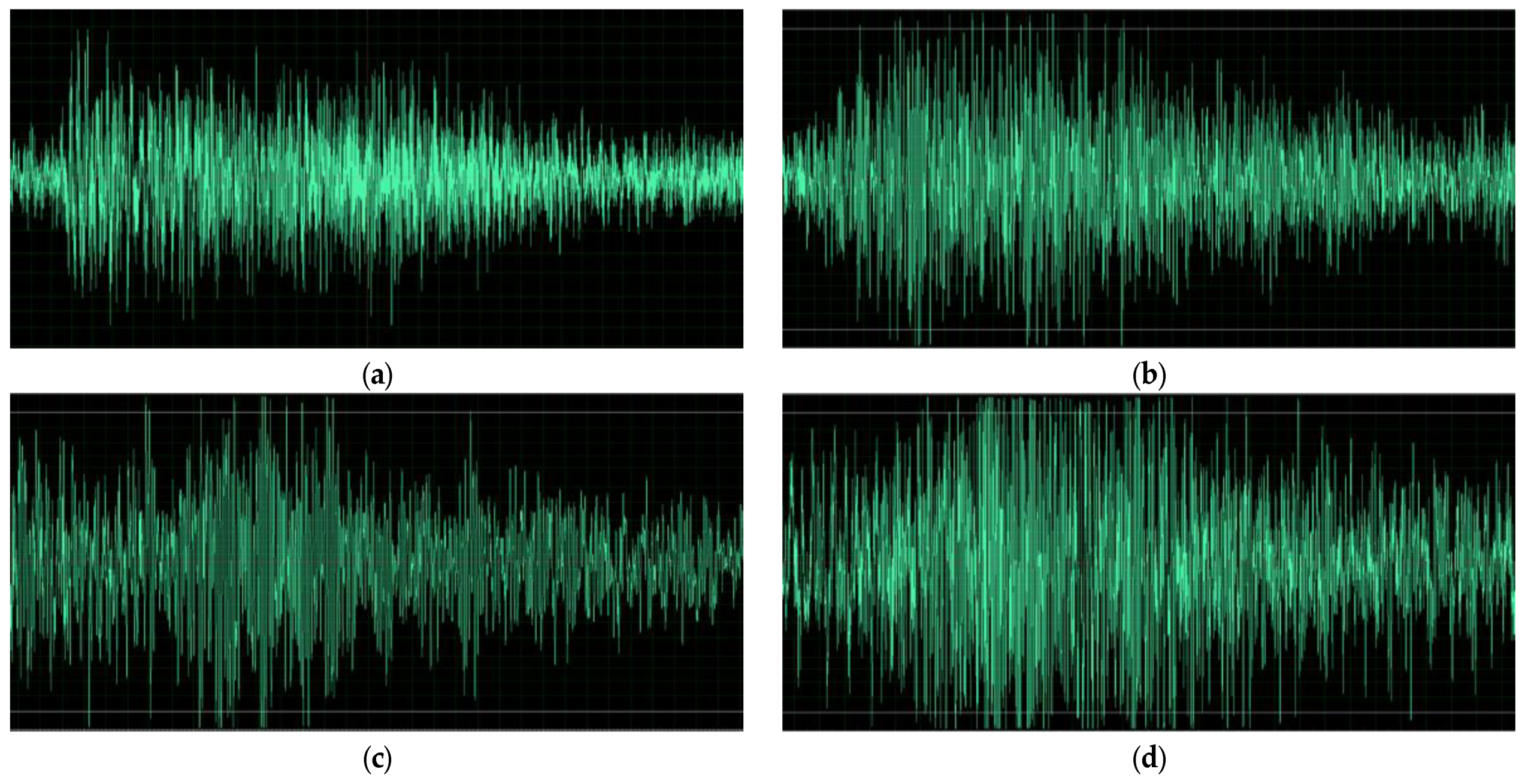
Figure 10 shows the texture images extracted from the sound events in the pigsty. It was confirmed that the sound waveforms, which were difficult to distinguish in Figure 9, have their own texture information in Figure 10. Figure 10a shows a texture that extends horizontally with respect to the center of the image in a normal (grunt) event. Figure 10b shows a texture that is dense and arranged horizontally. Figure 10c shows a horizontal texture based on the center coordinates, and Figure 10d shows a unique diagonal texture.
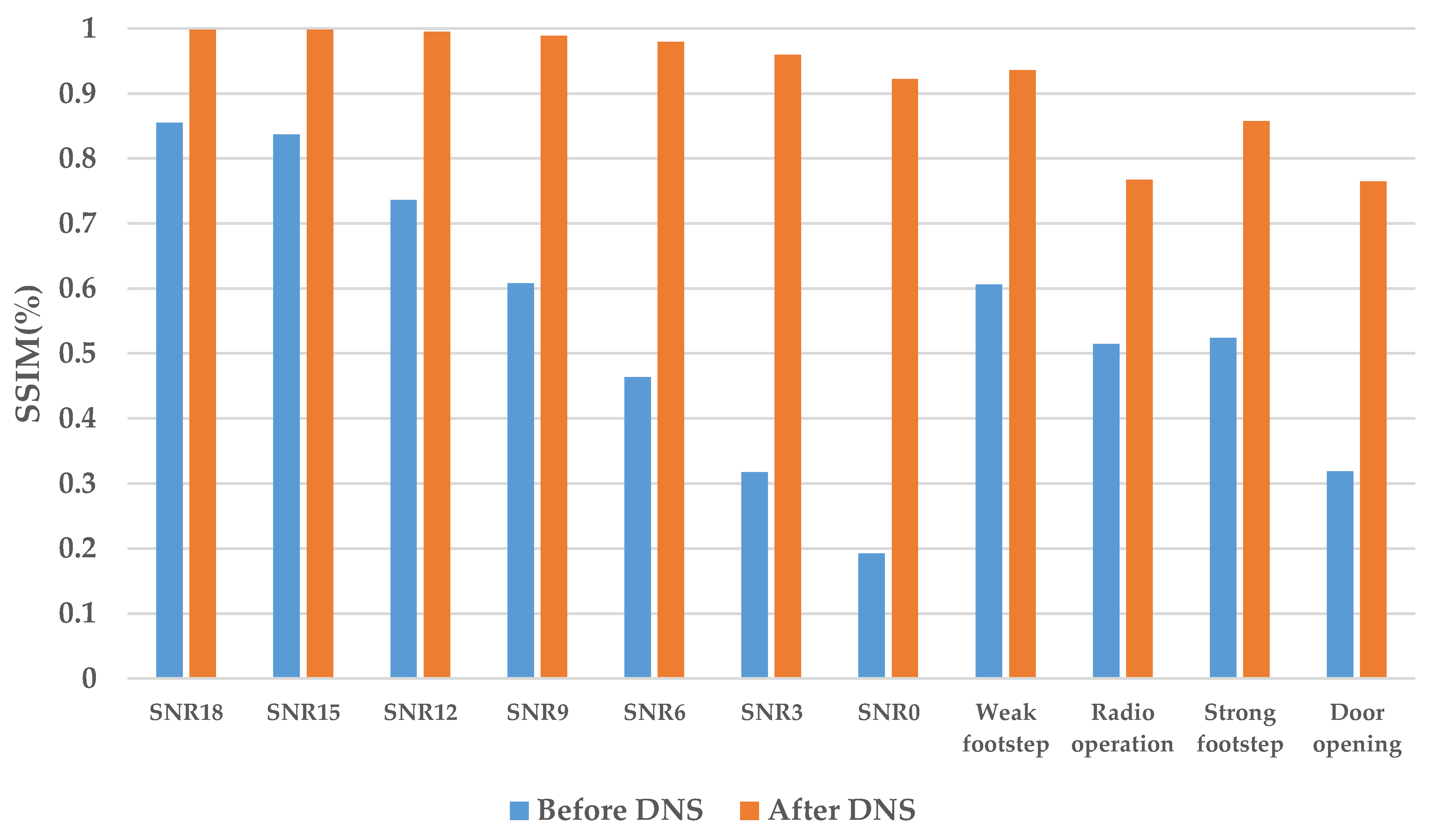
To verify the robustness against the noise, we added white Gaussian noise and environmental noise to a normal (grunt) sound event. The extracted texture image is shown in Figure 11. In Figure 11 (sequentially compared according to the SNR), it can be seen that most of the white Gaussian noise and the environmental noise were removed with the DNS algorithm. One can visually confirm that the unique texture information was constantly maintained. Figure 12 shows the results of using SSIM to identify the quantitative values. The blue line in Figure 12 is the SSIM value before applying DNS, and the orange line is the SSIM similarity value after applying DNS.

3.2.3. Classification Results

To maintain the consistency of the experiments for the proposed method, we kept the same parameters used in the classifiers in the previous experiments (Section 3.1.3). Experimental results are shown in Table 5. Similar to previous results using the railway-point-machine data, classification performance was found to be satisfactory for all classifiers. Similar to the previous case, CNN showed the best performance.
Comparative results are summarized in Table 6. Although conventional methods showed good classification performance over a certain level in noisy conditions, they were still inferior to the proposed method. It was experimentally confirmed that the texture information extracted with the DNS algorithm, as proposed in this study, showed robust performance under both white Gaussian noise and environmental noise conditions.

4. Conclusions

Sound data from the railway industry and the livestock industry were previously used for the purposes of classification of sound events by signal analysis. Even though the feasibility of such applications was demonstrated, those methods were not sufficiently reliable, as the impact of noise from the surrounding environment was not considered. In this study, we proposed a sound-event classification system that shows superior performance in noisy environments. The proposed method normalizes the sound data and extracts texture images using DNS. This proved to be robust against noise. The proposed method was experimentally validated using four different classifiers (CNN, SVM, k-NN, and C4.5), with CNN outperforming the other classifiers. Experimental results showed superior classification performance under noisy conditions for both industrial applications (railway and livestock). In our experiments, 98.80% classification performance was obtained for the railway industry. For the livestock industry, it was 96.57%. Our experiments showed that the proposed method can be used to classify sound events in a cost-efficient manner (for instance, by using a low-cost microphone) while maintaining high levels of accuracy even in the presence of environmental noise. This can be used either as a standalone solution or to complement other known methods to obtain a more accurate solution. In the future, further verification is required with various kinds of datasets to prove the generality of the proposed method. In addition, we are considering a broader test program, applying the proposed method to commercial production conditions, and we plan to conduct multimodal-based convergence research using video signals as well as sound signals to implement a complete real-time system.

Author Contributions

J.L., D.P. and Y.C. (Yongwha Chung) conceived and designed the overall structure of the proposed method; Y.C. (Yongju Choi) and J.L. collected the sound data; Y.C. (Yongju Choi) and O.A. implemented the proposed method and analyzed the experimental results; Y.C. (Yongju Choi), O.A., J.L., D.P. and Y.C. (Yongwha Chung) wrote the paper.

Funding

This research received no external funding.

Acknowledgments

This study was supported by a Korea University Grant.

Conflicts of Interest

The authors declare no conflict of interest.

References

  1. Ozer, I.; Ozer, Z.; Findik, O. Noise Robust Sound Event Classification with Convolutional Neural Network. Neurocomputing 2018, 272, 505–512. [Google Scholar] [CrossRef]
  2. Sharan, R.V.; Moir, T.J. Robust Acoustic Event Classification Using Deep Neural Networks. Inf. Sci. 2017, 396, 24–32. [Google Scholar] [CrossRef]
  3. Adavanne, S.; Pertilä, P.; Virtanen, T. Sound Event Detection Using Spatial Features and Convolutional Recurrent Neural Network. In Proceedings of the IEEE International Conference on Acoustics, Speech and Signal Processing (ICASSP), New Orleans, LA, USA, 5–9 March 2017. [Google Scholar]
  4. Salamon, J.; Bello, J.P. Deep Convolutional Neural Networks and Data Augmentation for Environmental Sound Classification. IEEE Signal Process. Lett. 2017, 24, 279–283. [Google Scholar] [CrossRef]
  5. McLoughlin, I.; Zhang, H.; Xie, Z.; Song, Y.; Xiao, W. Robust Sound Event Classification Using Deep Neural Networks. IEEE/ACM Trans. Audio Speech Lang. Process. 2015, 23, 540–552. [Google Scholar] [CrossRef] [Green Version]
  6. Zhang, H.; McLoughlin, I.; Song, Y. Robust Sound Event Recognition Using Convolutional Neural Networks. In Proceedings of the IEEE International Conference on Acoustics, Speech and Signal Processing (ICASSP), Brisbane, QLD, Australia, 19–24 April 2015. [Google Scholar]
  7. Gilchrist, A. Introducing Industry 4.0; Apress: New York, NY, USA, 2016; pp. 195–215. [Google Scholar]
  8. Guarino, M.; Jans, P.; Costa, A.; Aerts, J.M.; Berckmans, D. Field Test of Algorithm for Automatic Cough Detection in Pig Houses. Comput. Electron. Agric. 2008, 62, 22–28. [Google Scholar] [CrossRef]
  9. Chung, Y.; Oh, S.; Lee, J.; Park, D.; Chang, H.; Kim, S. Automatic Detection and Recognition of Pig Wasting Diseases Using Sound Data in Audio Surveillance. Sensors 2013, 13, 12929–12942. [Google Scholar] [CrossRef] [PubMed]
  10. Lee, J.; Jin, L.; Park, D.; Chung, Y.; Chang, H. Acoustic Features for Pig Wasting Disease Detection. Int. J. Inf. Process. Manag. 2015, 6, 37–46. [Google Scholar]
  11. Asada, T.; Roberts, C.; Koseki, T. An Algorithm for Improved Performance of Railway Condition Monitoring Equipment: Alternating-current point machine case study. Transp. Res. C Emerg. Technol. 2013, 30, 81–92. [Google Scholar] [CrossRef]
  12. Asada, T.; Roberts, C. Development of an Effective Condition Monitoring System for AC Point Machines. In Proceedings of the 5th IET Conference on Railway Condition Monitoring and Non-Destructive Testing (RCM 2011), Derby, UK, 29–30 November 2011. [Google Scholar]
  13. Kim, H.; Sa, J.; Chung, Y.; Park, D.; Yoon, S. Fault Diagnosis of Railway Point Machines Using Dynamic Time Warping. Electron. Lett. 2016, 52, 818–819. [Google Scholar] [CrossRef]
  14. Sa, J.; Choi, Y.; Chung, Y.; Lee, J.; Park, D. Aging Detection of Electrical Point Machines Based on Support Vector Data Description. Symmetry 2017, 9, 290. [Google Scholar] [CrossRef]
  15. Lee, J.; Choi, H.; Park, D.; Chung, Y.; Kim, H.Y.; Yoon, S. Fault Detection and Diagnosis of Railway Point Machines by Sound Analysis. Sensors 2016, 16, 549. [Google Scholar] [CrossRef] [PubMed]
  16. Sharan, R.V.; Moir, T.J. Noise Robust Audio Surveillance Using Reduced Spectrogram Image Feature and One-against-all SVM. Neurocomputing 2015, 158, 90–99. [Google Scholar] [CrossRef]
  17. Khellah, F. Texture Classification Using Dominant Neighborhood Structure. IEEE Trans. Image Process. 2011, 21, 3270–3279. [Google Scholar] [CrossRef] [PubMed]
  18. Khellah, F. Textured Image Denoising Using Dominant Neighborhood Structure. Arab. J. Sci. Eng. 2014, 39, 3759–3770. [Google Scholar] [CrossRef]
  19. Krizhevsky, A.; Sutskever, I.; Hinton, G.E. ImageNet Classification with Deep Convolutional Neural Networks. In Proceedings of the 25th International Conference on Neural Information Processing Systems, Lake Tahoe, NV, USA, 3–6 December 2012; pp. 1097–1105. [Google Scholar]
  20. Cunningham, R.; Sánchez, M.B.; May, G.; Loram, I. Estimating Full Regional Skeletal Muscle Fibre Orientation from B-Mode Ultrasound Images Using Convolutional, Residual, and Deconvolutional Neural Networks. J. Imaging 2018, 4, 29. [Google Scholar] [CrossRef]
  21. Lee, J.; Noh, B.; Jang, S.; Park, D.; Chung, Y.; Chang, H. Stress Detection and Classification of Laying Hens by Sound Analysis. Asian Australas. J. Anim. Sci. 2015, 28, 592–598. [Google Scholar] [CrossRef] [PubMed] [Green Version]
  22. Santos, P.; Villa, L.F.; Reñones, A.; Bustillo, A.; Maudes, J. An SVM-based Solution for Fault Detection in Wind Turbines. Sensors 2015, 15, 5627–5648. [Google Scholar] [CrossRef] [PubMed] [Green Version]
  23. Akbulut, Y.; Sengur, A.; Guo, Y.; Smarandache, F. NS-k-NN: Neutrosophic Set-Based k-Nearest Neighbors Classifier. Symmetry 2017, 9, 179. [Google Scholar] [CrossRef]
  24. Szarvas, G.; Farkas, R.; Kocsor, A. A Multilingual Named Entity Recognition System Using Boosting and C4.5 Decision Tree Learning Algorithms. In International Conference on Discovery Science; Springer: Berlin/Heidelberg, Germany, 2006. [Google Scholar]
  25. Wang, Z.; Bovik, A.C.; Sheikh, H.R.; Simoncelli, E.P. Image Quality Assessment: from Error Visibility to Structural Similarity. IEEE Trans. Image Process. 2004, 13, 600–612. [Google Scholar] [CrossRef] [PubMed]
  26. Han, J.; Kamber, M.; Pei, J. Data Mining: Concepts and Techniques, 3rd ed.; Morgan Kaufman: San Francisco, CA, USA, 2012. [Google Scholar]
  27. Theodoridis, S.; Koutroumbas, K. Pattern Recognition, 4th ed.; Academic Press: Kidlington, Oxford, UK, 2009. [Google Scholar]
  28. Powers, D.M.W. Evaluation: From Precision, Recall and F-Factor to ROC, Informedness, Markedness and Correlation. J. Mach. Learn. Technol. 2011, 2, 2229–3981. [Google Scholar]
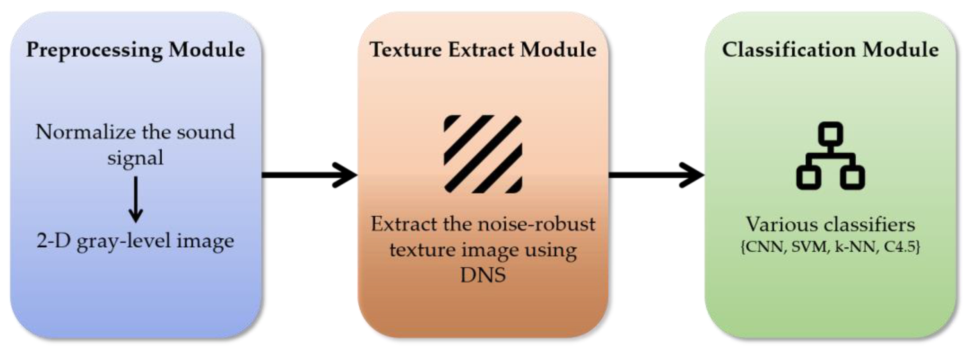
Figure 1. Overall system structure of the proposed method.
Symmetry 10 00402 g001
Figure 2. Conversion of two-dimensional gray-level image from a one-dimensional sound signal.
Symmetry 10 00402 g002
Figure 3. Process of extracting texture image using the dominant neighborhood structure (DNS) algorithm.
Symmetry 10 00402 g003
Figure 4. Convolutional neural network (CNN) structure for sound event classification.
Symmetry 10 00402 g004
Figure 5. Sound waveform acquired from railway-point machine: (a) normal event, (b) gravel event, (c) ice-covered event, and (d) unscrewed event. Horizontal axis shows the time axis. and vertical axis displays the sound signal in dB.
Symmetry 10 00402 g005aSymmetry 10 00402 g005b
Figure 6. Texture image of different types of events in railway-point machine: (a) normal event, (b) gravel event, (c) ice-covered event, and (d) unscrewed event.
Symmetry 10 00402 g006
Figure 7. The two-step process of transforming sound signals into a texture image. The first step is the process of converting a sound signal into a 2D gray-level image, and the second step is the process of creating a noise-robust texture image by applying DNS: (a) noise-free (normal event), (b) SNR 18, (c) SNR 0, (d) wind, and (e) rain.
Symmetry 10 00402 g007
Figure 8. Structural similarity (SSIM) comparison graph before and after applying DNS to railway-point-machine sound data under various noise conditions.
Symmetry 10 00402 g008
Figure 9. Sound waveforms acquired for the case of respiratory diseases: (a) normal (grunt) event, (b) postweaning multisystemic wasting syndrome (PMWS) event, (c) porcine reproductive and respiratory syndrome (PRRS) event, and (d) mycoplasma hyopneumoniae (MH) event. Horizontal axis shows the time axis and vertical axis shows the sound signal in dB.
Symmetry 10 00402 g009
Figure 10. Texture images of different types of events in the pigsty: (a) normal (grunt) event, (b) PMWS event, (c) PRRS event, and (d) MH event.
Symmetry 10 00402 g010
Figure 11. Texture image of a normal (grunt) sound event in a noisy environment: (a) SNR 18, (b) SNR 0, (c) strong footstep, and (d) door opening.
Symmetry 10 00402 g011
Figure 12. SSIM comparison graph before and after applying DNS to porcine sound data under various noise conditions.
Symmetry 10 00402 g012
Table 1. Basic statistics of environmental noise on railway-point-machine sound data.
Bird ChirpingHelicopterWindRain
SNR (dB)38.114614.531711.33208.4212
Mean Intensity–1.5 × 10−54.2 × 10−6–1.9 × 10⁻⁵–1.3 × 10⁻⁵
Max Intensity0.00970.24290.28490.2560
Min Intensity–0.0103–0.2724–0.2559–0.2863
Table 2. Classification results of the proposed method on railway-point-machine sound data under various noise conditions.
Noise ConditionsF1 Score
CNNSupport Vector Machine (SVM)k-Nearest Neighbors (k-NN)C4.5
SNR 180.99320.98610.90490.8781
SNR 150.99320.98660.89960.8666
SNR 120.99320.98680.89710.8578
SNR 90.99060.98510.89480.8481
SNR 60.99060.98530.88820.7993
SNR 30.98550.98320.88210.7882
SNR 00.97450.97320.88270.7438
Bird chirping0.99150.98510.89720.9617
Helicopter0.98980.98380.89620.8521
Wind0.98810.98160.88670.8226
Rain0.97790.97310.88220.7969
Average0.98800.98270.89200.8377
Standard deviation0.00630.00500.00790.0576
Table 3. Comparison of the F1 score of feature-extraction methods on railway-point-machine sound data.
Noise ConditionsF1 score
Proposed MethodModulation [16]Mel-Frequency Cepstral Coefficients (MFCC) [15]Modulation + MFCC [16]
SNR 180.99320.59020.59120.5953
SNR 150.99320.54620.54650.5469
SNR 120.99320.52060.52040.5272
SNR 90.99060.24150.31720.4366
SNR 60.99060.24150.24150.2415
SNR 30.98550.24150.24150.2415
SNR 00.97450.24150.24150.2415
Bird chirping0.99150.97340.99490.9898
Helicopter0.98980.97340.97270.9768
Wind0.98810.96240.96090.9715
Rain0.97790.32530.37760.2415
Average0.98800.53250.54600.5464
Standard deviation0.00630.30970.30290.3081
Table 4. Basic statistics of the environmental noise on porcine sound data.
Weak FootstepsRadio OperationStrong FootstepsDoor Opening
SNR (dB)9.11728.79717.46814.6820
Mean Intensity2.9 × 10−5–9.5 × 10⁻⁶–1.1 × 10⁻⁵–3.7 × 10⁻⁵
Max Intensity0.45940.36820.91980.8978
Min Intensity–0.5862–0.3615–0.9794–0.8593
Table 5. Classification of the proposed method on porcine sound data under various noise conditions.
Noise ConditionsF1 Score
CNNSVMk-NNC4.5
SNR 180.99390.99010.99190.9331
SNR 150.99390.98960.99190.9195
SNR 120.99390.98750.99190.8891
SNR 90.99250.98310.98970.8681
SNR 60.98970.95480.90150.7935
SNR 30.97090.89090.83750.7856
SNR 00.86430.88840.82710.7469
Weak footsteps0.98770.98290.98260.8834
Radio operation0.94100.97090.96540.8564
Strong footsteps0.97480.95540.94560.8471
Door opening0.91960.87240.88590.8381
Average0.96570.95150.93740.8510
Standard deviation0.04160.04530.06370.0573
Table 6. Comparison of the F1 score for feature extraction methods on porcine sound data.
Noise ConditionsF1 Score
Proposed MethodModulation [16]MFCC [9]Modulation + MFCC [16]
SNR 180.99390.86650.83650.8993
SNR 150.99390.86710.81610.8611
SNR 120.99390.83430.76530.8435
SNR 90.99250.81390.72770.8089
SNR 60.98970.79710.67520.7997
SNR 30.97090.73770.62790.7514
SNR 00.86430.71120.53540.7191
Weak footsteps0.98770.88330.79020.9232
Radio operation0.94100.80510.78810.8263
Strong footsteps0.97480.84950.76380.8949
Door opening0.91960.71670.69270.7258
Average0.96570.80750.72900.8230
Standard deviation0.04160.06150.08990.0700