A Note on Ordering Probability Distributions by Skewness

Abstract

This paper describes a complementary tool for fitting probabilistic distributions in data analysis. First, we examine the well known bivariate index of skewness and the aggregate skewness function, and then introduce orderings of the skewness of probability distributions. Using an example, we highlight the advantages of this approach and then present results for these orderings in common uniparametric families of continuous distributions, showing that the orderings are well suited to the intuitive conception of skewness and, moreover, that the skewness can be controlled via the parameter values.

1. Introduction

Detailed knowledge of the characteristics of probability models is desirable (if not essential) if data are to be modeled properly. In studying these properties, many authors have considered orderings within probability distribution families, according to diverse measuring criteria. The usual approach taken by researchers in this field is to evaluate or measure one or more theoretical characteristics of a given distribution and to study the effect produced by the value of its parameters on this measurement. In actuarial science, stochastic orders are widely used in order to make risk comparisons [1].

Some parametric distributions can be ordered according to the evaluation made of a given property, merely by comparing some of its parameters. Although most related orders are actually preorders, each one presents interesting applications. Many studies have been conducted in this area, and the following are particularly significant: Lehmann (1955) [2], which is of seminal importance; Arnold (1987) [3], who compared random variables according to stochastic ordering in a particular Lorenz order; Shaked and Shanthikumar (2006) [1], on stochastic orders; Nanda and Shaked (2001) [4], on reversed hazard rate orders; Ramos-Romero and Sordo-Díaz (2001) [5], on the likelihood ratio order; and Gupta and Aziz (2010) [6], on convex orders.

In this paper, we study the relationship between the skewness of some parametric distributions and the value of one of their parameters. The first question to be addressed is that of measuring the skewness. In this respect, Oja (1981) [7] introduced a set of axioms to be verified by any measurement of skewness considered. These axioms were established for indexes of skewness with one main constraint: that the skewness of a distribution should be evaluated by a single real number. This point is discussed below.

Many authors have proposed and obtained different descriptive elements to measure skewness (see, for instance, [8,9,10,11,12,13]). Ref [10] suggested a measurement of skewness corresponding to the (unique) mode, M, given by the following index:

$${\gamma }_M\left(F\right)=1-2F\left(M\right).$$

(1)

Ref [10] applied this index to ordering the gamma, log-logistic, lognormal and Weibull families of distributions by their skewness, taking into account the feasible values of their respective parameters. Index (1), which is proven to satisfy those axioms derived from Oja (1981) [7], is also recommended in [14] as a (very) good index of skewness. However, notice that (1) only compares the probability weight on the left side of a central point (the mode) with the value $1/2$, but it does not account for how the weights are distributed to each side of the centre.

García et al. (2015) [15] introduced some further elements to be incorporated into the list of skewness measurements of a probability distribution. According to these authors, given a unimodal probability distribution $F\left(x\right)$, its skewness is considered to be a local function of a given distance, z, from the mode, M. For such a distance, and given the interval $\left[M-z,M+z\right]$, the aggregate skewness function, ${\nu }_F\left(z\right)$, compares the probability weight of F at either side of the interval:

$${\nu }_F\left(z\right)=\mathrm{Pr}\left(X>M+z\right)-\mathrm{Pr}\left(X<M-z\right),$$

(2)

where $z\ge 0$. Thus, the (maximum) right skewness of the distribution F and its (minimum) left skewness are respectively given by

$$S^{+}\left(F\right)=\underset{z\ge 0}{max}{\nu }_F\left(z\right),S^{-}\left(F\right)=\underset{z\ge 0}{min}{\nu }_F\left(z\right).$$

(3)

The distances, $z_p$ and $z_n$, where these extreme values are achieved, are termed the critical distances to the mode. As the skewness function is bounded inside the interval $\left[-1,1\right]$ and ${\nu }_F\left(\infty \right)=0$, the bivariate index ${\displaystyle \left(S^{-}\left(F\right),S^{+}\left(F\right)\right)}$ belongs to $\left[-1,0\right]\times \left[0,1\right]$. A given distribution function F such that ${\nu }_F\left(z\right)\ge 0$ for all $z\ge 0$ is said to be only skewed to the right; and if ${\nu }_F\left(z\right)\le 0$ for all $z\ge 0$, it is said to be only skewed to the left.

The relationship $F{<}_{c}G$ (F $c-$precedes G) means that $G^{-1}\left[F\left(x\right)\right]$ is a convex function. For a continuous distribution F, the bivariate measurement of skewness ${\displaystyle \left(S^{-}\left(F\right),S^{+}\left(F\right)\right)}$ verifies the following properties, where $aF+b$ and $-F$ mean the distributions of the corresponding transformation of a random variable that is $F-$distributed:

• ${\displaystyle \left(S^{-}\left(F\right),S^{+}\left(F\right)\right)=\mathbf{0},}$ for any symmetric distribution F.
• ${\displaystyle \left(S^{-}\left(aF+b\right),S^{+}\left(aF+b\right)\right)=\left(S^{-}\left(F\right),S^{+}\left(F\right)\right)}$, for all $a>0$, $-\infty <b<\infty$.
• ${\displaystyle \left(S^{-}\left(-F\right),S^{+}\left(-F\right)\right)=\left(-S^{+}\left(F\right),-S^{-}\left(-F\right)\right)}$.
• If $F{<}_{c}G$, then ${\displaystyle \left(S^{-}\left(F\right),S^{+}\left(F\right)\right)\le \left(S^{-}\left(G\right),S^{+}\left(G\right)\right),}$ understood as vector dominance.

These properties can be considered as a vectorial interpretation of the axioms given by Oja (1981) [7].

As it is easily proven that ${\nu }_F\left(0\right)={\gamma }_M\left(F\right)$, we can establish that (2) and (3) give considerably clearer and more complete information than (1) about the skewness of any distribution function.

Most families of continuous distributions are only skewed to the right (or only to the left), while doubles-sign skewness is abundant within the discrete families, as shown in [15]. Nevertheless, the joint use of the function (2) and the bivariate index (3) makes it possible to improve the ordering of the skewness-based distribution discussed in [10], as can be seen in the following example.

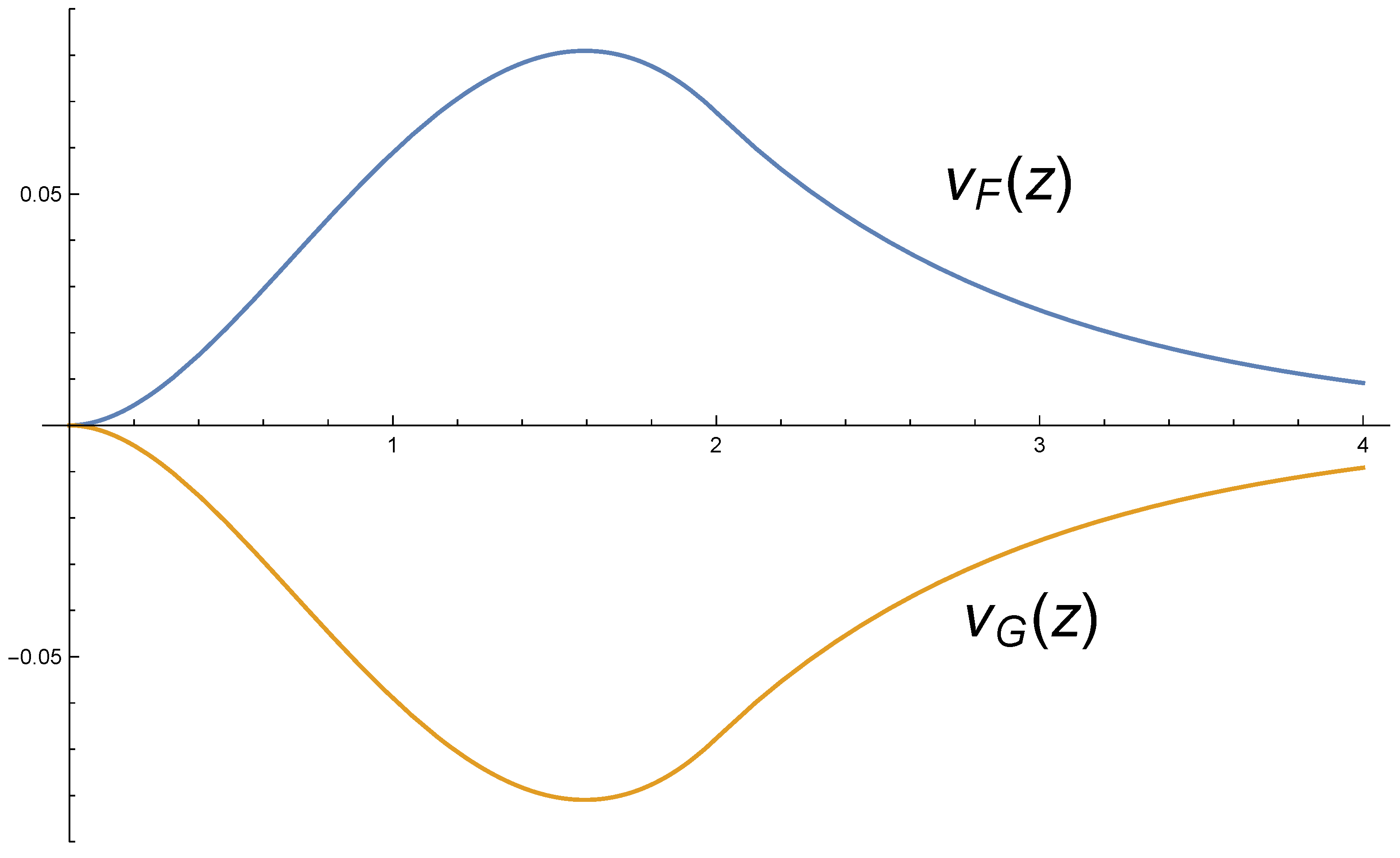
Example 1.

Assume the following random variable $X\in [-2,\infty )$ with PDF given by:

$${\displaystyle f\left(x\right)=\left\{\begin{array}{cc}{\displaystyle \frac{1}{4}}x+{\displaystyle \frac{1}{2}},& -2\le x<0;\\ {\displaystyle \frac{1}{2}}\exp \left(-x\right),& x\ge 0.\end{array}\right.}$$

Assume also the PDF, $g\left(y\right)$ of $Y=-X$. Then, ${\displaystyle {\gamma }_M\left(F\right)=0={\gamma }_M\left(G\right).}$ That is, according to coefficient ${\gamma }_M\left(·\right)$, both distributions have the same null skewness, although they do not even have a symmetric support set.

However, using expression (2), we find that

$${\displaystyle {\nu }_F\left(z\right)=\left\{\begin{array}{cc}{\displaystyle \frac{1}{2}}\exp \left(-z\right)-{\displaystyle \frac{1}{8}}{\left(z-2\right)}^2,& 0\le z<2;\\ {\displaystyle \frac{1}{2}}\exp \left(-z\right),& z\ge 2,\end{array}\right.}$$

and ${\nu }_G\left(z\right)=-{\nu }_F\left(z\right),$ for all $z\ge 0$. These functions are plotted in Figure 1, where it can be seen that ${\nu }_F\left(z\right)\ge {\nu }_G\left(z\right)$ for all $z\ge 0$, $S^{+}\left(F\right)=-S^{-}\left(G\right)\ne 0$ and $S^{-}\left(F\right)=0=S^{+}\left(G\right)$. Clearly, the information about skewness obtained from the aggregate skewness function $\nu \left(z\right)$ and the indices $S^{+}\left(·\right)$ and $S^{-}\left(·\right)$ is considerably more comprehensive than that obtained from ${\gamma }_M\left(·\right)$.

Outline

In applied statistical analysis, it is useful to have a large catalogue of plausible distributions with which to fit the data. According to García et al. (2015) [15], common measures of skewness can be complemented with a bivariate index of positive–negative skewness, and the authors show that the mode is the relevant central value to study both right and left skewness. In this paper, we extend the tool-box approach to fit data from probability distributions, introducing two orderings that are deduced from the skewness measures given in [15]. The first of those orderings is based on the positive part of the bivariate index of skewness, which in many instances coincides with the well known ${\gamma }_M\left(F\right)$. Nevertheless, the differences can be highly significant, as in the previous example. The second, more noteworthy, order is based on the skewness function ${\nu }_F\left(z\right)$ and meets the first of the conditions, but not the reciprocal.

There are two reasons for ordering a family of distributions according to a given measurement of skewness. Firstly, as a property of the distribution, this ordering allows us to control its skewness by the appropriate selection of the parameter. When this is done (and the parameter is readily determined), the theoretical results have immediate applications in the data-fitting process. Secondly, when a given family of distributions is conceived as being more or less skewed according to the value of a parameter, and a measurement of skewness ratifies the ordering, it may be concluded that the functioning of this measurement provides a reasonably good fit with an intuitive conception of skewness.

The rest of this paper is organized as follows. In Section 2, we study the aggregate skewness function and the resultant skewness-based ordering of the gamma, log-logistic, lognormal, Weibull and asymmetric Laplace families of continuous probability distributions. In Section 3, we study the ordering of two of the most well-known distributions commonly used in PERT methods: the beta and the asymmetric triangular distributions. Finally, conclusions are presented in Section 4.

2. Families of Uniparametric Distributions Ordered by Skewness

Let F and G be unimodal distribution functions, with no centre or scale parameters, and modes $M_F$ and $M_G,$ respectively. We compare their respective skewness by two different criteria.

Definition 1.

If

$${\nu }_F\left(z\right)-{\nu }_G\left(z\right)\ge 0,\forall z\ge 0,$$

(4)

then we say that F has equal or more aggregate skewness to the right at any point than $G.$ We denote this by $F{\ge }_{\nu }G$.

Definition 2.

If $F$ and G are both skewed only to the right, we say that F has equal or more maximum aggregate skewness to the right than G when

$$S^{+}\left(F\right)-S^{+}\left(G\right)\ge 0,$$

(5)

and we denote this by $F{\ge }_{+}G$.

With these definitions, it immediately follows that:

Proposition 1.

If $F{\ge }_{\nu }G,$ then $F{\ge }_{+}G.$

The reverse implication is not true in general.

Proof. 

The proof follows immediately from the definitions given in (4) and (5). ☐

In the next section, we consider some well known uniparametric families of continuous distributions, with no centre or scale parameters but depending on a skewness parameter, and examine whether they are ordered by aggregate skewness, or by maximum aggregate skewness. The gamma family is a very broad one, which includes many other well known distributions as particular cases. A study of the log-logistic, lognormal, Weibull and asymmetric Laplace families, one by one and in turn, when not included inside the previous one, will produce widely varying results.

2.1. Uniparametric Gamma Distributions

Let X be a uniparametric gamma distributed random variable, $G\left(\alpha \right)$. That is, its CDF $G\left(x;\alpha \right)$ is given by

$$G\left(x;\alpha \right)=\frac{1}{\mathrm{\Gamma }\left(1+\alpha \right)}{\int }_0^x{t}^{\alpha }{e}^{-t}dt,$$

(6)

for $x>0$, where $-1<\alpha <\infty$, and the mode is given by $M=max\left\{\alpha ,0\right\}$. Then, for $-1<\alpha \le 0$, the density function decreases on x along the positive real line and we obtain that

$${\nu }_G\left(z;\alpha \right)=1-G\left(z;\alpha \right)=\frac{1}{\mathrm{\Gamma }\left(1+\alpha \right)}{\int }_z^{\infty }{t}^{\alpha }{e}^{-t}dt.$$

In these cases, ${\nu }_G\left(z;\alpha \right)$ is a decreasing function on z, and $S^{+}\left(G\left({\alpha }_1\right)\right)={\nu }_G\left(0;{\alpha }_1\right)=1.$

Proposition 2.

Let $G\left({\alpha }_1\right)$ and $G\left({\alpha }_2\right)$ be gamma distributions with CDF as in (6). Then:

1. 

If $-1<{\alpha }_1<{\alpha }_2<0$, then $G\left({\alpha }_2\right){\ge }_{\nu }G\left({\alpha }_1\right).$

2. 

If $0<{\alpha }_1<{\alpha }_2$, then $G\left({\alpha }_1\right){\ge }_{+}G\left({\alpha }_2\right).$

Proof. 

Part 1. We can write

$${\nu }_G\left(z;{\alpha }_1\right)-{\nu }_G\left(z;{\alpha }_2\right)=G\left(z;{\alpha }_2\right)-G\left(z;{\alpha }_1\right).$$

By denoting ${\alpha }_2={\alpha }_1+\epsilon$, $\epsilon >0$, and then considering ${\displaystyle u\left(z\right)=\frac{d}{dz}\left[{\nu }_G\left(z;{\alpha }_1\right)-{\nu }_G\left(z;{\alpha }_2\right)\right],}$ we obtain

$$u\left(z\right)=\frac{z^{{\alpha }_2}{e}^{-z}}{\mathrm{\Gamma }\left(1+{\alpha }_2\right)}-\frac{z^{{\alpha }_1}{e}^{-z}}{\mathrm{\Gamma }\left(1+{\alpha }_1\right)}=z^{{\alpha }_1}{e}^{-z}\left[\frac{z^{\epsilon }\mathrm{\Gamma }\left(1+{\alpha }_1\right)-\mathrm{\Gamma }\left(1+{\alpha }_2\right)}{\mathrm{\Gamma }\left(1+{\alpha }_2\right)\mathrm{\Gamma }\left(1+{\alpha }_1\right)}\right].$$

Therefore, $u\left(z\right)=0$ when

$$z=z_0={\left[\frac{\mathrm{\Gamma }\left(1+{\alpha }_2\right)}{\mathrm{\Gamma }\left(1+{\alpha }_1\right)}\right]}^{1/\epsilon },$$

$u\left(z\right)$ is negative for $0<z<z_0$, and positive for $z>z_0$. Also, ${\nu }_G\left(0^{+};{\alpha }_1\right)-{\nu }_G\left(0^{+};{\alpha }_2\right)=0$, ${\nu }_G\left(\infty ;{\alpha }_1\right)-{\nu }_G\left(\infty ;{\alpha }_2\right)=0$. Then,

$$\begin{array}{ccc}\hfill {\nu }_G\left(z_0;{\alpha }_1\right)-{\nu }_G\left(z_0;{\alpha }_2\right)& =& \frac{1}{\mathrm{\Gamma }\left(1+{\alpha }_1\right)\mathrm{\Gamma }\left(1+{\alpha }_2\right)}{\int }_0^{x_0}{t}^{{\alpha }_1}{e}^{-t}\left[\mathrm{\Gamma }\left(1+{\alpha }_1\right)t^{\epsilon }-\mathrm{\Gamma }\left(1+{\alpha }_2\right)\right]dt,\hfill \end{array}$$

is the integral of a negative function, so it is negative, and the proof is complete.

Part 2. For $0<\alpha <\infty$, we have that

$${\displaystyle {\nu }_G\left(z;\alpha \right)=\left\{\begin{array}{cc}\frac{1}{\mathrm{\Gamma }\left(1+\alpha \right)}\left({\int }_{z+\alpha }^{\infty }{t}^{\alpha }{e}^{-t}dt-{\int }_0^{\alpha -z}{t}^{\alpha }{e}^{-t}dt\right),& 0\le z<\alpha ,\\ \frac{1}{\mathrm{\Gamma }\left(1+\alpha \right)}{\int }_{z+\alpha }^{\infty }{t}^{\alpha }{e}^{-t}dt,& z\ge \alpha .\end{array}\right.}$$

and,

$$\frac{d{\nu }_G}{dz}=\left\{\begin{array}{cc}\frac{1}{\mathrm{\Gamma }\left(1+\alpha \right)}\left[{\left(\alpha -z\right)}^{\alpha }{e}^{-\left(\alpha -z\right)}-{\left(\alpha +z\right)}^{\alpha }{e}^{-\left(\alpha +z\right)}\right],& 0\le z<\alpha ,\\ \frac{-1}{\mathrm{\Gamma }\left(1+\alpha \right)}{z}^{\alpha }{e}^{-z},& z\ge \alpha .\end{array}\right.$$

Then, clearly we have that $d{\nu }_G/dz<0$ for all $z\ge \alpha$. For $0\le z<\alpha$, if we denote

$$w\left(z\right)={\left(\alpha -z\right)}^{\alpha }{e}^z-{\left(\alpha +z\right)}^{\alpha }{e}^{-x},$$

then the sign of $d{\nu }_G/dz$ is the sign of $w\left(x\right)$. As $w\left(0\right)=0$, $w\left(\alpha \right)=-{\left(2\alpha \right)}^{\alpha }{e}^{-\alpha }<0$, and

$$\frac{dw}{dz}=z{\left(z+\alpha \right)}^{\alpha -1}{e}^{-z}-z{\left(\alpha -z\right)}^{\alpha -1}{e}^z\le 0,$$

we conclude that ${\nu }_G$ is a decreasing function on $z\ge 0$ and $S^{+}\left(G\left(\alpha \right)\right)={\nu }_G\left(0;\alpha \right).$

$$S^{+}\left(G\left(\alpha \right)\right)=\frac{\mathrm{\Gamma }\left(1+\alpha ,\alpha \right)}{\mathrm{\Gamma }\left(1+\alpha \right)},$$

where $\mathrm{\Gamma }\left(1+\alpha ,\alpha \right)$ is the incomplete Gamma function, and then $S^{+}\left(G\left(\alpha \right)\right)$ is a decreasing function on $\alpha$, when $\alpha \to \infty$. Nevertheless, a simple plotting of the functionals ${\nu }_G\left(z;{\alpha }_i\right)$ for any $0<{\alpha }_1<{\alpha }_2$ shows that both functionals cross each other and that they are not ordered by ”${\ge }_{\nu }$”. Thus, the proof is completed. ☐

2.2. Log–Logistic Distributions

The CDF of a uniparametric log–logistic distributed random variable X is given by

$$F_{LL}\left(x;\theta \right)={\left(1+x^{-\theta }\right)}^{-1},$$

(7)

for $x>0$, with $\theta >0$. The mode of these distributions depends on $\theta$. If $0<\theta \le 1$, then $M=0$, and

$${\nu }_{LL}\left(z;\theta \right)=\frac{1}{1+z^{\theta }},$$

and $S^{+}\left(F_{LL}\left(\theta \right)\right)=1$. The functionals ${\nu }_{LL}\left(z;\theta \right)$ for different values of $\theta$ inside the rank cross each other at $z=1$, and these distributions are ordered neither by skewness function nor by skewness indexes. Nevertheless, for $\theta >1$, the mode is

$$0<M={\left(\frac{\theta -1}{\theta +1}\right)}^{1/\theta }<1.$$

(8)

Notice that M is an increasing function of $\theta$ when $\theta >1,$ because

$$\frac{dM}{d\theta }=M·\left[\frac{2}{\left({\theta }^2-1\right)\theta }-\frac{1}{{\theta }^2}\ln \frac{\theta -1}{\theta +1}\right]>0.$$

(9)

When $\theta >1$, it is also known from Arnold and Groeneveld (1995) that

$${\nu }_{LL}\left(0;\theta \right)=\frac{1}{\theta }.$$

As ${\nu }_L\left(z;\theta \right)$ is a decreasing function, it is then stated that $1<{\theta }_1<{\theta }_2$ implies ${\displaystyle F_{LL}\left({\theta }_1\right){\ge }_{+}{F}_{LL}\left({\theta }_2\right)}$. Furthermore, the skewness functions are ordered, as we prove below.

Proposition 3.

Let be ${\displaystyle F_{LL}\left({\theta }_1\right)}$ and ${\displaystyle F_{LL}\left({\theta }_2\right)}$ log-logistic distributions with CDF as in (7), where $1<{\theta }_1<{\theta }_2$. Then,

$$F_{LL}\left({\theta }_1\right){\ge }_{\nu }{F}_{LL}\left({\theta }_2\right).$$

(10)

Proof. 

Let $\theta >1$. Then,

$${\nu }_{LL}\left(z;\theta \right)=\left\{\begin{array}{cc}{\displaystyle \frac{1-{\left(M^2-z^2\right)}^{\theta }}{1+{\left(M+z\right)}^{\theta }+{\left(M-z\right)}^{\theta }+{\left(M^2-z^2\right)}^{\theta }}},& 0\le z\le M,\\ {\displaystyle \frac{1}{1+{\left(M+z\right)}^{\theta }}},& z>M,\end{array}\right.$$

If we consider $1<{\theta }_1<{\theta }_2$, such that the respective modes verify $0<M_1<M_2<1$, we can then denote

$$a={\left(M_1-z\right)}^{{\theta }_1}<b={\left(M_1+z\right)}^{{\theta }_1},$$

$$c={\left(M_2-z\right)}^{{\theta }_2}<d={\left(M_2+z\right)}^{{\theta }_2}.$$

and consider the function h given by

$${\displaystyle h\left(\theta \right)={\left(M\pm z\right)}^{\theta },0\le z\le M,}$$

with M as in (8). Then,

$$\begin{array}{ccc}\hfill \frac{dh}{d\theta }& =& \frac{{\left(M\pm z\right)}^{\theta -1}}{\theta {\left(\theta +1\right)}^2}\left(\frac{2\theta }{M^{\theta -1}}+\theta {\left(1+\theta \right)}^2\left(M\pm z\right)\ln \left(M\pm z\right)+{\left(1+\theta \right)}^{2}M\ln \frac{\theta +1}{\theta -1}\right),\hfill \end{array}$$

For $z<M,$ this implies that $a<c$, $b<d$. With this notation, we can write ${\nu }_{LL}\left(z;{\theta }_1\right)-{\nu }_{LL}\left(z;{\theta }_2\right)$ as follows.

Firstly, for $0\le z\le M_1$,

$$\begin{array}{ccc}\hfill {\nu }_{LL}\left(z;{\theta }_1\right)-{\nu }_{LL}\left(z;{\theta }_2\right)& =& \frac{1-ab}{\left(1+a\right)\left(1+b\right)}-\frac{1-cd}{\left(1+c\right)\left(1+d\right)}\hfill \\ & =& \frac{\left(c-a\right)+\left(d-b\right)+ac\left(d-b\right)+bd\left(c-a\right)+2\left(cd-ab\right)}{\left(a+1\right)\left(b+1\right)\left(c+1\right)\left(d+1\right)}>0.\hfill \end{array}$$

Secondly, for $M_1<z\le M_2$, we only need to compare $d-b$, because

$$\begin{array}{ccc}\hfill {\nu }_{LL}\left(z;{\theta }_1\right)-{\nu }_{LL}\left(z;{\theta }_2\right)& =& \frac{1}{1+b}-\frac{1-cd}{\left(1+c\right)\left(1+d\right)}\hfill \\ & =& \frac{c+\left(d-b\right)+2cd+bcd}{\left(1+b\right)\left(1+c\right)\left(1+d\right)}>0.\hfill \end{array}$$

Finally, when $z>M_2$,

$${\nu }_{LL}\left(z;{\theta }_1\right)-{\nu }_{LL}\left(z;{\theta }_2\right)=\frac{1}{1+b}-\frac{1}{1+d}=\frac{d-b}{\left(1+b\right)\left(1+d\right)}>0.$$

Hence, the proof is completed. ☐

2.3. Lognormal Variance Distributions

$$LN\left(x;\sigma \right)=\mathrm{\Phi }\left(\frac{\ln x}{\sigma }\right),$$

(11)

for $x,\sigma >0$, where $\mathrm{\Phi }\left(·\right)$ is the standard normal distribution function. The mode is given by $M_{\sigma }=\exp \left(-{\sigma }^2\right)$ and

$${\nu }_{LN}\left(z;\sigma \right)=1-\mathrm{\Phi }\left(\frac{\ln \left[z+\exp \left(-{\sigma }^2\right)\right]}{\sigma }\right)-\mathrm{\Phi }\left(\frac{\ln \left[\exp \left(-{\sigma }^2\right)-z\right]}{\sigma }\right).$$

Proposition 4.

Let $LN\left({\sigma }_1\right)$ and $LN\left({\sigma }_2\right)$ be lognormal distributions with CDF as in (11), where $0<{\sigma }_1<{\sigma }_2$. Then,

$$LN\left({\sigma }_2\right){\ge }_{\nu }LN\left({\sigma }_1\right).$$

Proof. 

For $0<{\sigma }_1<{\sigma }_2,$ the corresponding modes are $M_1>M_2$, and

$$\mathrm{\Phi }\left(\frac{\ln \left(z+M_1\right)}{{\sigma }_1}\right)>\mathrm{\Phi }\left(\frac{\ln \left(z+M_2\right)}{{\sigma }_2}\right),$$

$$\mathrm{\Phi }\left(\frac{\ln \left(-z+M_1\right)}{{\sigma }_1}\right)>\mathrm{\Phi }\left(\frac{\ln \left(-z+M_2\right)}{{\sigma }_2}\right),$$

because $\mathrm{\Phi }$ is a strictly increasing function. Thus, we obtain that ${\nu }_{LN}\left(z;{\sigma }_1\right)>{\nu }_{LN}\left(z;{\sigma }_2\right)$ for all $z>0$ and the proof is completed. ☐

2.4. Uniparametric Weibull Distributions

Consider the uniparametric Weibull distributions family given by the CDF

$$W\left(x;c\right)=1-\exp \left(-x^c\right),x>0,c>0.$$

(12)

The mode is known to be at 0, for $c\le 1$ (as a limit, when $c<1$) and at

$$0<M_c={\left(\frac{c-1}{c}\right)}^{1/c}<1,$$

for $c>1$. The expression for ${\nu }_W$ is given by

$${\nu }_W\left(z;c\right)=\left\{\begin{array}{cc}\exp \left[-{\left(M_c+z\right)}^c\right]+\exp \left[-{\left(M_c-z\right)}^c\right]-1,& 0<z<M_c\\ \exp \left[-{\left(M_c+z\right)}^c\right],& z\ge M_c\end{array}\right.$$

On the one hand, when $c<1$, note that ${\nu }_{W\left(c\right)}\left(1\right)=e^{-1}$, so all these functions intersect at this point. Graphically, it can be seen that there is no ordering by “${\ge }_{\nu }$”, and also that $S^{+}\left(W\left(c\right)\right)=1$, when $c<1$. On the other hand, for $1\le c_1<c_2$, the following result is obtained.

Proposition 5.

Let $W\left(c_1\right)$ and $W\left(c_2\right)$ be Weibull distributions with $1\le c_1<c_2$ and CDF as in (12). Then,

$$W\left(c_1\right){\ge }_{\nu }W\left(c_2\right).$$

Proof. 

For $1\le c_1<c_2$, the corresponding modes are $M_1<M_2$. Then, for $0<z<M_1,$

$${\displaystyle {\nu }_W\left(z;c_1\right)-{\nu }_W\left(z;c_2\right)=\left\{\exp \left[-{\left(M_1+z\right)}^{c_1}\right]-\exp \left[-{\left(M_2+z\right)}^{c_2}\right]\right\}}$$

$$+\left\{\exp \left[-{\left(M_1-z\right)}^{c_1}\right]-\exp \left[-{\left(M_2-z\right)}^{c_2}\right]\right\}>0,$$

because each part of the expression inside brackets $\left\{·\right\}$ is positive. If we take $M_1\le z<M_2$, then

$${\nu }_W\left(z;c_1\right)-{\nu }_W\left(z;c_2\right)=\left\{\exp \left[-{\left(M_1+z\right)}^{c_1}\right]-\exp \left[-{\left(M_2+z\right)}^{c_2}\right]\right\}$$

$$+\left\{1-\exp \left[-{\left(M_2-z\right)}^{c_2}\right]\right\}>0,$$

for a similar reason. Finally, if we take $z>M_2$, then

$${\nu }_W\left(z;c_1\right)-{\nu }_W\left(z;c_2\right)=\exp \left[-{\left(M_1+z\right)}^{c_1}\right]-\exp \left[-{\left(M_2+z\right)}^{c_2}\right]>0,$$

and the proof is completed. ☐

2.5. Asymmetric Laplace Distributions

The asymmetric Laplace distribution has been introduced in the literature by different ways ([16,17]). In this paper we will use Kozubowski and Podgórski (2002) [18] (later refined in [19]) to refer it. This distribution is obtained by using the scheme introduced by Fernández and Steel (1998) [20] to produce skewness on a symmetric distribution. In this way, the pdf of a skewed or asymmetric Laplace distribution can be written in the form

$$f\left(x;\mu ,\sigma ,\kappa \right)=\left\{\begin{array}{cc}\frac{\sqrt{2}}{\sigma }\frac{\kappa }{1+{\kappa }^2}\exp \left[-\frac{\sqrt{2}}{\kappa \sigma }\left(\mu -x\right)\right],& x<\mu ,\\ \frac{\sqrt{2}}{\sigma }\frac{\kappa }{1+{\kappa }^2}\exp \left[-\frac{\kappa \sqrt{2}}{\sigma }\left(x-\mu \right)\right],& x\ge \mu ,\end{array}\right.$$

where $\sigma ,\kappa >0$, and $-\infty <\mu <\infty$. Then, we assign values $\left(0,1\right)$ to the centre and scale parameters ($\mu$ and $\sigma$, respectively) in order to study the aggregate skewness function, and the extreme right and left skewness indices then depend only on the skewness parameter $\kappa >0$. Thus, it is easily proven that:

• The aggregate skewness function of an $AL\left(\kappa \right)$ distribution can be written as

  $${\nu }_{AL}\left(z;\kappa \right)=\frac{1}{1+{\kappa }^2}\left[\exp \left(-\sqrt{2}\kappa z\right)-{\kappa }^2\exp \left(-\frac{\sqrt{2}}{\kappa }z\right)\right].$$
• ${\nu }_{AL}\left(z;\kappa \right)$ is an increasing negative function of z when $\kappa >1$, and it is a decreasing positive function of z when $0<\kappa <1$. ${\nu }_{AL,1}\left(z;1\right)=0$, for all $z\ge 0$. That is, any $AL$ distribution is skewed only to the right or to the left, depending on $\kappa$. In any case, the function verifies ${lim}_{z\to \infty }{\nu }_{AL}\left(z;\kappa \right)=0$ but, when $\kappa \ne 1$, the function never reaches that limit value. To prove these results, it is sufficient to note that

  $$\frac{d{\nu }_{AL}\left(z;\kappa \right)}{dz}=\frac{\sqrt{2}\kappa }{{\kappa }^2+1}\left[\exp \left(-\frac{\sqrt{2}}{\kappa }z\right)-\exp \left(-\sqrt{2}\kappa z\right)\right].$$
• At $z=0$, the skewness function takes the following value:

  $${\nu }_{AL}\left(0;\kappa \right)=\frac{1-{\kappa }^2}{1+{\kappa }^2}.$$

  Then, ${\nu }_{AL}\left(0;\kappa \right)$ is the value for $S^{+}\left(F_{AL}\left(\kappa \right)\right)$ or $S^{-}\left(F_{AL}\left(\kappa \right)\right)$, depending on its sign.
• ${\nu }_{AL}\left(z;\kappa \right)$ is a strictly decreasing function on $\kappa$. This is easily shown by means of

  $$\frac{d{\nu }_{AL}\left(z;\kappa \right)}{d\kappa }=-\frac{\sqrt{2}z{\kappa }^2+2\kappa +\sqrt{2}z}{{\left({\kappa }^2+1\right)}^2}\left[\exp \left(-\sqrt{2}\frac{z}{\kappa }\right)+\exp \left(-\sqrt{2}\kappa z\right)\right]<0,$$

  for all $z>0$, and all $\kappa >0$.

As a conclusion, we can enunciate the following Proposition, whose proof is straightforward and hence omitted.

Proposition 6.

Assume $0<{\kappa }_1<{\kappa }_2<\infty$, and let $F_{AL}\left({\kappa }_1\right)$ and $F_{AL}\left({\kappa }_2\right)$ be the respective asymmetric Laplace distributions. Then:

1. 

$F_{AL}\left({\kappa }_1\right){\ge }_{\nu }{F}_{AL}\left({\kappa }_2\right).$

2. 

If $0<{\kappa }_1<1$, then $F_{AL}\left({\kappa }_1\right)$ is skewed only to the right.

3. 

If ${\kappa }_1>1$, then $F_{AL}\left({\kappa }_1\right)$ is skewed only to the left.

3. The Beta and the AST Distributions

The methods for Project Management and Review Technique (PERT) are well known and widely applied when the needed activities for a given project must be ordered according to precedence in time. Some of these methods require modelling the time length of each activity as a random variable, following an expert’s opinion. The beta and the asymmetric triangular distributions are commonly used by engineers to describe these time lengths. In any case, the indications of the experts can be related to a maximum and a minimum values and a mode, often completed with further considerations about the shape and skewness of the PDF of the time random variable. Then, a deep study of the skewness of both families of probability distributions would be welcome to improve the model fit.

On the one hand, the asymmetric standard triangular distribution (ASTD) , free of center and scale parameters, depends on only one parameter $0\le \theta \le 1$, and has the pdf:

$$f\left(x|\theta \right)=\left\{\begin{array}{cc}2x{\theta }^{-1},& 0\le x\le \theta ,\\ 2\left(1-x\right){\left(1-\theta \right)}^{-1},& \theta \le x\le 1,\\ 0,& \mathrm{elsewhere}.\end{array}\right.$$

There is a large body of literature that shows the use of the ASTD in PERT methods (see [21] and [19] and cites therein). Note that cases $\theta =0,1$ are members of the beta family of distributions.

For $0<\theta <1$, the $ASTD\left(\theta \right)$ CDF can be written as follows:

$$F\left(x|\theta \right)=\left\{\begin{array}{cc}{x}^2{\theta }^{-1},& 0\le x\le \theta ,\\ \left(2x-x^2-\theta \right){\left(1-\theta \right)}^{-1},& \theta \le x\le 1.\end{array}\right.$$

As the mode is found to be at $x=\theta$, its skewness function is found to be

$${\nu }_{ASTD}\left(z;\theta \right)=\left(1-2\theta \right)-\frac{\left(1-2\theta \right)}{\theta \left(1-\theta \right)}{z}^2,$$

for $0\le z\le min\left\{\theta ,1-\theta \right\}.$ In the case $\theta =0.5$, the skewness function is null. Then, for $0<\theta <0.5$ and $\theta <z\le 1-\theta$,

$${\nu }_{ASTD}\left(z;\theta \right)=\frac{{\left(z-1+\theta \right)}^2}{1-\theta }.$$

In the case $0.5<\theta <1$, for $1-\theta <z\le \theta$,

$${\nu }_{ASTD}\left(z;\theta \right)=-\frac{{\left(\theta -z\right)}^2}{\theta },$$

and it is easily found that

$${\nu }_{ASTD}\left(z;\theta \right)=-{\nu }_{ASTD}\left(z;1-\theta \right),$$

(13)

for $0\le z<\infty$.

Some algebra allows to prove that, being $0<{\theta }_1<{\theta }_2<1$,

• $ASTD\left({\theta }_1\right){\ge }_{\nu }ASTD\left({\theta }_2\right).$
• If $0<{\theta }_i<0.5$, then $S_{ASTD}^{+}\left({\theta }_i\right)={\nu }_{ASTD}\left(0;{\theta }_i\right)=1-2{\theta }_i$, and $S_{ASTD}^{-}\left({\theta }_i\right)=0$.
• If $0.5<{\theta }_i<1$, then $S_{ASTD}^{+}\left({\theta }_i\right)=0$ and $S_{ASTD}^{-}\left({\theta }_i\right)={\nu }_{ASTD}\left(0;{\theta }_i\right)=1-2{\theta }_i$.

Therefore, the skewness of the ASTD distributions is completely controlled by the parameter $\theta .$

On the other hand, the pdf of a beta distribution is given by

$$f_B\left(x;\alpha ,\beta \right)=\frac{x^{\alpha -1}{\left(1-x\right)}^{\beta -1}}{B\left(\alpha ,\beta \right)},0\le x\le 1,$$

where $\alpha ,\beta >0$, and $B\left(·,·\right)$ is the beta function. Given that its CDF $F\left(x;\alpha ,\beta \right)$ verifies that $F\left(x;\alpha ,\beta \right)=1-F\left(x;\beta ,\alpha \right)$ and the sign of its skewness depends only on the condition $\beta \ge \alpha$ or $\beta \le \alpha$, we can study only the case $\beta >\alpha$.

We are interested on the cases $\alpha ,\beta >1$, where there is an unique mode $M,$

$$M=\frac{\alpha -1}{\alpha +\beta -2}\doteq b\left(\alpha ,\beta \right).$$

Hence, we only consider cases where $1<\alpha <\beta$, where there exists a right skewness; the cases $1<\beta <\alpha$, with left skewness, can be immediately deducted by taking the parameters in reverse.

Notice that $\mathrm{Pr}\left(X>M+z\right)>0$ requires $0\le z\le b\left(\beta ,\alpha \right)$, and that $\mathrm{Pr}\left(X<M-z\right)>0$ requires $0\le z\le b\left(\alpha ,\beta \right)$. Then,

$${\nu }_B\left(z;\alpha ,\beta \right)=\left\{\begin{array}{cc}1-I_{M+z}\left(\alpha ,\beta \right)-I_{M-z}\left(\alpha ,\beta \right)>0,& 0\le z\le b\left(\alpha ,\beta \right)\\ 1-I_{M+z}\left(\alpha ,\beta \right)>0,& b\left(\alpha ,\beta \right)<z\le b\left(\beta ,\alpha \right)\\ 0,& z>b\left(\beta ,\alpha \right),\end{array}\right.$$

(14)

where,

$$I_z\left(\alpha ,\beta \right)={\int }_0^z\frac{t^{\alpha -1}{\left(1-t\right)}^{\beta -1}dt}{B\left(\alpha ,\beta \right)}$$

is the well known Beta Regularized function.

Firstly, observe that

$${\nu }_B\left(0;\alpha ,\beta \right)=1-\frac{2}{B\left(\alpha ,\beta \right)}{\int }_0^M{x}^{\alpha -1}{\left(1-x\right)}^{\beta -1}dx,$$

and

$$\frac{1}{B\left(\alpha ,\beta \right)}{\int }_0^M{x}^{\alpha -1}{\left(1-x\right)}^{\beta -1}dx<\frac{1}{B\left(\alpha ,\beta \right)}{\int }_0^m{x}^{\alpha -1}{\left(1-x\right)}^{\beta -1}dx\approx \frac{1}{2},$$

where

$$m=\frac{\alpha -\frac{1}{3}}{\alpha +\beta -\frac{2}{3}}$$

is the approximate median of the distribution.

Secondly, if $0\le z\le b\left(\alpha ,\beta \right)<b\left(\beta ,\alpha \right),$ then

$$B\left(\alpha ,\beta \right)·\frac{d{\nu }_B\left(z;\alpha ,\beta \right)}{dz}=-{\left[b\left(\alpha ,\beta \right)+z\right]}^{\alpha -1}{\left[b\left(\beta ,\alpha \right)-z\right]}^{\beta -1}-{\left[b\left(\alpha ,\beta \right)-z\right]}^{\alpha -1}{\left[b\left(\beta ,\alpha \right)+z\right]}^{\beta -1},$$

which is negative within the rank of z. For $b\left(\alpha ,\beta \right)<z\le b\left(\beta ,\alpha \right)$,

$$B\left(\alpha ,\beta \right)·\frac{d{\nu }_B\left(z;\alpha ,\beta \right)}{dz}=-{\left[b\left(\alpha ,\beta \right)+z\right]}^{\alpha -1}{\left[b\left(\beta ,\alpha \right)-z\right]}^{\beta -1}<0.$$

Hence, for $0\le z\le b\left(\beta ,\alpha \right)$, ${\nu }_B\left(z;\alpha ,\beta \right)$ is a strictly decreasing continuous function with ${\nu }_B\left(0;\alpha ,\beta \right)>0$ and ${\nu }_B\left(b\left(\beta ,\alpha \right);\alpha ,\beta \right)=0.$

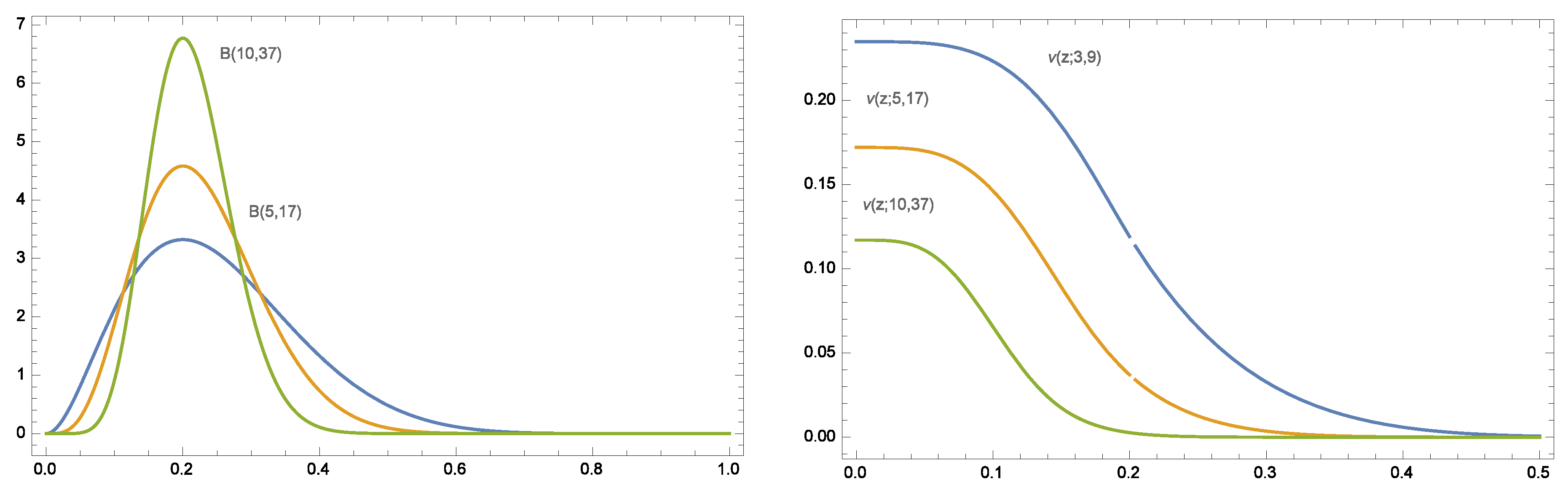
Now we focus on the family of Beta distributions with given mode, M. That is, we consider the subfamily of Beta distributions:

$$B\left(\alpha +1,1+\frac{1-M}{M}\alpha \right),$$

with $\alpha >0$. Then, with the aid of a proper software (we have used Wolfram Mathematica 10), one can obtain the derivative

$$\frac{\partial }{\partial \alpha }{\nu }_B\left(z;\alpha +1,1+\frac{1-M}{M}\alpha \right),$$

and maximize this function, in two cases:

First case, the constrains are $\alpha \ge 1,$$0<m<1/2,$$0\le z\le b\left(\alpha +1,1+\left(1-M\right)\alpha /M\right).$ The maximum value of the function is 0, and it is achieved when $M=0.5$, $\alpha \simeq 3.54147$, $z\simeq 0.309936$.

Second case, the constrain are $\alpha \ge 1,$$0<m<1/2,$$b\left(\alpha +1,1+\left(1-M\right)\alpha /M\right)<z\le b\left(1+\left(1-M\right)\alpha /M,\alpha +1\right).$ The maximum value of the function is $-5.07056\times {10}^{-6}$, and it is achieved when $M=0.123564$, $\alpha \simeq 1.62726$, $z\simeq 0.632457$.

With these results, we can conclude that ${\nu }_B\left(z;\alpha +1,1+\left(1-M\right)\alpha /M\right)$ decreases with the feasible values of $\alpha$. That way, the subsets of Beta distributions with fixed mode are ordered on skewness (see Figure 2). As the parameter values increase, these Beta distributions become less skewed.

4. Conclusions

In this paper two main objectives are achieved: on the one hand, the given examples show that the skewness function orders the mesh in good accordance with the intuitive conception of skewness. Moreover, these examples show that the skewness of a distribution obtained from certain parametric families can be controlled by reference to their parameters.

As we show, the function ${\nu }_F\left(z\right)$ facilitates the description of a random variable by means of a probability distribution, by making any skewness in the model easily observable and should be undertaken to examine the use of these properties in data fitting.

In practice, much can be learned from this model, but there remains the risk that it may be wrongly specified in real applications. Thus, in practice we must be willing to assume that the underlying distribution has a unique mode and belongs to a uniparametric family of distributions.

In many practical situations, the maximum skewness index coincides with the well known ${\gamma }_M\left(F\right)$, but this second index only takes into account the difference of probability weights at each side of the mode, while the first takes a value from the point where this difference is maximum. Moreover, the aggregate skewness function gives more accurate information about how the probability weight is distributed along both sides of the mode. Accordingly, the condition $F{\ge }_{\nu }G$ provides highly valuable information.