The Minimum Selection of Crowdsourcing Images under the Resource Budget

Abstract

Images crowdsourcing of mobile devices can be applied to many real-life application scenarios. However, this type of scenario application often faces issues such as the limitation of bandwidth, insufficient storage space, and the processing capability of CPU. These lead to only a few photos that can be crowdsourced. Therefore, it is a great challenge to use a limited number of resources to select photos and make it possible to cover the target area maximally. In this paper, the geographic and geometric information of the photo called data-unit is used to cover the target area as much as possible. Compared with traditional content-based image delivery methods, the network delay and computational costs can be greatly reduced. In the case of resource constraints, this paper uses the utility of photos to measure the coverage of the target area, and improves a photo utility calculation method based on data-unit. In the meantime, this paper proposes the minimum selection problem of images under the coverage requirements, and designs a selection algorithm based on greedy strategies. Compared with other traditional random selection algorithms, the results prove the effectiveness and superiority of the minimum selection algorithm.

1. Introduction

With the advent of the smart world, the trend of people taking photos and sharing with smart devices is growing, such as smart phones and tablet PCs, which is making it possible to use a variety of image crowdsourcing applications. Consider a situation in which a city is in a state of emergency because of nature disasters. Government needs to find out the location and severity of damages, the first-hand scene photographs taken by intelligent equipment are very useful. However, the infrastructure of communication may be seriously damaged. Then, the transmission of photos from mobile users to central servers will be limited by bandwidth or other constraints.So it is a great challenge to use limited bandwidth to find and select the most useful photos covering the entire area effectively. Therefore, the selection of photos should cover the target area as much as possible. For each targets, photos should be taken from multiple angles. This requires a depth analysis of the photos in target area. When users submit photos to the central server, some resources are limited, and not all of the candidate photos can be uploaded or analyzed by image processing technology. Thus, more effective methods should be used to find and select the most useful photos.

In this paper, the content of photos is quantified by using a variety of geographic and geometric information, called data-units. Based on the data-unit, one can infer where and how the photos were taken. This paper proposes the utility of photo to measure the coverage of target area, and improves a photo utility calculation method based on data-unit. Although coverage issues have been studied in wireless sensor networks, the model in this paper is different. All analyses are based on data-unit instead of real content of the image, which can greatly reduce the delay and computational costs. When the coverage requirement is satisfied, how to select the smallest photos under the limited bandwidth is the minimum selection problem. For the minimum selection problem, this paper proposes a minimum selection algorithm based on greedy strategy. Finally, simulations and experiments based on Android smart phone are used to evaluate the performance of the algorithm.

2. Related Work

At present, there are some existing technologies to resolve these challenges. For example, content-based image retrieval techniques [1,2,3] push computing to client, which requires users to download a special piece of code or verify image content manually. Although this method can solve the computational limitation of servers, it may hinder the participation of users and may not be suitable for the mobile devices to execute programs under limited resources (computing power or energy) in the case of disaster recovery.Using data-unit in this paper will reduce the complex operation of the users and motivate users to participate. Commonly used feature weighting methods [4] only consider the distribution of a feature in documents and do not consider class information for the weights of the features. Another solution is based on description, which can use tags [5,6] or GPS location [7,8] to label the photos. However, the labeling may be less accurate and the coverage of the photo may not be fully reflected. On the other hand, some tags may involve the input of users which will prevents users from participating. Moreover, the position itself is not enough to describe camera’s field of vision. Even if in the same position, photos may have diverse perspectives in different directions. This paper use a variety of geographic and geometric information called data-unit to quantify the information of photos. Street view service is another method which can used in photo crowdsourcing. Some areas like university campuses and theme parks usually do not have street view because they are inaccessible to street view [9,10]. Street view service can be very useful in Areas that have a large number of visitors. With crowdsourcing, millions of photos taken by visitors can be collected, processed, and embedded into maps to provide street-view-like service for areas where traditional street view is not available. Unfortunately, the number of photos puts big challenges for photographs transmitting and storage at the server. If not impossible, fully catching on the content of each photo by resource-intensive image processing techniques [11,12] would be a waste if not impossible.

3. The Minimum Selection Problem under Restriction of Resources

With limited bandwidth, how to select the least photos to meet the pre-required coverage level of the sever. In many practical applications, such as map-based virtual tourism, the most important issue is how to deal with the raw data acquired by crowdsourcing. Therefore, choosing the minimum number of photos while eliminating redundancy to meet the server’s coverage requirements is a crucial issue.

Definition 1 (minimum selection problem).

The server with corresponding coverage requirements for each target area, denoted as D, for a set of n target areas $\mathsf{\Gamma }=\left\{{\mathsf{\Gamma }}_1,{\mathsf{\Gamma }}_2,\dots ,{\mathsf{\Gamma }}_n\right\}$, and m photos $F=\left\{f_1,f_2,\dots ,f_m\right\}$ with known data-unit. The minimum number of photos is required from a candidate photo set to meet the coverage requirements of each target. In the following, the default coverage requirements for each target can be met by the original photo set. If it is insufficient to meet the coverage requirements, the actual utility of the target is the sum of all photo utilities.

To solve the above minimum selection problem, this paper proposes a target coverage model to calculate the utility of the image to measure the coverage of the target area.

3.1. Unit-Data

At the beginning of each event, the central server assigns the information of the target to the public. Given any target segment $T_{ij}$, a set of photos, each of which is uploaded to the server with data-unit. The data-unit of a photo is defined as $(\overrightarrow{d},\lambda ,\gamma ,p,\alpha ,{\beta }_i)$ (as shown is Figure 1), in which vector $\overrightarrow{d}$ is emitted from the aperture of the camera perpendicular to the plane of the image, indicating the direction of the camera when taking photos. $\lambda$ denotes the field of view of the camera lens, $\gamma$ is the camera’s effective range of shooting, beyond which the target is difficult to identify in the photos. The position of the camera is p. The triangular angle between the camera and the target segment is defined as $\alpha$. ${\beta }_i$ is the size of an arbitrary edge angle of the triangle formed by a camera and the target segment. The acquisition of $\alpha$ and ${\beta }_i$ requires the calculation of a certain formula. The acquisition of the data-unit is described in the fifth-part.

The symbol notation of these six parameters is shown in

Table 1. Symbol notation.

Parameter	Meaning
$\overrightarrow{d}$	A vector which is emitted from the camera to the plane of the image
$\lambda$	The field of view of the camera lens
r	The camera’s effective range of shooting
p	The position of the camera
$\alpha$	The triangular angle between the camera and the target segment
${\beta }_i$	The size of an arbitrary edge angle of the triangle formed by a camera and the target segment
$\mathsf{\Gamma }$	A set of target areas
F	A set of photos

. They can be obtained from the API of mobile devices.

3.2. Target Segment Coverage Model

This paper defines the area of the target to cover the predefined section of the area as much as possible. As shown in Figure 2, the endpoints of the target segment $T_a$, $T_b$ has a predefined angle, called an effective angle $ϵ$ (called effective angle). In addition, each of which form an effective angle interval 2$ϵ$ (blue shadows) [12]. It is the direction of the camera toward the end point of the region when photographing. $\overrightarrow{T_a{F}_j}$ is the direction of the camera toward the endpoint $T_a$ of the segment. $\overrightarrow{T_b{F}_j}$ is the direction of the camera toward the endpoint $T_b$ of the segment.

$arg(\overrightarrow{T_b{F}_j})$ is the angle of the vector $\overrightarrow{T_a{F}_j}$. In fact, as for $T_a$, $F_j$ covers all aspects in the interval $\left[arg(\overrightarrow{T_a{F}_j})-ϵ,arg(\overrightarrow{T_a{F}_j})+ϵ\right]$ (blue shadows).

$arg(\overrightarrow{T_b{F}_j})$ is the angle of the vector $\overrightarrow{T_b{F}_j}$. In the same way, as for $T_b$, $F_j$ covers all aspects in the interval $\left[arg(\overrightarrow{T_b{F}_j})-ϵ,arg(\overrightarrow{T_b{F}_j})+ϵ\right]$ (blue shadows).

3.3. Coverage Utility

According to [12,13], given a set of photos, the utility of the point of interest (POI) can be defined as:

$$E^{\prime }(P)={\int }_0^{2\pi }1f(\overrightarrow{v})d(arg(\overrightarrow{v}))$$

(1)

where $\overrightarrow{v}$ is a vector from P, $arg(\overrightarrow{v})$ is the integration variable. If $\overrightarrow{v}$ is covered by F, $1f(\overrightarrow{v})=1$, otherwise, $1f(\overrightarrow{v})=0$.

It can be deduced from the above formulation that the utility of a target segment can be defined as:

$$E^{\prime }(T_{ij})={\int }_{\rho (T_a,T_b)}E(P)d(P)$$

(2)

where $\rho (T_a,T_b)$ is Euclidean distance.

The above utility definition method is called the original utility. When the users take photos, if the target object is a large-scale building, the actual value of the utility calculation may be very large. Therefore, in order to reduce the resources consumed by the calculation and reduce the computational complexity, this paper uses the angle instead of the length. The angle of the triangular region formed by the target segment and the photographing position increases as the length of the target segment increases.

For a target segment $T_{ij}$ and any photo $F_j$, as shown in Figure 3, for the endpoints of the segment $T_a$ or $T_b$ has a predefined angle which called effective angle, it forms an effective interval $\left[arg(\overrightarrow{T_a{F}_j})-ϵ,arg(\overrightarrow{T_a{F}_j})+ϵ\right]$, $\left[arg(\overrightarrow{T_b{F}_j})-ϵ,arg(\overrightarrow{T_b{F}_j})+ϵ\right]$ (blue shadows) in the respective endpoints. For any point $T_{x_i}$ in the target segment $T_{ab}$, the effective interval $I_{x_i}$ is $\left[arg(\overrightarrow{T_{x_i}{F}_j})-ϵ,arg(\overrightarrow{T_{x_i}{F}_j})+ϵ\right]$, $I_{x_i}\subseteq I_{max}$, where $I_{max}=\left[arg(\overrightarrow{T_a{F}_j})-ϵ,arg(\overrightarrow{T_b{F}_j})+ϵ\right]$ is the maximum effective interval.

For example, as shown in Figure 3, a vector $\overrightarrow{v_1}$ of $T_{x_i}$ is in the interval, thus $\overrightarrow{v_1}$ is covered. $\overrightarrow{v_2}$ is not in the interval, it is not covered.

The effective interval of all points on $T_{ij}$ is within this interval, and the minimum value a of its endpoint $arg(\overrightarrow{T_a{F}_j})-ϵ$ is the minimum value of the effective interval of $T_a$ (dotted part). Therefore, the effective angle based on $T_{x_i}$ is within the above effective range (gray shadow). All aspects in the effective interval are covered by the photo.

The effective angle interval of $x_i$ can be expressed as:

$$I_{x_i}=[{\beta }_{min}-\epsilon ,\pi -({\beta }_{min}+\alpha )+\epsilon ]$$

(3)

where ${\beta }_{min}=min\left\{{\beta }_a,{\beta }_b\right\}$.

The angle-based utility derived above is defined as:

$$E_{ab}=\pi -arccos<\overrightarrow{T_a{F}_j},\overrightarrow{T_b{F}_j}>+2\epsilon$$

(4)

where $\alpha =arccos<\overrightarrow{T_a{F}_j},\overrightarrow{T_b{F}_j}>$, in the local coordinate system assume that:

$$\overrightarrow{T_a{F}_j}=(x_a,y_a),\overrightarrow{T_b{F}_j}=(x_b,y_b)$$

(5)

$$arccos<\overrightarrow{T_a{F}_j},\overrightarrow{T_b{F}_j}>=x_a{x}_b+y_a{y}_b/\sqrt{x_a^2+y_a^2}·\sqrt{x_b^2+y_b^2}$$

(6)

$$\alpha =arccos<\overrightarrow{T_a{F}_j},\overrightarrow{T_b{F}_j}>$$

(7)

If and only if ${\beta }_i\ge ϵ$, ${180}^{\circ }-{\beta }_i\ge ϵ$, ${\alpha }_i$ is valid, so the utility $E_i$ is valid. $F_j$ will be selected and transmitted to the server as an effective image for computing coverage. Otherwise, ${\alpha }_i$ is considered to be zero even if the utility is quite great and cannot be transmitted to the server.

As shown in Figure 4, for $F_1$, ${\beta }_{{\alpha }_1}>ϵ$, so ${\alpha }_1$ is deemed to be valid and can be used for utility calculation. As for $F_2$, ${\beta }_{a_2}<ϵ$, ${\alpha }_2$ is deemed to zero, $E_2=0$.

To maximize utility, $\alpha$ should be smaller. However, when $\alpha$ is too small, the angle of shooting would coincide with the target segment. At this time the photo has a great utility but its shooting angle is about to overlap with the target segment, which is obviously invalid. As shown in Figure 5, for photo $F_4$, $F_5$, either of them is too small to coincide with the target segment. Despite the utility of $F_4$, $F_5$ is fairly great, the utility is considered to be zero and will not be uploaded to the central server.

3.4. Target Area Coverage Model

For a closed curve area of the entire target area $\mathsf{\Gamma }$, $n(n\ge 3)$ points can be found to convert the target polygon area $T_n$, the number of n depends on the actual situation of the convex closed curve. The larger n is, the smaller the error is, and the greater the computational complexity is. In this way, the n-polygon has n sides, and each side can be regarded as a target segment. From a camera perspective, F can be located anywhere in Z space. Its actual coverage is shown in Figure 6.

Figure 6 simulates a scene when a smart phone was taking a target arc area $\mathsf{\Gamma }$. It converts the target arc area into a target polygon area $T_n$, then calculates each side $T_{ij}$ of target polygon and the utility $E_{ij}$. For example, for the target segment $T_{AB}$, firstly, assess whether ${\beta }_{min}$ or ${\beta }_{max}$ is greater than $ϵ$, if it is, the utility is calculated by Equation (4) $E_{ab}=\pi -arccos<\overrightarrow{T_a{F}_j},\overrightarrow{T_b{F}_j}>+2\epsilon$. If it is not greater than a, the utility is considered to be zero. In addition, the total utility $E_n$ of the target polygon area $T_n$ can be calculated, and finally take the average.

For the method of approximate averaging, there are different methods in statistics. This paper uses the harmonic mean [14] to calculate its utility:

$$E_{\mathsf{\Gamma }}=\frac{n}{{\sum }_{i=1}^n(\frac{1}{\pi -{\alpha }_i+2\epsilon })}$$

(8)

3.5. Utility Calculation Method Evaluation

Assume that the current coverage angle is $ϵ$, and takes a given set of point sets $f_1,f_2,f_3,\dots$ within the set F. For each point, this paper compares the two utility strategies.

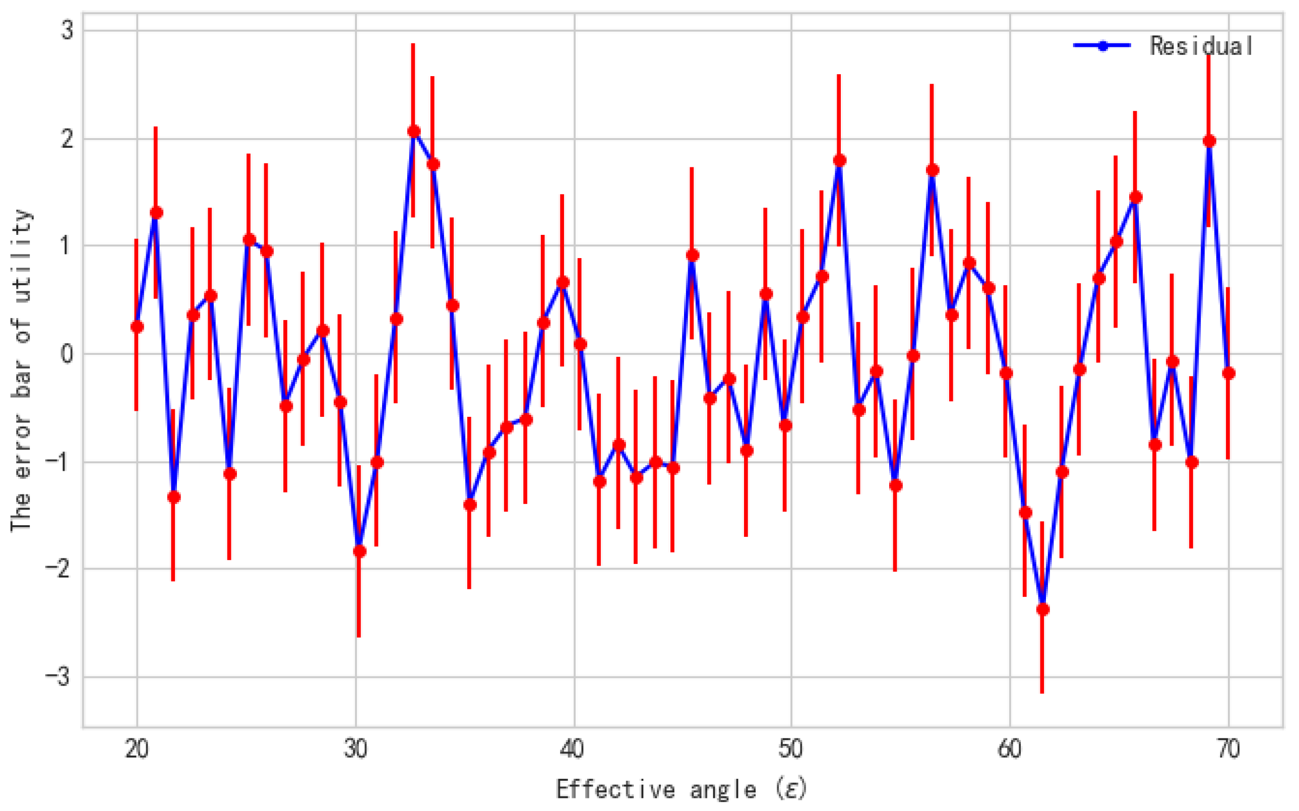
The utility of the original integration method is recorded as $E^{\prime }$, the utility defined in this paper is recorded as E. Then, using one of them as a criterion, the residual is defined as $\mathsf{\Delta }E$, $\mathsf{\Delta }{E}^{\prime }=E^{\prime }-E$. So get a series of point sets, an ordered pair: $({ϵ}_1$, $E_1^{\prime })$, $({ϵ}_2$, $E_2^{\prime })$, $({ϵ}_3$, $E_3^{\prime })$, $({ϵ}_4$, $E_4^{\prime })$, …, and $({ϵ}_1$, $E_1)$, $({ϵ}_2$, $E_2)$, $({ϵ}_3$, $E_3)$, $({ϵ}_4$, $E_4)$, ….

Given a special case, assume that the distribution of $E^{\prime }$ is infinitely close to the E, then $\mathsf{\Delta }E$ is a set of normal distributions approaching the following results can be drawn:

In the normal distribution, $\sigma$ represents the standard deviation and $\mu$ represents the mean. $x=\mu$ is the axis of symmetry of the image. According to the 3$\sigma$ principle [15]:

• The probability distribution in ($\mu -\sigma$, $\mu +\sigma$) is 0.6826.
• The numerical distribution rate is 0.9545.
• The probabilities in the probability distribution ($\mu -2\sigma$, $\mu +2\sigma$) in ($\mu -3s\sigma$, $\mu +3\sigma$) are 0.9973.

It can be assumed that the value of the index is almost entirely within the ($\mu -3\sigma$, $\mu +3\sigma$) interval, and the probability of exceeding this range is only less than 0.3%.

Evaluation Results

According to the normal distribution analysis method in the previous section, the distribution image after determining ${\mu }_1$, $\alpha$ and $\mathsf{\Delta }E$ is shown in Figure 7.

From Figure 7, we can see that the two strategies do not follow the standard normal distribution, and the closer to 0 the smaller the difference, the polyline fluctuations in the vicinity of 0, indicating that the difference between the two strategies is larger.

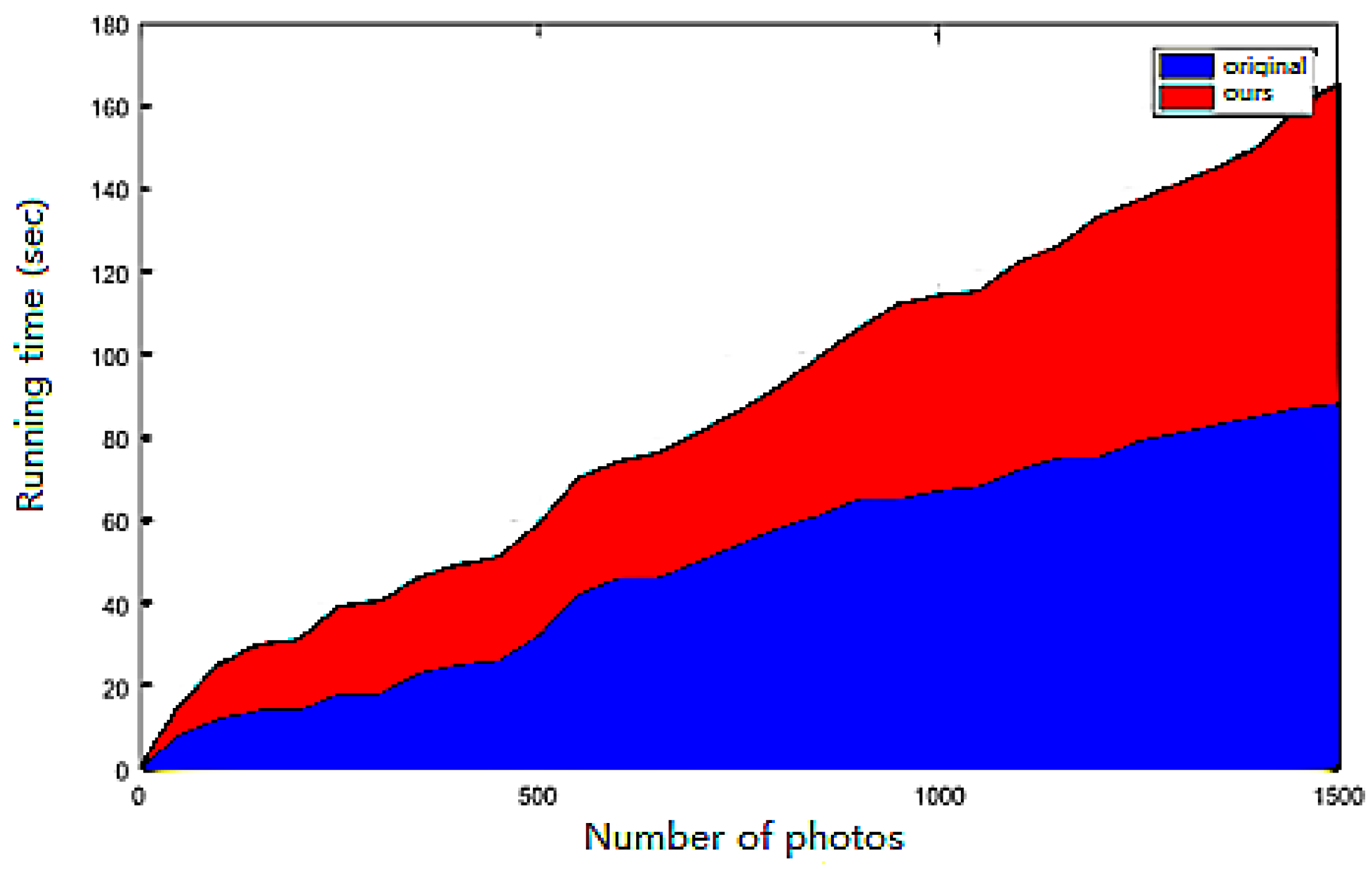
In view of the above two utility computing methods, this paper compares the two factors according to the running time and the CPU occupancy rate in order to prove the effectiveness of the proposed strategy.

Figure 8 illustrates the time comparison between the two strategies when calculating the same number of photo utility. Under the same conditions, the experimental equipment used in this study is shown in

Table 2. Configuration information for the lab device.

Rekated Property Item	Configuration Information	Remarks
Operating system	Windows 10 64 bit	Uses the window system for compatibility with software tools
Running memory	8192 MB RAM	Increased running time
Processor	Intel Core i9-7900X	N/A
Manufacturer	Lenovo	N/A
Hard disk	500 GB	Access to a large number of experimental data

.

By using the two different strategies and comparing the original utility definition and the utility defined in this paper, in the process of selecting 0 to 1500 photos, we can see that there is no significant difference between the original utility and the utility defined in this paper when the number of photos is about 500. After 500, the stack diagram shows that the running time of utility defined in this paper is obviously less than the original utility, indicating that the utility of this paper is more effective than the original in the problem of large scale image selection. In practice, for servers that need to handle large scale image data, the utility computing method defined in this paper can reduce the load of the server and respond to the requests of multiple users in the least time. Therefore, the utility computing method defined in this paper is superior to the original utility computing method.

The same experimental equipment as shown in Table 1, Figure 9 is the comparison of CPU occupancy rate of the two utility strategies, because the experimental program itself will consume a lot of CPU computing resources, so the CPU scheduling algorithm will also affect the program itself. The premise is to use multi-core CPU, so the experimental equipment will inevitably require the use of it to conduct experiments. Under the same circumstances, using the utility computing strategy defined in this paper and the original utility computing strategy in the process of selecting from 0 to 1600 photos, the utility computing strategy defined in this paper is superior to the original utility in the resource utilization of the CPU. This paper shows that the utility of this paper is more reasonable and it is coordinated with the classic scheduling algorithm of the CPU. Such as short-job-first algorithms, first-come-first-service algorithms, round-robin scheduling algorithms, etc. Therefore, in terms of CPU usage, the utility computing strategy defined in this paper can make more reasonable use of computing resources. For servers that need to consume large amounts of computing resources, the utility defined in this paper is more reasonable than the original utility.

4. Minimum Selection Algorithm

In the following description, it is assumed that the coverage requirements of each target can be satisfied by the entire set of photos.

4.1. Problem Conversion

Firstly, transform coverage requirements into coverage requirements acreage. Generally, consider a single target area ${\mathsf{\Gamma }}_i$ and use coverage arc $Q_j=[0,2\pi )$ to represent coverage requirements, As shown in Figure 10. $F=\left\{f_1,f_2,\dots ,f_m\right\}$ denotes the set of all photographs covering ${\mathsf{\Gamma }}_i$, for each $F_j$, if ${\mathsf{\Gamma }}_i$ is covered by $F_j$, then the coverage of $F_j$ (the gray sector in Figure 2) on ${\mathsf{\Gamma }}_i$ can be represented as a sub-arc of $[0,2\pi )$. As shown in Equation (9):

$$I_j=[x_j,y_j]=[arg(\overrightarrow{T_{\mathsf{\Gamma }}{F}_j})-\epsilon ,arg(\overrightarrow{T_{\mathsf{\Gamma }}{F}_j})+\epsilon ]$$

(9)

Here, the two endpoints $x_i,y_i$ called split points divide the arc $Q_j$ into two segments: one is $Q_j$ and the other is $Q_j-I_j$. If there are more photos covering ${\mathsf{\Gamma }}_i$, there would be more split points. The split points corresponding to the m photos divide the arc $Q_j=[0,2\pi )$ into $k(k\le$ 2 m) sub-arcs, and each sub-arc corresponds to a sector $S_I$.

Given a set of k elements $U=\left\{u_1,u_2,\dots ,u_k\right\}$ where each element represents a sector corresponding to a sub-arc and k is their total number. The weight of each element is the acreage of the corresponding arc of the sub-arc. For each photo $F_j$, a subset of U can be generated based on the covered sub-arc. Let $I_j$ denote the subset, then it can figure out the following problem to find the solution of the minimum selection problem:

Giving a universe set $U=\left\{u_1,u_2,\dots ,u_k\right\}$ (non-negative), $I=\left\{I_1,I_2,\dots ,I_j\right\}$ of the corresponding sub-arc for each photo, assuming ${\bigcup }_j^n{I}_j=U$, how to choose a subset $I^{\prime }$ of I so that ${\bigcup }_{I_j\in I^{\prime }}{I}_j=U$ is the minimal.

This is an example of a set coverage problem which has been proven to be NP-hard [16]. Therefore, the approximate algorithm can solve the problem of minimum selection based on greedy selection.

4.2. Minimum Selection Problem Algorithm

More specifically, the algorithm first selects photos that covers the most sub-arcs (elements). Once the photo is selected, the sub-arc that it covers will not be considered. The photos are selected one by one according to how many new sub-arcs can be covered. At each time it selects a photo that covers the most sub-arcs. Quit the selection if all sub-arcs are covered or no more photos can be selected (i.e., the photos are all selected or cannot get more utility). Once it finds the required photos, all the elements in are covered, which means all target coverage requirements are satisfied. By using the similarity argument of Theorem 3.1 in [16], it can be found that the number of selected photos is limited, as the Theorem 1 shows.

Theorem 1.

For the minimum selection problem, the worst time complexity of using greedy algorithm is $O(m^{3}n)$.

Proof. 

The time required for conversion to cover the require acreage is $O(nm+nmlogn)$. In the process of selection, pick up the photo that composes the most number of new elements and complete the selection in any step between 1 and m. Considering the worst case condition, if the algorithm ends in m steps, the number of candidate photos is: $1+2+3+\cdots +m=O(m^3)$. It takes time $O(nm)$ to process each candidate photo, so the time complexity of the entire selection algorithm is: $O(nm+nmlogn+m^{2}nm)=O(m^{3}n)$. The algorithm pseudocode is shown in

Table 3. Algorithm pseudocode.

Input:	The angle of the photos: ${\mathit{F}}_1({\mathit{\theta }}_1),{\mathit{F}}_2({\mathit{\theta }}_2),\mathit{\dots },{\mathit{F}}_{\mathit{m}}({\mathit{\theta }}_{\mathit{m}})$ The related parameters of the camera
Parameter:	Effective angle: ϵ
Step:
1:	For $i\leftarrow 1$ to $i\leftarrow n$ do
2:	//To assign a value to the form of an interval
3:	$F_i\leftarrow F_i({\theta }_i-ϵ,{\theta }_i+ϵ);$
4:	$U\leftarrow F_i$; //Adding the molecular interval to the interval set U
5:	End for
6:	//The partition of the interval
7:	While $u_1$ to $u_k$ do
	//Ergodic interval U
8:	//Merging sequence: $e_1,e_2\dots e_j$;
9:	For $r\leftarrow 1$ to $r\leftarrow j$ do
10:	//In the polar coordinate system, it is transformed into the form of sub intervals of elements through the neighborhood principle.
11:	//Sort, get a new sequence of E
12:	End for
	//End the sortation and return to the ordered sequence E
13:	//Transform into $S_t$ interval cover form
14:	$S_t\left\{e_1^{\prime },e_2^{\prime }\dots e_h^{\prime }\right\}\leftarrow u_h$;
15:	End while
16:	//Traversing the new interval set S to select the most efficient combination of photos.
17:	Repeat
18:	If it contains the most multiple interval then
19:	Add to the final photo set
20:	End if
21:	Until all the elements are traversed
22:	Output the final selection $S_{resultset}$

. ☐

In an emergency circumstance, some crowdsourced images may contain inaccurate information. The photos must be taken in a very short time, and the user does not have much time to think. Even though the data-unit can help users comprehend how and where photos were taken, some factual and helpful photos may still be missed. The reason for the inaccuracy may be due to various problems, such as image blurring because of the shaking of mobile phone, occlusion, chromatic aberration, or even inaccurate acquisition of the data-unit. To decrease the loss of the important aspects of the target area, the minimum selection algorithm requires a certain degree of fault tolerance, which can be achieved by times of coverage.

4.3. k Times Coverage Based on Minimum Seletion

Some crowdsourcing photos may contain inaccurate information. When an emergency occurs, the photo must be taken in a very short time, leaving little time to the user. Even if data-unit helps to understand how photographs are taken, some real photographs may still be missed. For various reasons, such as blurring, occlusion, color shift, or inaccurate metadata in SIM layer [17] caused by telephone vibration, it will lead to inaccuracy. To reduce the possibility of losing important aspects of the object, the application may need a certain degree of fault tolerance, which can be achieved through Times coverage.

In this problem, one aspect of the target needs to be covered by $k(k\ge 2)$ times. Each target area has coverage requirements $D_j=[x_j,y_j],x_j\ge 0,y_j\le 2\pi$ and the selected photos were demand to cover $I_j$ interval k times. The problem can be defined as follows:

Definition 2 (k times coverage).

Given a set of n target areas $\mathsf{\Gamma }=\left\{{\mathsf{\Gamma }}_1,{\mathsf{\Gamma }}_2,\dots ,{\mathsf{\Gamma }}_n\right\}$, a set of m photos $F=\left\{f_1,f_2,\dots ,f_m\right\}$ with known data-unit. Coverage requirements for each target area defined as $D_i=[x_i,y_i]$ with $x_j\ge 0,y_j\le 2\pi$, integer $k\ge 2$. The problem requires a minimum number of photos among candidates so that the coverage requirements for each target is covered at least k times.

Since the initial minimum selection problem can be transformed into a circular arc coverage problem, hence, the k times coverage problem can be converted to the initial multiple-coverage arc problem. As its name suggests, the multi-transformation problem differs from the set-coverage problem that each element u must appear at least k times in the subset of U, where k is a positive integer. The original greedy algorithm based on the minimum selection problem can be extended to k times coverage problems. To be specific, one element is normal until it becomes inactivity after being covered times. In each step of the selection, the photo that covers as many normal elements as possible is preferential, and the normality of the factors contained in this photo is updated. Until all elements are negative (inactivity), or no more photos can be selected (all photos are selected or cannot be obtained). Assume that all photos are selected to meet coverage requirements. Dobson [18] proved that the above algorithm achieves a time complexity of $O(logmn)$ which means that the number of photos selected by the greedy algorithm will not be $O(logmn)$ times more than the minimum number of photos in principle.

4.4. Conclusions

In each step of the greedy algorithm, for each photo, it counts the number of elements whose aliveness value would decrease if the photo were selected. Then it picks the photo with the largest count, and update the aliveness values accordingly. Here the decrease of an aliveness value means previously alive = 2 and after selecting the photo alive = 1, or previously alive = 1 and after selecting the photo alive = 0. This selection process continues until all alive = 0 or no more photo can be selected (either photos are all selected or no more benefit can be achieved). The performance of the greedy algorithm will be evaluated in Section 5.4.

5. Scene Experiment and Simulation

5.1. Data-Unit Acquisition

This research uses a mobile device with Android 7.1.1 system to capture data-unit and record it on the phone automatically. The position information is obtained by using GPS module and calculated based on messages from the Inertial Measurement Unit (IMU) [19,20,21]. Error analysis will be presented in the next section. The field of view $\lambda =2arctan(\frac{w}{2f})$, where w is the width of the image sensor and f is the focal length, both of which can obtained from the Android API [22,23,24]. During the experiment, all photos have the same field of view. Finally, the acquisition of the effective range of mobile phone is more complex which can be affected by many practical factors such as focal length, camera quality, and application requirements. Different applications may use different effective ranges depending on whether observe the occluded objects or accept distant photos [25,26,27].

Direction is also a critical factor. The method used to characterize position in the Android system is to define a local coordinate system, a global coordinate system and a rotation matrix. The rotation matrix is used to convert local coordinate tuples to a global one. Another way to represent a rotation matrix is to use a triplet that includes azimuth, pitch, and roll, representing the rotation of the mobile device around the x, y and z axes respectively [26].

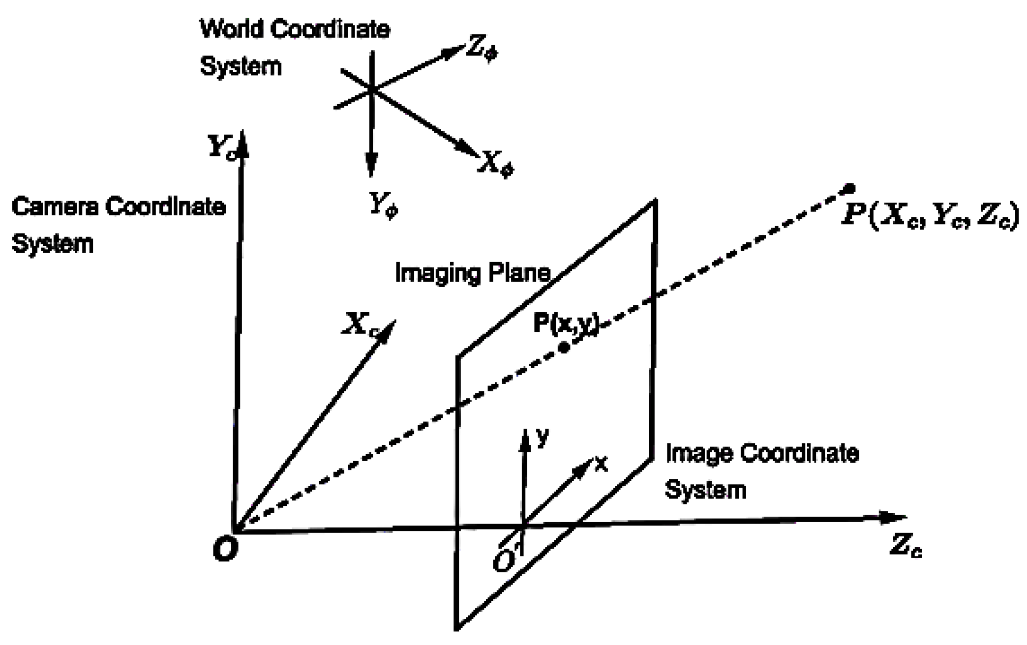
$\alpha$ and $\beta$ are determined by the camera coordinate system at the two ends of the target segment, and the camera imaging geometric relationship can be represented by Figure 11 where O is called the camera optical center and the x-axis and y-axis are parallel to the x-axis and y-axis of the imaging plane coordinate system. The z-axis is the optical axis of the camera and is perpendicular to the image plane. The intersection of the optical axis and the image plane is the image principal point $O^{\prime }$, and the orthogonal coordinate system consisting of the point O and the x, y, z-axis is called a camera coordinate system. $O{O}^{\prime }$ is the focal length.

In a certain environment, the world coordinate system [28,29] is commonly used to describe the position of the camera and the object. The relationship between the camera coordinate system and the world coordinate system can be described by a rotation matrix and a translation vector. Thus, the homogeneous coordinates of a point in the world coordinate system and the camera coordinate system are respectively sum and exist as follows:

$$\left[\begin{array}{c}{X}_C\\ Y_C\\ Z_C\\ 1\end{array}\right]=\left[\begin{array}{cc}R& t\\ 0^r& 1\end{array}\right]\left[\begin{array}{c}{X}_W\\ Y_W\\ Z_W\\ 1\end{array}\right]=M_1\left[\begin{array}{c}{X}_W\\ Y_W\\ Z_W\\ 1\end{array}\right]$$

(10)

where $X_C,Y_C,Z_C$ represent the camera coordinate system, $X_W,Y_W,Z_W$ represent the world coordinate system [30,31].

In this experiment, the reference range is 100 m and the coverage requirements are defined from $0^{\circ }$ to ${360}^{\circ }$.

5.2. Occlusion and out of Focus

In the android system, the rotation matrix can be obtained directly from the accelerometer [32] and magnetic field sensor readings [33,34]. The accelerometer measures the appropriate acceleration of the three axes of the mobile phone in the local coordinate system, including the influence of gravity. The magnetic field sensor provides readings of the surrounding magnetic field along three axes in a local coordinate system. The coordinates of the geocentric coordinates and the surrounding magnetic field are known in the world coordinate system. Therefore, by combining the above readings, the direction of photographing can be obtained.

Assume that most of users will check whether the object appears in the photo after shooting visually. However, if the user does not check the photo and the object is hidden by an unexpected obstacle such as a moving vehicle, the photograph is invalid for the server. Even if the user checks the photo and the object is clear, it may be different from what the server expects. For example, the server may expect the photo to be related to a building, but the user may be looking at a tree in front of the building. Although in both cases, the smartphone can produce the same data-unit, the content may not be the same. In addition to this issue, targets may be out of focus in many other situations. Uploading these photos will waste a lot of bandwidth and storage space.

The application uses a function called focus distance [26], and many smartphones with focusing capabilities can provide this functionality. The focus distance is the distance between the camera and the object that is perfectly focused on the photo. The actual distance between cameras and people’s interested targets can be calculated by GPS location. Therefore, ideally, if the two distances do not match, the target is out of focus and the photo should be excluded.

The error in measuring the focus distance is relatively large. A slight offset does not mean that the goal is not concentrated. In reality, the distance between the closest and farthest objects in a photograph is acceptable which called the depth of field (DOF).

Depth of field is affected by four parameters: focal length (f), focus distance (d), lens aperture (A), circle of confusion. Among these parameters, focal length (f) and lens aperture (A) are acquired from the Android API. Circle of confusion has a pre-defined value that determines the resolution limit of the application. Focus distance (d) is also available in the API and not the same in each instance. So it can calculate the DOF by: $D_{near}=v_0(H-f)/H+v_0-2f$, $D_{far}=v_0(H-f)/H-v_0$. According to [26], $H=\frac{f^2}{k\times E}$, where H is a hyperfocal distance.

After the photo is taken, the system compares the distance between the target and the camera to the above two values. If the target falls into the depth of field, the photo is considered valid; otherwise, it will be excluded. This filtering is done on the client side. Data-unit for unqualified photos will not sent to the server.

5.3. Scenario Testing

The experiment verifies the effectiveness of the proposed photo selection algorithm by implementing real-world scene experiments. The cast is the target of this experiment, and the mobile device is able to record the data-unit automatically after reprogramming, and then all the data-unit of the photos are uploaded to a central server. In this test, we took 40 photographs of the function. Most of the photographs were taken around the target statue. Some of the photographs were taken directly to the target statue and some were not. In fact, people are more inclined to shoot in the front of the target, in order to simulate the actual situation, the number of photos at different angles in the experiment is different, based on three different algorithms:

• Minimum selection algorithm.
• Random Algorithm 1 based on position: select the candidate photos randomly.
• Random Algorithm 2: random selection in candidate photo sets.

The minimum selection algorithm selects six photos to meet the coverage requirements as shown in Figure 12a. The angle between any two adjacent observation directions (connecting the camera and the dotted line of the target) is less than 80 degrees. Because the effective angle is set to 40 degrees. Compared with the minimum selection algorithm, as shown in Figure 12b, the location-based random selection algorithm1 selects the photos one by one randomly until the coverage is achieved. It selects at least 13 photos to meet the same coverage requirements as shown in Figure 12b. The random selection algorithm 2 selects the number of photos as 20, as shown in Figure 12c. The experiment is repeated 100 times, and an average of 25 photographs can be selected each time to satisfy the same coverage requirements.

The random algorithm chooses at least 15 photos to meet the same coverage needs. Experiments based on the random selection algorithm were repeated 100 times, and an average of 21 photos were selected to meet the same coverage requirement. This shows that the minimum selection algorithm reduces the number of selected photos to achieve the desired coverage significantly.

The above data shows that under the same coverage requirements, the minimum selection algorithm significantly reduces the number of selected photos to achieve the desired coverage compared to the other two random algorithms.

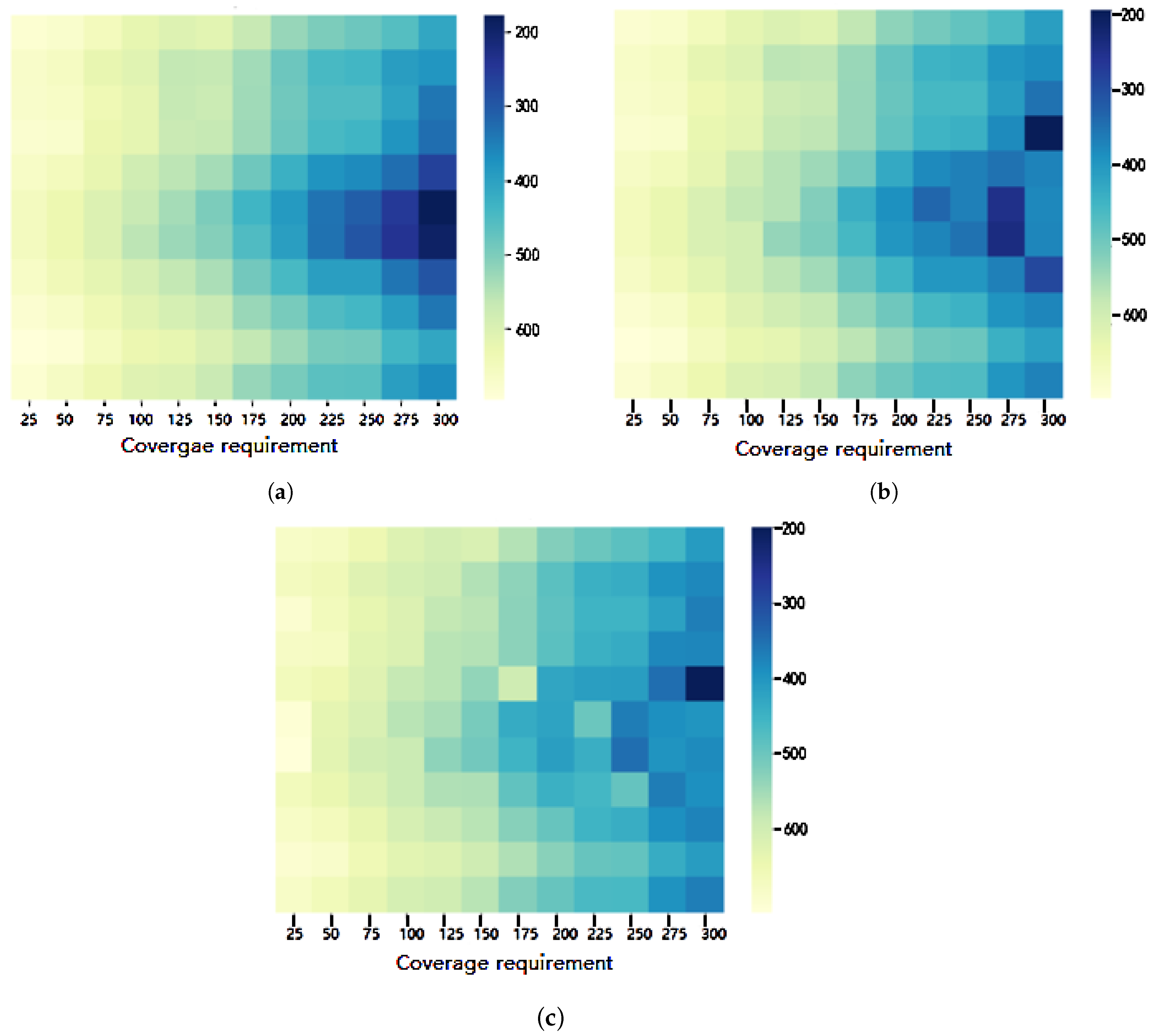
As further illustrated in Figure 13, in the case where the number of candidate photos is increased by 144, a 12 × 12 matrix is formed, and how the three algorithms cover the target area in the same coverage requirements interval. For convenience, the darker the color, the fewer photos are selected. It can be clearly seen from figures that under a certain coverage requirement, the number of photos selected by the minimum selection algorithm (Figure 13a) is the smallest, followed by the random Algorithm 1 (Figure 13b), and the number of photos selected by the random Algorithm 2 (Figure 13c) is the largest. The above proves the practical effectiveness of the minimum selection algorithm in this paper.

5.4. Simulation Experiment

In this section, we evaluate the photo selection algorithm by simulation. The targets are distributed within a 100 × 100 m square meter area randomly. The photos are evenly distributed over a 200 × 200 m square meter area where the target area is in the center and shooting direction is distributed from 0 to 2$\pi$ randomly.

The field of view of the camera is set to ${120}^{\circ }$. In the simulation process, the minimum selection algorithm is compared with the random selection Algorithm 1 and the random Algorithm 2. It compares the random selection algorithm with minimum selection algorithm which selects photos at each step randomly until the coverage requirements are satisfied. For an impartial comparison, it only considers photos that cover at least one target which is called related photos.

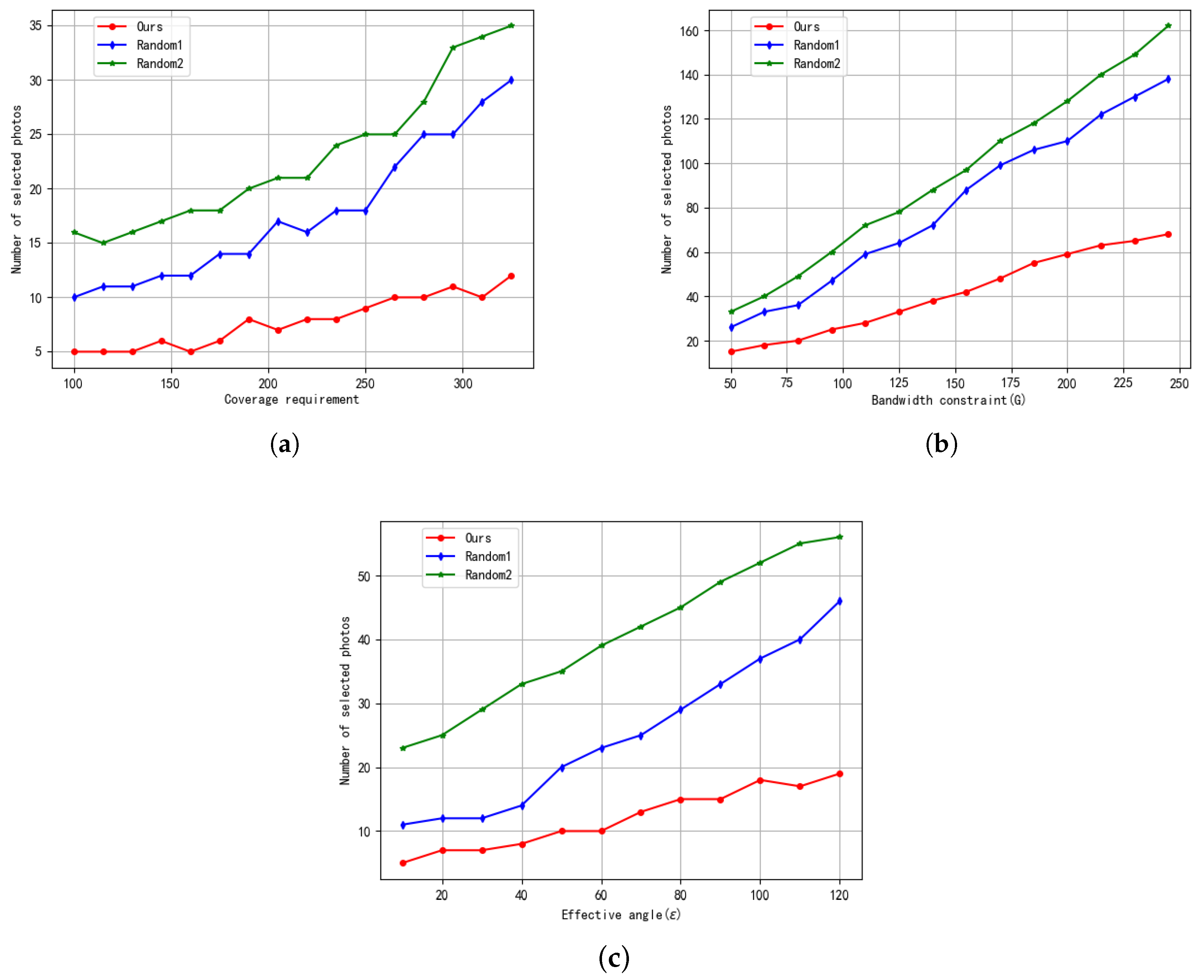
Figure 14 shows the comparison of the effectiveness of the three selection algorithms by changing three parameters: coverage requirement, bandwidth limitation, and effective angle. Figure 14a shows that when the bandwidth $G=125$ M and the effective angle $ϵ={60}^{\circ }$, it can be clearly seen that the number of photos selected by the random algorithm is higher than the minimum selection algorithm when initially selected. With the increase of coverage requirements, the number of photos selected by the minimum selection algorithm is growing slowly and is lower than the other two algorithms.

Figure 14b shows that when the effective angle $ϵ={60}^{\circ }$ and the coverage requirements $I={128}^{\circ }$, the number of photos selected by the three algorithms grows as the bandwidth increases, but the growth rate of the minimum selection algorithm is slow, when it reaches a certain bandwidth limitation, it will not grow again, but stabilize at a certain value.

Figure 14c shows the changing trend of the three selection algorithms in the case where the bandwidth $G=125$ M and the coverage requirements $I={128}^{\circ }$, the effective angle is changed. It can be clearly seen that the minimum selection is better than the other two random algorithms.

5.4.1. Simulation Results of Minimum Selection Algorithm

In fact, the given pool of photos might be very large, and as the number of photographs increased, the number of related photos also increased. Figure 15a shows the effectiveness of the minimum selection algorithm in reducing redundancy. There are 20 targets that demand covering all angles from $0^{\circ }$ to ${360}^{\circ }$. Since the total number of photos varies from 300 to 1500, the number of related photos increases linearly. Nevertheless, the number of photos selected by minimum selection algorithm does not increase. It reduces slightly since the minimum selection algorithm makes use of the increased density of photos to improve efficiency.

In the case where the number of targets (n) varies from 5 to 50, the total number of photos is fixed at 500, and all other factors remain unchanged. As shown in Figure 15b, the algorithm must choose more photos to cover more targets. However, the number of photos selected by the minimum selection algorithm is very small, the growth rate is much slower as the number of target increases, which is obviously more effective than the random algorithm.

In Figure 15c, we fix the number of targets to 20 and change the number of aspects that need to be covered on each target. As one would expect, as the aspect increases, the number of photos that reach the demand for coverage also increases. The minimum selection algorithm selects photos that satisfy the coverage requirements significantly less than the random algorithm. Therefore, the effectiveness of the minimum selection algorithm is verified.

5.4.2. k-Coverage Simulation Results

In this section, we discuss the minimum selection of times coverage by comparing three models, which are 1, 2, and 3, respectively. As shown in Figure 16a, the number of selected photos is a function of the total number of photos, other parameters are fixed. All algorithms are able to make effective selection as the increase in the total number of photos. Comparing 1 times coverage, 2 times coverage and 3 times coverage, the number of selected photos is almost proportional to the coverage (k). It shows that there is no difference between the single coverage and the k times coverage which just repeat the single coverage for k times.

In Figure 16b, the number of targets is changed from 5 to 50 while the total number of photos is fixed at 1000. For the target, all angles from $0^{\circ }$ to ${360}^{\circ }$ should meet the coverage requirement level. The relationship between the bar charts is similar to the transformation in Figure 15a, and the trend is similar to that in Figure 15b. In Figure 16c, the total number of targets is remaining constant, then it changes the number of coverage aspect requirements. The relationship between the bar transforms is similar to Figure 16a,b, and the increasing trend of bar charts is similar to that in Figure 15c.

6. Accuracy Analysis

6.1. GPS Acquisition

A study in 2011 shows that the median error in the GPS module of smart phones is 5 m–8.5 m [35], which is very small compared to the size of the photograph or the size of the target area. With the continuous development of GPS technology and improvement in precision [29], it is expected that the latest mobile devices will have even smaller errors. For the acquisition of directions, three IMU sensors (accelerometers, magnetometers, gyroscopes) are used, and the average error can be reached ${1.3}^{\circ }–{3.4}^{\circ }$ [21,36]. The authors also found that new devices with more advanced hardware and operating systems are more accurate. Therefore, in the design of this paper, position and orientation errors are negligible.

6.2. Occlusion Problems

Obstruction means that the target is blocked by an obstacle. Although the coverage is based on the data-unit, all the content behind the obstacle is not visible in the photo, and the coverage of the photo should be changed accordingly. The coverage area may no longer be a circular sector and could be any form depending on the position and shape of the obstacle. Unless processing the content of the image itself, occlusion is more difficult to detect and requires a lot of computing resources. If occlusion causes the subject to focus [37], the camera’s parametric depth of field can be used to detect occlusion. However, when the targets and obstacles are very close to each other, the depth of field cannot be detected. Another method is to check the map. Meanwhile, take advantage of the location and shape of the building to test the block caused by the building. This idea needs further research because it cannot detect the obstruction caused by other obstacles such as trees or vehicles. Due to its complexity, research will continue to be down in the future. It should be noted that the occlusion issue is not inconsistent with the content of this paper. The design of this paper applies to any shape of coverage area. If it solves the occlusion problem and finds a more accurate coverage area, it can improve performance. For the current study, a fan-shaped model can be used, which represents the general situation and work well in experiments. At the same time, the utility measure of this paper covers the target area from multiple aspects, effectively reducing the occlusion problem.

6.3. Images Quality Control

Due to several issues such as blurring, distortion, noise, and inappropriate brightness, there are some low quality problems in crowdsourced images. Collecting and analyzing the limited resources of these photos. Therefore, before the data-unit is sent to the server, image quality assessment (IQA) [31] can be used on the mobile device to detect the quality of the photo. The data-unit of low quality photos will not be sent to the server. However, the existing image processing technology calculations consume a lot of resources that the resource limitations of mobile devices should be taken into account in order to make adjustments.

7. Summary

This paper proposes a crowdsourcing image selection algorithm based on data-unit. The algorithm forms a model by acquiring the data-unit of photos taken by the smart device which including GPS position, direction, etc. The data-unit is smaller than the pixels of the image. Therefore, in the application scenario where resources such as bandwidth, storage, computing capacity, and device quality are severely limited, the smart terminal device can efficiently send data-unit to the central server. The server then runs the photo selection algorithm proposed in this paper for all photos to make effective assessments and choices. In addition, this paper suggests to use the effective angle range of the photo to quantify the coverage of target area. The minimum selection algorithm was optimized and proved theoretically. Finally, a simulation experiment was designed and implemented to verify the effectiveness of the above algorithm.

Research in the future:

• Analyzing the information of photos and assigning different weights to them to make further selections. For example: If there are more survivors in a building during an emergency, such as a teaching building where exits obtained by photos should be selected preferably.
• Improving algorithm to eliminate redundancy of images, increasing the accuracy of collecting data-units and mitigating obstacle obstruction and out-of-focus issues.
• The computational efficiency of the algorithm could be enhanced, and take implementing the algorithm in a distributed computing way into consideration.