Joint Adaptive Coding and Reversible Data Hiding for AMBTC Compressed Images


Abstract
:1. Introduction
2. Related Works
2.1. AMBTC Compression Technique
2.2. Hong et al.’s Method
3. Proposed Method
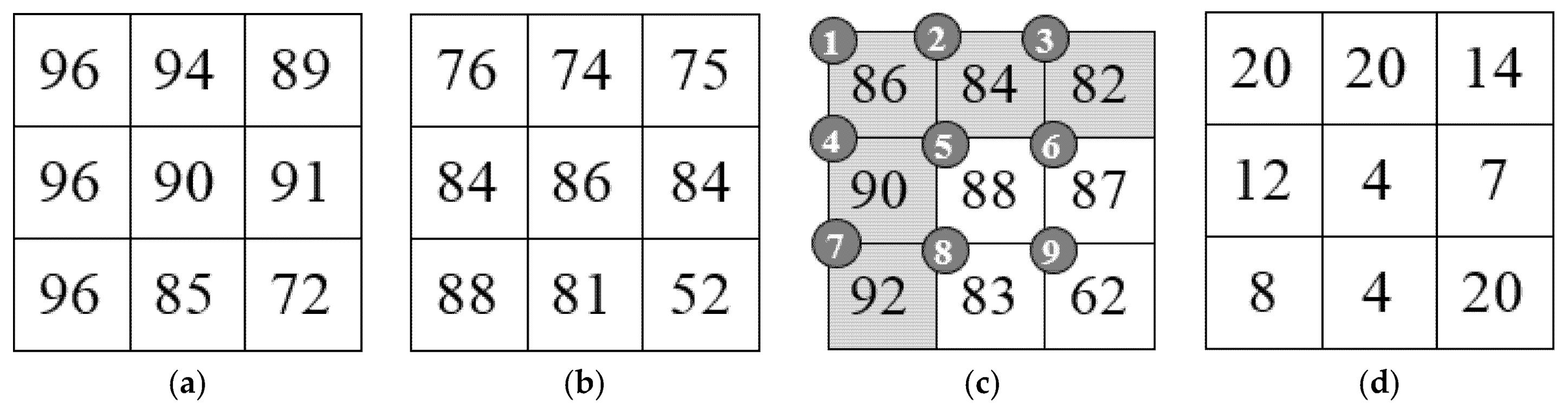
3.1. Reversible Integer Transform of Quantization Levels
3.2. Adaptive Case Classification Technique
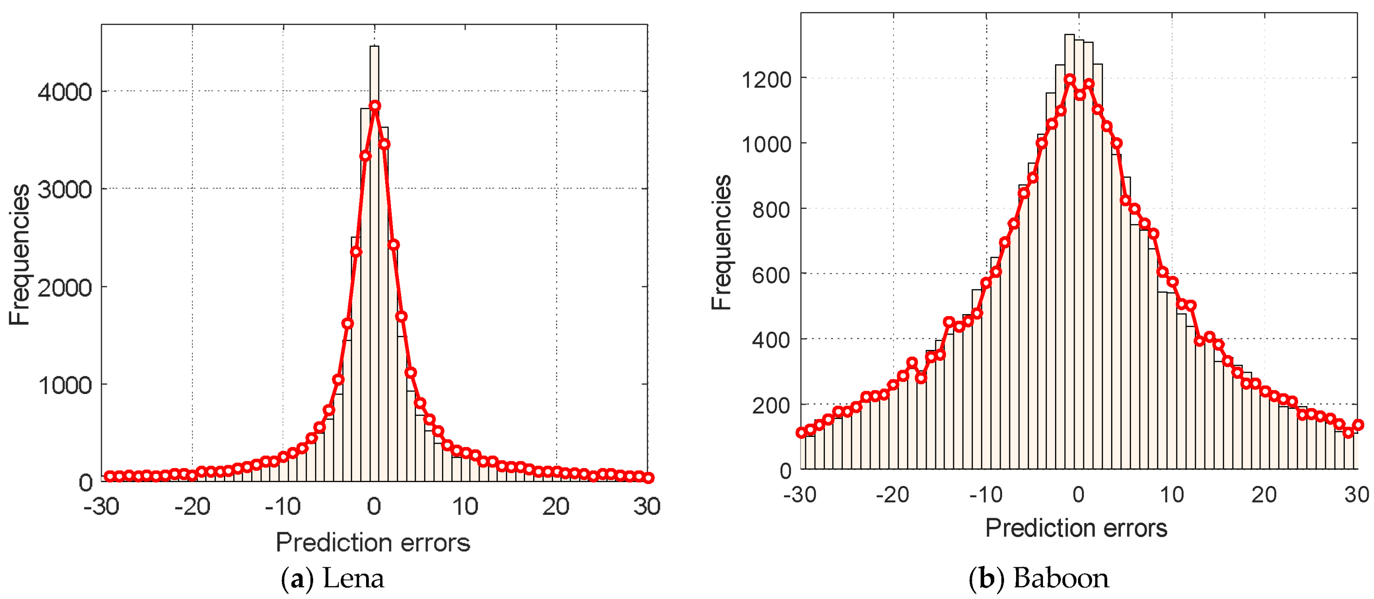
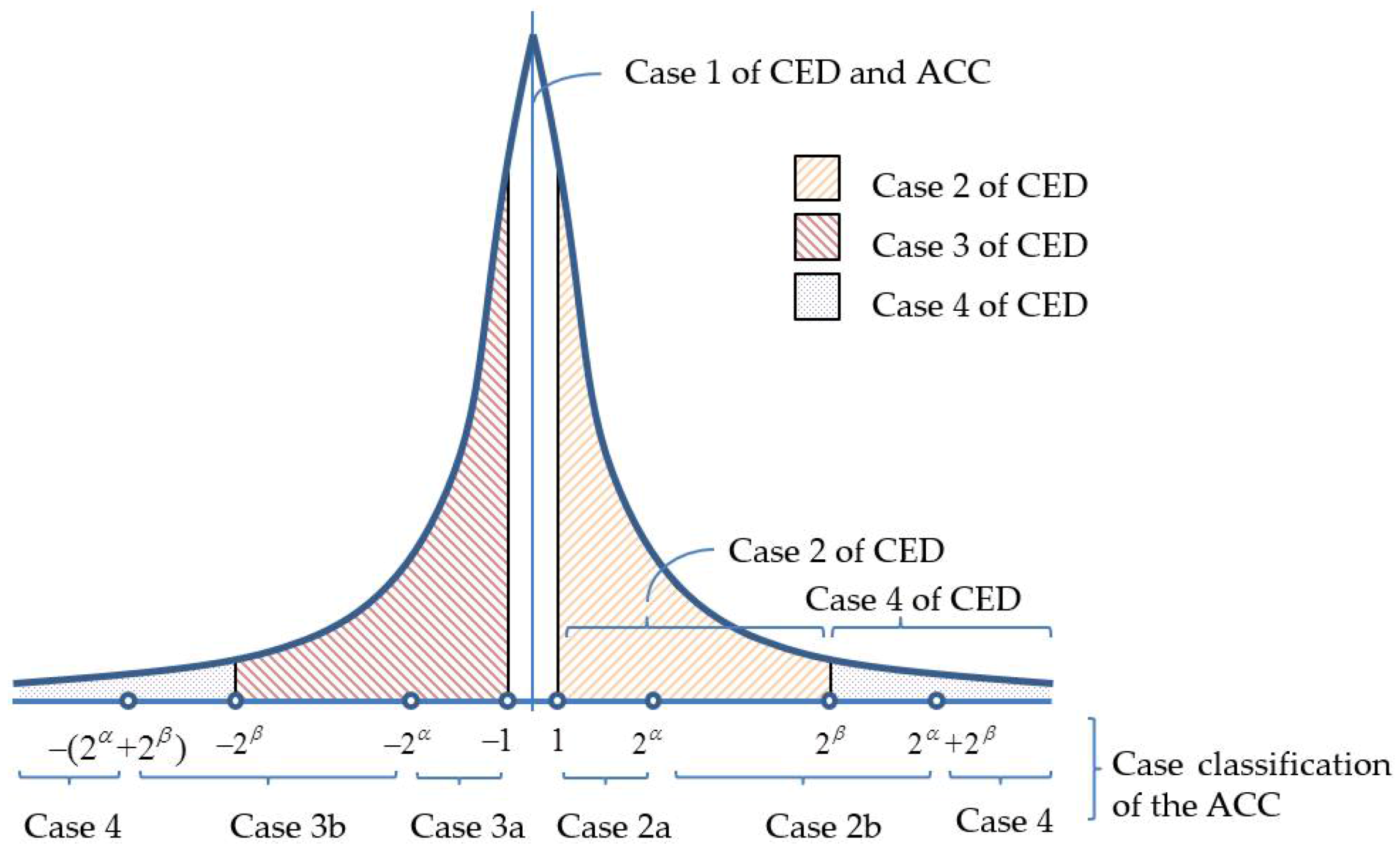
 and each requires bits to record its value. However, the occurring frequencies of prediction errors in the range of vary significantly. Within this range, the occurring frequency is the highest at , in general, and decreases exponentially towards . Therefore, the recording of prediction errors using bits in this range with unbalanced frequencies is likely to increase the bitrate. The encoding of case 3 prediction errors, used in [18], also had similar problems.
3.3. The Embedding Procedures
- Step 1:
- Transform the quantization levels, and , into means, , and differences, , using the RIT technique, as described in Section 3.1.
- Step 2:
- Visit and sequentially, and use the ACC technique described in Section 3.2 to find the best and values, such that the estimated code length is minimal.
- Step 3:
- Convert the elements in the first row and the first columns of and to their eight-bit binary representations. The converted results are appended to the CS.
- Step 4:
- Scan the rest elements in using the raster scanning order and use the MED predictor (Equation (1)) to predict scanned . Let be the prediction value and calculate the prediction error .
- Step 5:
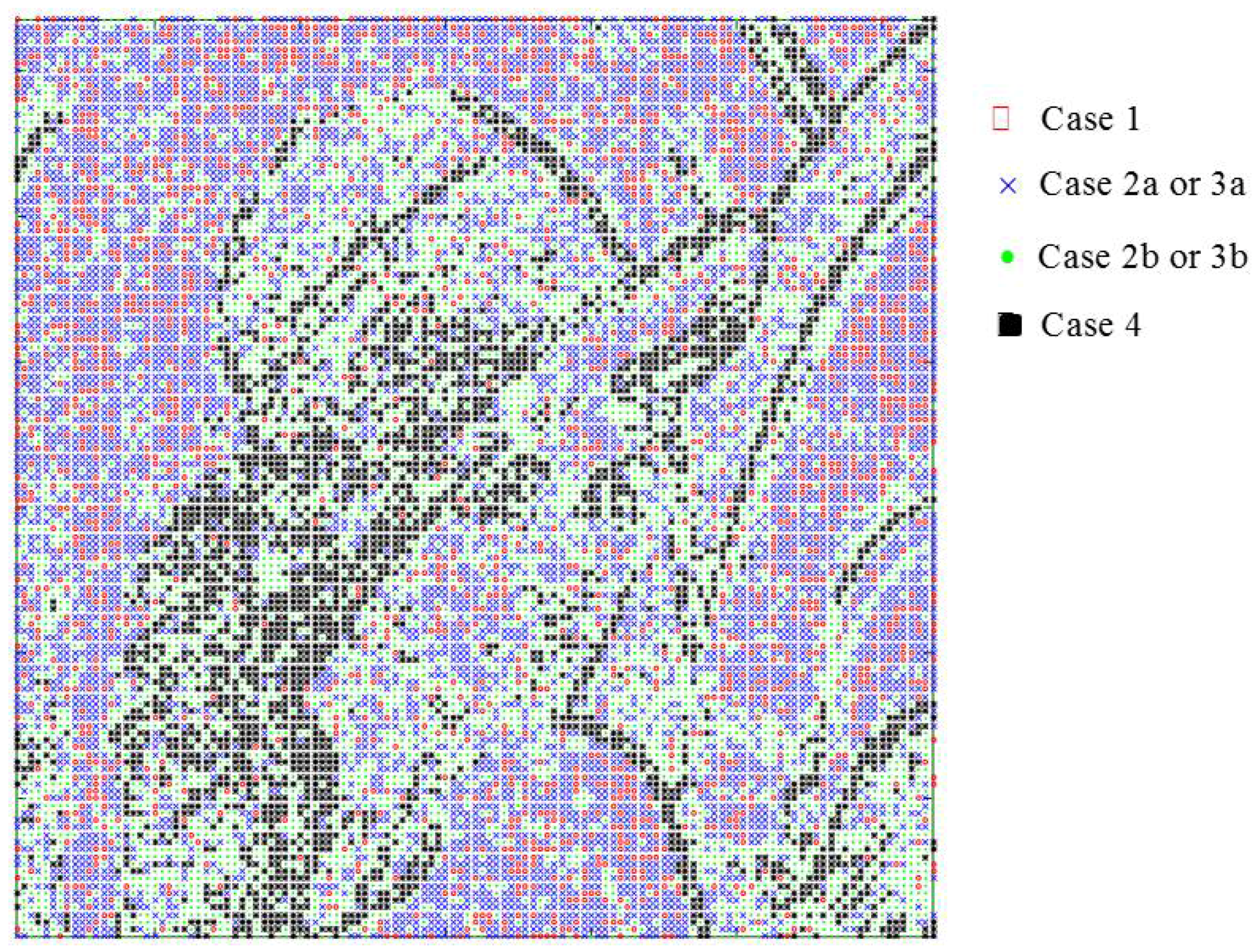
- Extract n-bit secret data, , from S. In accordance with , one of the four encoding cases is applied:
- Case 1:
- If , the bits ||00 are append to the code stream, CS.
- Case 2:
- If , append the bits, ||010||, to the CS, where is the binary representation of y. If , append ||011|| to the CS.
- Case 3:
- If , append the bits, ||100||, to the CS. If , append ||101|| to the CS.
- Case 4:
- If or , append the bits, ||11||, to the CS.
- Step 6:
- Repeat Steps 4–5 until all means, , are encoded.
- Step 7:
- Use the same procedures listed in Steps 4–6 to encode the differences, , and append the encoded result to the CS.
- Step 8:
- Append the bitmap, , to the CS, to construct the final code stream, .
3.4. The Extraction and Recovery Procedures
- Step 1:
- Prepare empty arrays , , , , and S for storing the reconstructed lower quantization levels, upper quantization levels, means, differences, and secret data, respectively.
- Step 2:
- Read eight bits sequentially from and convert them into integers. Place the converted integers in the first row and the first column of .
- Step 3:
- Read the next n bits from and append them to S.
- Step 4:
- Visit the unrecovered means, , in using the raster scanning order. Use Equation (1) to predict , and obtain the prediction value, .
- Step 5:
- Read the next two bits, , from , and use the following rules to recover :
- Case 1:
- If ‘00’, .
- Case 2:
- If ‘01’, read the next bit, , from . If = ‘0’, read the next bits, , from . The mean, , is recovered by , where represents the decimal value of bitstream y. If = ‘1’, read the next bits from . The mean, , is recovered.
- Case 3:
- If ‘10’, read the next bit, , from . If = ‘0’, read the next bits, , from . The mean, , is recovered by . If = ‘1’, read the next bits, , from . The mean, , is recovered.
- Case 4:
- If = ‘11’, read the next eight bits from , and the mean,, is recovered.
- Step 6:
- Perform Steps 3–5 until all the means are recovered.
- Step 7:
- Recover the differences and extract data bits embedded in . The procedures are similar to Steps 2–6.
- Step 8:
- Extract the remaining bits in and rearrange them to obtain . Transform and into and using Equation (3); the original AMBTC codes, , can be reconstructed.
4. Experimental Results
4.1. Performance Evaluation of the Proposed Method
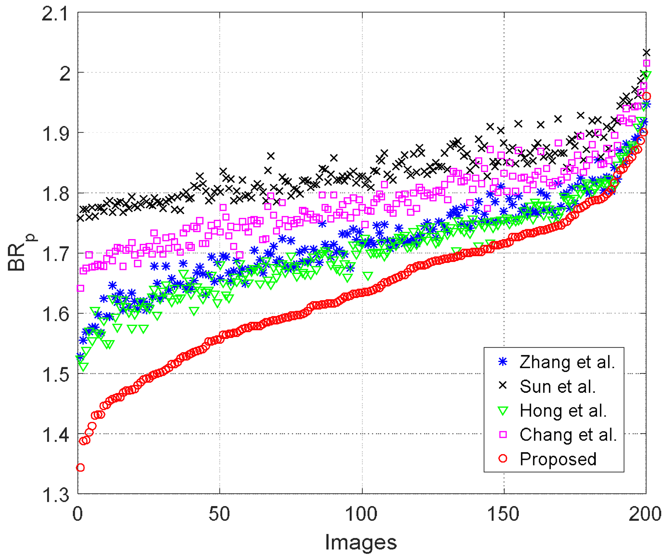
4.2. Comparison with Other Works
5. Conclusions
Author Contributions
Acknowledgments
Conflicts of Interest
References
- Hong, W.; Chen, T.S. A Novel Data Embedding Method Using Adaptive Pixel Pair Matching. IEEE Trans. Inf. Forensics Secur. 2012, 7, 176–184. [Google Scholar] [CrossRef]
- Liu, Y.; Chang, C.C.; Huang, P.C.; Hsu, C.Y. Efficient Information Hiding Based on Theory of Numbers. Symmetry 2018, 10, 19. [Google Scholar] [CrossRef]
- Xie, X.Z.; Lin, C.C.; Chang, C.C. Data Hiding Based on A Two-Layer Turtle Shell Matrix. Symmetry 2018, 13, 47. [Google Scholar] [CrossRef]
- Hong, W.; Chen, T.S.; Chen, J. Reversible Data Hiding Using Delaunay Triangulation and Selective Embedment. Inf. Sci. 2015, 308, 140–154. [Google Scholar] [CrossRef]
- Chen, J. A PVD-Based Data Hiding Method with Histogram Preserving Using Pixel Pair Matching. Signal Process. Image Commun. 2014, 29, 375–384. [Google Scholar] [CrossRef]
- Chen, H.; Ni, J.; Hong, W.; Chen, T.S. High-Fidelity Reversible Data Hiding Using Directionally-Enclosed Prediction. IEEE Signal Process. Lett. 2017, 24, 574–578. [Google Scholar] [CrossRef]
- Lee, C.F.; Weng, C.Y.; Chen, K.C. An Efficient Reversible Data Hiding with Reduplicated Exploiting Modification Direction Using Image Interpolation and Edge Detection. Multimedia Tools Appl. 2017, 76, 9993–10016. [Google Scholar] [CrossRef]
- Tian, J. Reversible Data Embedding Using a Difference Expansion. IEEE Trans. Circuits Syst. Video Technol. 2003, 13, 890–896. [Google Scholar] [CrossRef]
- Ni, Z.; Shi, Y.Q.; Ansari, N.; Su, W. Reversible Data Hiding. IEEE Trans. Circuits Syst. Video Technol. 2006, 16, 354–362. [Google Scholar]
- Chen, J.; Hong, W.; Chen, T.S.; Shiu, C.W. Steganography for BTC Compressed Images Using No Distortion Technique. Image Sci. J. 2010, 58, 177–185. [Google Scholar] [CrossRef]
- Chang, C.C.; Kieu, T.D.; Wu, W.C. A Lossless Data Embedding Technique by Joint Neighboring Coding. Pattern Recognit. 2009, 42, 1597–1603. [Google Scholar] [CrossRef]
- Kieu, D.; Rudder, A. A Reversible Steganographic Scheme for VQ Indices Based on Joint Neighboring and Predictive Coding. Multimedia Tools Appl. 2016, 75, 13705–13731. [Google Scholar] [CrossRef]
- Lin, C.C.; Liu, X.L.; Yuan, S.M. Reversible Data Hiding for VQ-Compressed Images Based on Search-Order Coding and Sate-Codebook Mapping. Inf. Sci. 2015, 293, 314–326. [Google Scholar] [CrossRef]
- Chang, C.C.; Liu, X.L.; Lin, C.C.; Yuan, S.M. A High-Payload Reversible Data Hiding Scheme Based on Histogram Modification in JPEG Bitstream. Imaging Sci. J. 2016, 7, 364–373. [Google Scholar]
- Hong, W. Efficient Data Hiding Based on Block Truncation Coding Using Pixel Pair Matching Technique. Symmetry 2018, 10, 36. [Google Scholar] [CrossRef]
- Zhang, Y.; Guo, S.Z.; Lu, Z.M.; Luo, H. Reversible Data Hiding for BTC-Compressed Images Based on Lossless Coding of Mean Tables. IEICE Trans. Commun. 2013, 96, 624–631. [Google Scholar] [CrossRef]
- Sun, W.; Lu, Z.M.; Wen, Y.C.; Yu, F.X.; Shen, R.J. High Performance Reversible Data Hiding for Block Truncation Coding Compressed Images. Signal Image Video Process. 2013, 7, 297–306. [Google Scholar] [CrossRef]
- Hong, W.; Ma, Y.; Wu, H.C.; Chen, T.S. An Efficient Reversible Data Hiding Method for AMBTC Compressed Images. Multimedia Tools Appl. 2017, 76, 5441–5460. [Google Scholar] [CrossRef]
- Chang, C.C.; Chen, T.S.; Wang, Y.K.; Liu, Y. A Reversible Data Hiding Scheme Based on Absolute Moment Block Truncation Coding Compression Using Exclusive OR Operator. Multimedia Tools Appl. 2018, 77, 9039–9053. [Google Scholar] [CrossRef]
- Lema, M.; Mitchell, O. Absolute Moment Block Truncation Coding and Its Application to Color Image. IEEE Trans. Commun. 1984, 32, 1148–1157. [Google Scholar] [CrossRef]
- Hong, W.; Chen, M.; Chen, T.S.; Huang, C.C. An Efficient Authentication Method for AMBTC Compressed Images Using Adaptive Pixel Pair Matching. Multimedia Tools Appl. 2018, 77, 4677–4695. [Google Scholar] [CrossRef]
- Chen, T.H.; Chang, T.C. On The Security of A BTC-Based-Compression Image Authentication Scheme. Multimedia Tools Appl. 2017, 77, 12979–12989. [Google Scholar] [CrossRef]
- Malik, A.; Sikka, G.; Verma, H.K. An AMBTC Compression Based Data Hiding Scheme Using Pixel Value Adjusting Strategy. Multidimensional Syst. Signal Process. 2017, 1–18. [Google Scholar] [CrossRef]
- The USC-SIPI Image Database. Available online: http://sipi.usc.edu/database (accessed on 29 March 2018).
- BOWS-2 Image Database. Available online: http://bows2.gipsa-lab.inpg.fr (accessed on 29 March 2018).


| Case | Indicator | Range of Prediction Errors | Code Length | |
|---|---|---|---|---|
| case 1 | ‘00’ | 2 | ||
| case 2 | case 2a | ‘010’ | ||
| case 2b | ‘011’ | |||
| case 3 | case 3a | ‘100’ | ||
| case 3b | ‘101’ | |||
| case 4 | ‘11’ | or | ||
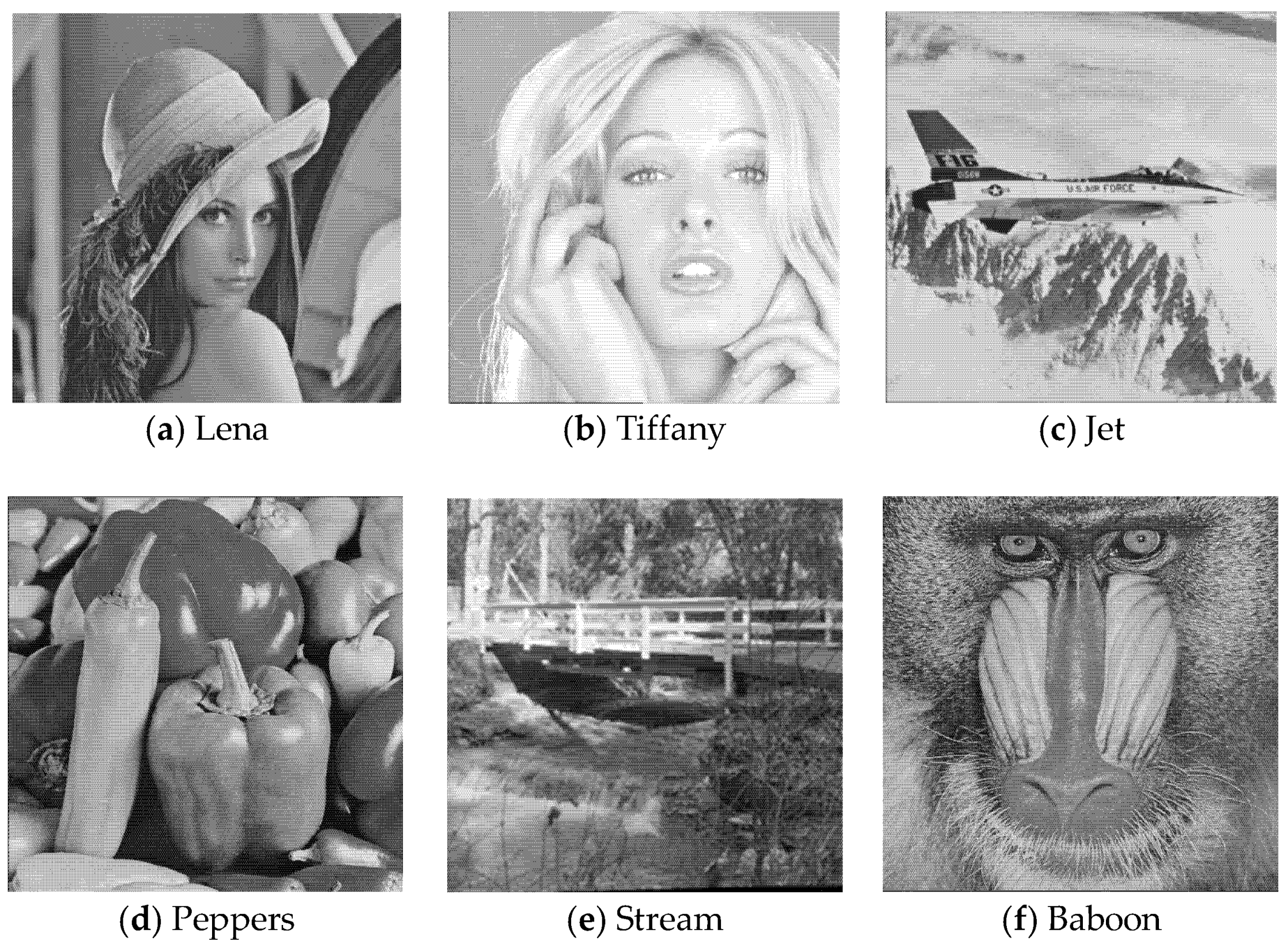
| Images | Lena | Tiffany | Jet | Peppers | Stream | Baboon |
|---|---|---|---|---|---|---|
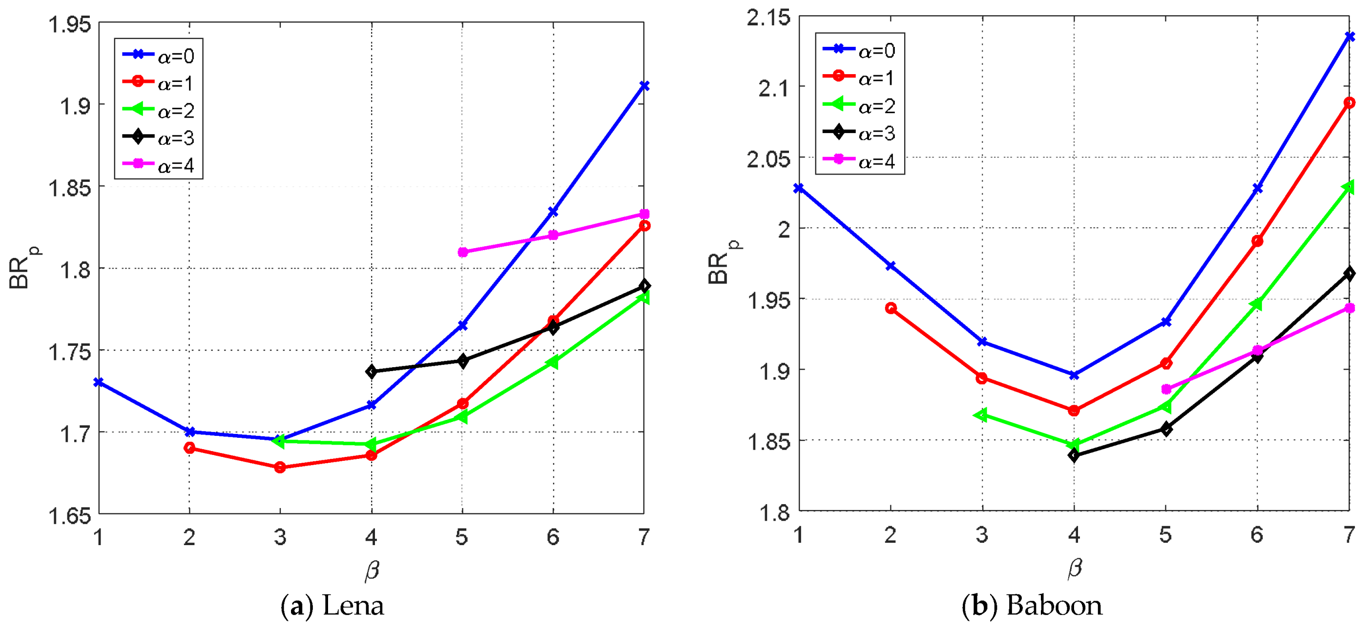
| (1,3) | (1,3) | (1,3) | (1,3) | (3,4) | (3,4) | |
| 1.68 | 1.64 | 1.67 | 1.68 | 1.83 | 1.84 |
| Metric | Methods | Lena | Tiffany | Jet | Peppers | Stream | Baboon |
|---|---|---|---|---|---|---|---|
| PSNR | 33.24 | 35.77 | 31.97 | 33.42 | 28.59 | 26.98 | |
| Payload | [16] | 32,768 | 32,768 | 32,768 | 32,768 | 32,768 | 32,768 |
| [17] | 64,008 | 64,008 | 64,008 | 64,008 | 64,008 | 64,008 | |
| [18] | 64,516 | 64,516 | 64,516 | 64,516 | 64,516 | 64,516 | |
| [19] | 64,008 | 64,008 | 64,008 | 64,008 | 64,008 | 64,008 | |
| Proposed | 64,516 | 64,516 | 64,516 | 64,516 | 64,516 | 64,516 | |
| Embedding Efficiency | [16] | 0.066 | 0.067 | 0.066 | 0.065 | 0.062 | 0.063 |
| [17] | 0.116 | 0.118 | 0.116 | 0.116 | 0.111 | 0.112 | |
| [18] | 0.123 | 0.125 | 0.124 | 0.123 | 0.117 | 0.116 | |
| [19] | 0.118 | 0.121 | 0.119 | 0.118 | 0.112 | 0.113 | |
| Proposed | 0.128 | 0.130 | 0.128 | 0.128 | 0.119 | 0.118 | |
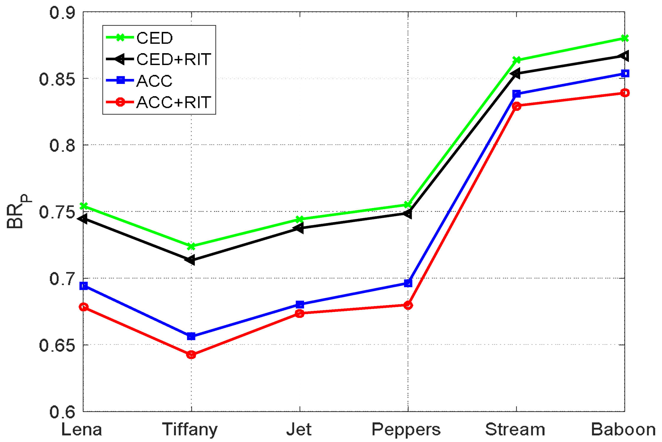
| Pure Bitrate | [16] | 1.77 | 1.75 | 1.76 | 1.79 | 1.88 | 1.87 |
| [17] | 1.86 | 1.82 | 1.86 | 1.86 | 1.95 | 1.94 | |
| [18] | 1.75 | 1.72 | 1.74 | 1.76 | 1.86 | 1.88 | |
| [19] | 1.82 | 1.78 | 1.80 | 1.83 | 1.94 | 1.92 | |
| Proposed | 1.68 | 1.64 | 1.67 | 1.68 | 1.83 | 1.84 |
© 2018 by the authors. Licensee MDPI, Basel, Switzerland. This article is an open access article distributed under the terms and conditions of the Creative Commons Attribution (CC BY) license (http://creativecommons.org/licenses/by/4.0/).
Share and Cite
Hong, W.; Zhou, X.; Weng, S. Joint Adaptive Coding and Reversible Data Hiding for AMBTC Compressed Images. Symmetry 2018, 10, 254. https://doi.org/10.3390/sym10070254
Hong W, Zhou X, Weng S. Joint Adaptive Coding and Reversible Data Hiding for AMBTC Compressed Images. Symmetry. 2018; 10(7):254. https://doi.org/10.3390/sym10070254
Chicago/Turabian StyleHong, Wien, Xiaoyu Zhou, and Shaowei Weng. 2018. "Joint Adaptive Coding and Reversible Data Hiding for AMBTC Compressed Images" Symmetry 10, no. 7: 254. https://doi.org/10.3390/sym10070254
APA StyleHong, W., Zhou, X., & Weng, S. (2018). Joint Adaptive Coding and Reversible Data Hiding for AMBTC Compressed Images. Symmetry, 10(7), 254. https://doi.org/10.3390/sym10070254