On the Convolution Quadrature Rule for Integral Transforms with Oscillatory Bessel Kernels

Abstract

Lubich’s convolution quadrature rule provides efficient approximations to integrals with special kernels. Particularly, when it is applied to computing highly oscillatory integrals, numerical tests show it does not suffer from fast oscillation. This paper is devoted to studying the convergence property of the convolution quadrature rule for highly oscillatory problems. With the help of operational calculus, the convergence rate of the convolution quadrature rule with respect to the frequency is derived. Furthermore, its application to highly oscillatory integral equations is also investigated. Numerical results are presented to verify the effectiveness of the convolution quadrature rule in solving highly oscillatory problems. It is found from theoretical and numerical results that the convolution quadrature rule for solving highly oscillatory problems is efficient and high-potential.

1. Introduction

Highly oscillatory integrals (HOI) arise frequently in antenna problems involving Sommerfeld integrals (see [1,2]), computation of mutual impedance between conductors (see [3,4]) and many other oscillatory problems (HOP). Generally, an oscillatory integral can be written as

$$\begin{array}{c}\hfill I\left[f\right]={\int }_0^{b}f(t)W(t)dt.\end{array}$$

(1)

Here $W(·)$ denotes a highly oscillatory function and $f(·)$ is slowly varied. Due to the high oscillation, classical quadrature rules (e.g., Newton-Cotes and Gauss rules ) are often ineffective, and calculation of this class of integrals is deemed to be a challenging problem ([5]).

Past decades witness a rapid development of researches on calculation of HOIs. Based on Filon’s idea ([6]), Iserles and Nørsett developed the Filon-type method by approximating the slowly varied function by its Hermite interpolant. Both of theoretical and numerical results manifested that this method enjoyed high-order convergence rates with respect to the frequency ([7]). To get stable and fast algorithms, Domínguez, et al. ([8]), and Xiang, et al. ([9]), proposed the Clenshaw-Curtis-Filon-type method, respectively, which enjoyed extensive applications at present.

Although Filon’s methodology leads to many efficient algorithms, most of them suffer to complicate computation of moment integrals. An alternative way to addressing this problem is transforming the integral interval into the complex plane, which derives the numerical steepest descent method. In [10], the complex integration method in the standard case was discussed extensively. In [11], the general form and corresponding error analysis were studied. This method was extended to the case of HOIs on semi-finite intervals in [12]. It is notable that the numerical steepest descent method with Gauss-Laguerre quadrature may not provide satisfactory solutions in practice (see [13]). Therefore, computation of transformed integrals is still an interesting topic.

Another important quadrature rule for HOIs is Levin’s method ([14]). It enjoys a wide application for its being free of computing complex moments and less restrictions to integrands. The spirit of this method is transforming the integration problem into an ODE, and solving this equation by collocation methods. It is well-know that implementing of Levin methods comes down to efficient solutions of linear systems, which are often singular and dense. In [15], an SVD solver for the ill-conditioned system was presented. In [16], Olver developed a moment-free method by using the shifted GMRES. Recently, by employing the property of Chebyshev polynomials and preconditioners, a sparse and well-conditioned Levin method was constructed in [17].

There are many other important methods for calculating HOIs, for example, the homotopy perturbation method ([18]), the generalized quadrature rule ([19]), the extrapolation method ([20]). For simplicity, we omit the details. It is quite unexpected that little attention has been paid to the convolution quadrature rule (CQ) for HOIs ([21,22]), especially its asymptotic property in the case of high oscillation. In fact, CQ is well-known for its efficient in evaluating convolution integrals, and oscillatory integrals of convolution-type play significant roles in solving oscillatory and evolutionary problems (see [23,24]). Therefore, it is a meaningful issue to study CQ for HOIs.

Consider integral transforms with Bessel kernels as

$$\begin{array}{c}\hfill {\int }_0^{x}f(t)J_m(\omega (x-t))dt,x\in [0,T],\end{array}$$

(2)

with $m\ge 0$ being an integer and $\omega \gg 1,$ and oscillatory Volterra integral equations as

$$\begin{array}{c}\hfill {\int }_0^x{J}_0(\omega (x-t))u(t)dt=f(x),x\in [0,T],\end{array}$$

(3)

where $f(·)$ is sufficiently smooth, $f(0)=0,$ and $u(t)$ is unknown. In this paper, we are devoted to studying convergence property of CQ with respective to the frequency for solving above two problems. The same models have been considered in [25,26], where authors concluded that Filon-type methods enjoyed the property that the higher the oscillation, the better the approximation. In the following, we will find CQ share a similar property as Filon-type methods, and even better when they are applied to solving highly oscillatory integral equations. The remaining parts are organized as follows. In Section 2, we briefly review CQ and give the convergence analysis. A modified rule is also proposed in this part. Then we study CQ for solving Volterra integral equations with highly oscillatory kernels in Section 3. Some numerical experiments are carried out in Section 4 to verify our given results.

2. Convergence of the Convolution Quadrature Rule

In this section, we revisit Lubich’s convolution quadrature firstly. Then the convergence property with respect to the frequency is studied. In [21,22], Lubich proposed an algorithm for computing the following integral,

$$\begin{array}{c}\hfill I[f,g]={\int }_0^{x}f(t)g(x-t)dt,x>0.\end{array}$$

(4)

Let $F(·)$ denote the Laplace transform of $f(·)$ and satisfy

• $F(s)$ is analytic in the region $|\arg (s-c)|<\pi -\phi ,\phi <\pi /2,c\in \mathbb{R};$
• there exist constants M and $\mu ,$ such that $|F(s)|\le {M|s|}^{-\mu }.$

By the definition of Laplace transform, it follows that

$$\begin{array}{c}\hfill f(t)=\frac{1}{2\pi i}{\int }_{\mathsf{\Gamma }}F(\lambda )e^{\lambda t}d\lambda ,\end{array}$$

(5)

where $\mathsf{\Gamma }$ is a curve locates in the analytic region of $F(s)$ and goes from ${\displaystyle \infty ·e^{-i(\pi -\phi )}}$ to ${\displaystyle \infty ·e^{i(\pi -\phi )}.}$

Substituting (5) into (4) gives

$$\begin{array}{c}\hfill {\int }_0^{x}f(t)g(x-t)dt=\frac{1}{2\pi i}{\int }_{\mathsf{\Gamma }}F(\lambda ){\int }_0^x{e}^{\lambda t}g(x-t)dtd\lambda .\end{array}$$

(6)

Noting that ${\displaystyle y(x)={\int }_0^x{e}^{\lambda t}g(x-t)dt}$ satisfies the initial value problem

$$\begin{array}{c}\hfill \left\{\begin{array}{c}{\displaystyle \frac{dy}{dx}=\lambda y(x)+g(x),}\hfill \\ {\displaystyle y(0)=0.}\hfill \end{array}\right.\end{array}$$

(7)

Defining the grid $\{t_n:=nh,n=0,1,\dots \},$ we can approximate $y(x)$ by

$$\begin{array}{c}\hfill \sum _{j=0}^k{\alpha }_j{y}_{n+j-k}=h\beta (\lambda y_n+g(nh)),n\ge 0,\end{array}$$

(8)

where $y_{-k}=\dots =y_{-1}=0,$ $g(x)=0(x<0).$ Multiplying both sides by ${\zeta }^n(n\ge 0)$ in (8) and summing give

$$\begin{array}{c}\hfill ({\alpha }_0{\zeta }^k+\dots +{\alpha }_k)\mathbf{y}(\zeta )=\beta (h\lambda \mathbf{y}(\zeta )+h\mathbf{g}(\zeta )),\end{array}$$

(9)

where ${\displaystyle \mathbf{y}(\zeta )=\sum _{n=0}^{\infty }{y}_n{\zeta }^n,\mathbf{g}(\zeta )=\sum _{n=0}^{\infty }g(nh){\zeta }^n.}$ Letting

$$\begin{array}{c}\hfill \delta (\zeta )=\frac{{\alpha }_0{\zeta }^k+\dots +{\alpha }_k}{\beta },\end{array}$$

(10)

it follows that

$$\begin{array}{c}\hfill \mathbf{y}(\zeta )={\left(\frac{\delta (\zeta )}{h}-\lambda \right)}^{-1}\mathbf{g}(\zeta ).\end{array}$$

(11)

Since $F(s)$ is analytic in the inside region of the curve $\mathsf{\Gamma },$ we have, by Cauchy’s integral formula (see [27], p. 32),

$$\begin{array}{c}\hfill \frac{1}{2\pi i}{\int }_{\mathsf{\Gamma }}F(\lambda ){\left(\frac{\delta (\zeta )}{h}-\lambda \right)}^{-1}d\lambda =F\left(\frac{\delta (\zeta )}{h}\right).\end{array}$$

(12)

Therefore, it follows that

$$\begin{array}{cc}\hfill \frac{1}{2\pi i}{\int }_{\mathsf{\Gamma }}F(\lambda )\mathbf{y}(\zeta )d\lambda =& \frac{1}{2\pi i}{\int }_{\mathsf{\Gamma }}F(\lambda ){\left(\frac{\delta (\zeta )}{h}-\lambda \right)}^{-1}\mathbf{g}(\zeta )d\lambda \hfill \\ \hfill =& F\left(\frac{\delta (\zeta )}{h}\right)\mathbf{g}(\zeta ).\hfill \end{array}$$

(13)

Here the coefficient corresponding to ${\zeta }^n$ denotes an approximation to the integral (4) at $x=nh.$ Suppose

$$\begin{array}{c}\hfill F\left(\frac{\delta (\zeta )}{h}\right)=\sum _{j=0}^{\infty }{w}_j(h){\zeta }^j.\end{array}$$

(14)

Then CQ for (4) is defined as

$$\begin{array}{c}\hfill Q_h^{cq}(x)=\sum _{0\le jh\le x}{w}_j(h)g(x-jh).\end{array}$$

(15)

By the definition of coefficients of Taylor expansions, we get

$$\begin{array}{c}\hfill w_n(h)=\frac{1}{2\pi i}{\int }_{|z|=\rho }F\left(\frac{\delta (\zeta )}{h}\right)z^{-n-1}dz,\end{array}$$

(16)

where $\rho$ is sufficiently small such that the disc $|z|\le \rho$ falls in the analytic region of ${\displaystyle F\left(\delta (\zeta )/h\right).}$ Letting ${\displaystyle z=\rho e^{i\theta },}$ we obtain

$$\begin{array}{c}\hfill w_n(h)=\frac{{\rho }^{-n}}{2\pi }{\int }_0^{2\pi }F\left(\frac{\delta (\rho e^{i\theta })}{h}\right)e^{-in\theta }d\theta .\end{array}$$

(17)

Discretizing ${\displaystyle {\int }_0^{2\pi }F\left(\frac{\delta (\rho e^{i\theta })}{h}\right)e^{-in\theta }d\theta }$ by the composite trapezoid rule gives

$$\begin{array}{cc}\hfill {\int }_0^{2\pi }F\left(\frac{\delta (\rho e^{i\theta })}{h}\right)e^{-in\theta }d\theta =& \sum _{l=0}^{L-1}{\int }_{l\frac{2\pi }{L}}^{(l+1)\frac{2\pi }{L}}F\left(\frac{\delta (\rho e^{i\theta })}{h}\right)e^{-in\theta }d\theta \hfill \\ \hfill \approx & \sum _{l=0}^{L-1}\frac{\pi }{L}\left(F\left(\frac{\delta (\rho e^{il\frac{2\pi }{L}})}{h}\right)e^{-inl\frac{2\pi }{L}}+F\left(\frac{\delta (\rho e^{i(l+1)\frac{2\pi }{L}})}{h}\right)e^{-in(l+1)\frac{2\pi }{L}}\right)\hfill \\ \hfill =& \frac{2\pi }{L}\sum _{l=0}^{L-1}F\left(\frac{\delta (\rho e^{il\frac{2\pi }{L}})}{h}\right)e^{-inl\frac{2\pi }{L}}.\hfill \end{array}$$

(18)

The last equal sign works due to ${\displaystyle F\left(\frac{\delta (\rho e^{i\theta })}{h}\right)e^{-in\theta }}$ is $2\pi -$periodic. This leads to

$$\begin{array}{c}\hfill w_n(h)\approx \frac{{\rho }^{-n}}{L}\sum _{l=0}^{L-1}F\left(\frac{\delta (\rho e^{il\frac{2\pi }{L}})}{h}\right)e^{-inl\frac{2\pi }{L}},n=0,1,\dots ,N.\end{array}$$

(19)

Its computation complexity is $O(NlogN)$ by FFT. In this paper, we adopt $L=10N,$ ${\rho }^N=\sqrt{ϵ},ϵ={10}^{-16}$ to guarantee a precision of order $O(\sqrt{ϵ})$ in (19).

Remark 1.

In [28], convolution quadrature weights were rewritten as

$$\begin{array}{c}\hfill w_j(h)={\int }_0^{\infty }g(s){\varphi }_j(s/h)ds.\end{array}$$

(20)

Here ${\displaystyle {\varphi }_j(t)=e^{-t}\frac{t^j}{j!}}$ for backward differentiation formula of order 1 (BDF1), and ${\displaystyle {\varphi }_j(t)=\frac{H_j(\sqrt{2t})}{j!}{\left(\frac{t}{2}\right)}^{j/2}{e}^{-3t/2}}$ for BDF2 with $H_j(·)$ denoting the jth Hermite polynomial. Recurrence relations of frequently-used bases can be found in

Table 1. Recurrence relations for the CQ basis functions.

Scheme	Initial Basis (${\mathit{\varphi }}_{-\mathit{n}}=0,\mathit{n}\ge 1$)	Recurrence for Basis Functions ($\mathit{j}\ge 1$)
BDF1	${\displaystyle {\varphi }_0(t)=e^{-t}}$	$j{\varphi }_j(t)-t{\varphi }_{j-1}(t)=0$
BDF2	${\displaystyle {\varphi }_0(t)=e^{-3t/2}}$	$j{\varphi }_j(t)-2t{\varphi }_{j-1}(t)+t{\varphi }_{j-2}(t)=0$
BDF3	${\displaystyle {\varphi }_0(t)=e^{-11t/6}}$	$j{\varphi }_j(t)-3t{\varphi }_{j-1}(t)+3t{\varphi }_{j-2}(t)-t{\varphi }_{j-3}(t)=0$
BDF4	${\displaystyle {\varphi }_0(t)=e^{-25t/12}}$	$j{\varphi }_j(t)-4t{\varphi }_{j-1}(t)+6t{\varphi }_{j-2}(t)-4t{\varphi }_{j-3}(t)+t{\varphi }_{j-4}(t)=0$

.

Existing convergence analysis of CQ often restricts to the property with respect to the stepsize. For example, setting

$$\begin{array}{cc}\hfill \mathcal{F}(s)g(x)=& {\int }_0^{x}f(t)g(x-t)dt,\hfill \end{array}$$

(21)

$$\begin{array}{cc}\hfill \mathcal{F}(s_h)g(x)=& \sum _{0\le jh\le x}{w}_j(h)g(x-jh),\hfill \end{array}$$

(22)

the convergence rate of CQ is as follows

Theorem 1.

([21], Theorem 3.1) Suppose that $\delta (\zeta )$ satisfies

• $\delta (\zeta )$ is analytic and without zeros in a neighbourhood of the closed unit disc $|\zeta |\le 1,$ with the exception of a zero at $\zeta =1;$
• $|arg\delta (\zeta )|\le \pi -\alpha ,$ for $|\zeta |<1,$ for some $\alpha >\phi ;$
• ${\displaystyle \frac{\delta (e^{-h})}{h}=1+O(h^p),}$ for some $p\ge 1.$

Then we have

$$\begin{array}{cc}\hfill |\mathcal{F}(s_h)g(x)-\mathcal{F}(s)g(x)|\le & C{x}^{\mu -1}\{h|g(0)|+\dots +h^{p-1}|g^{(p-2)}(0)|\hfill \\ & +h^p(|g^{(p-1)}(0)|+x\underset{0\le t\le x}{max}|g^{(p)}(t)|)\},\hfill \end{array}$$

(23)

where the constant C does not depend on the stepsize $h.$

One point which should be remarkable is that A-stable linear multistep methods for solving the initial value problem (7) are more reliable in actual computation. Therefore, in this paper, we make use of BDF2 in numerical experiments.

In the following parts, we study the convergence property of CQ for

$$\begin{array}{c}\hfill I\left[f\right]={\int }_0^{b}f(t)J_m(\omega t)dt,\omega \gg 1.\end{array}$$

(24)

Here $J_m(·)$ denotes the first kind Bessel function of order m with m being a nonnegative integer. Defining $\tilde{f}(s):=f(b-s),$ we transform (1) into

$$\begin{array}{c}\hfill I\left[f\right]={\int }_0^b\tilde{f}(b-s)J_m(\omega s)ds.\end{array}$$

(25)

Here the Laplace transform of $J_m(\omega s)$ can be represented as (see [29], p. 1024)

$$\begin{array}{c}\hfill F_{J_m}(s)=\frac{{\left(\sqrt{s^2+{\omega }^2}-s\right)}^m}{{\omega }^m\sqrt{s^2+{\omega }^2}}.\end{array}$$

(26)

Before elaborating on the convergence property of CQ, the following lemma should be presented first.

Lemma 1.

Suppose $f(·)$ is continuous on the interval $S,$ where S may be a closed interval on the positive real axis or $[a,\infty )$ for some $a\ge 0.$ Assume ${\displaystyle {\int }_S|f(t)|dt,}$ ${\displaystyle {\int }_S|f^{\prime }(t)|dt}$ exist. Then for any $v>0$ and sufficiently large $\omega ,$ there exists a constant $C,$ which does not depend on the frequency $\omega ,$ such that

$$\begin{array}{c}\hfill \left|{\int }_{S}f(t)J_m(\omega t)dt\right|\le C{\omega }^{-1}.\end{array}$$

(27)

Furthermore, if the interval S does not contain origin, then it follows

$$\begin{array}{c}\hfill \left|{\int }_{S}f(t)J_m(\omega t)dt\right|\le C{\omega }^{-3/2}.\end{array}$$

(28)

This lemma can be proved by integration by parts and we omit the detail. Now the main theorem of this section follows.

Theorem 2.

Suppose $f(·)\in C^2[0,b],$ and ${\displaystyle {\int }_0^b|f(t)|dt,}$ ${\displaystyle {\int }_0^b|f^{\prime }(t)|dt,}$ ${\displaystyle {\int }_0^b|f^{″}(t)|dt}$ exist. Then there exists a positive constant C independent of ω, such that, as the frequency ω tends to infinity, CQ satisfies

$$\begin{array}{c}\hfill |Q_h^{cq}(b)-I\left[f\right]|\le C{\omega }^{-3/2}.\end{array}$$

(29)

Proof. 

Denote by ${\delta }_j$ the coefficients of ${\displaystyle \delta (\zeta )=\sum _{j=0}^{\infty }{\delta }_j{\zeta }^j,}$ and define

$$\begin{array}{c}\hfill s_{h}g(x):=\frac{1}{h}\sum _{0\le jh\le x}{\delta }_{j}g(x-jh),0<x\le b.\end{array}$$

(30)

Then $I\left[f\right]$ can be represented as a Dunford-Taylor integral

$$\begin{array}{c}\hfill I\left[f\right]=\mathcal{F}(s_h)\tilde{f}(x)=\frac{1}{2\pi i}{\int }_{\mathsf{\Gamma }}{F}_{J_m}(\lambda ){(s_h-\lambda )}^{-1}\tilde{f}(x)d\lambda .\end{array}$$

(31)

By noting

$$\begin{array}{c}\hfill F_{J_m}(s)={\int }_0^{\infty }{e}^{-ts}{J}_m(\omega t)dt,\end{array}$$

(32)

we have

$$\begin{array}{cc}\hfill \mathcal{F}(s_h)\tilde{f}(x)=& \frac{1}{2\pi i}{\int }_{\mathsf{\Gamma }}{\int }_0^{\infty }{e}^{-t\lambda }{J}_m(\omega t){(s_h-\lambda )}^{-1}\tilde{f}(x)dtd\lambda \hfill \\ \hfill =& {\int }_0^{\infty }{J}_m(\omega t)e^{-t{s}_h}\tilde{f}(x)dt.\hfill \end{array}$$

(33)

This implies

$$\begin{array}{cc}\hfill \mathcal{F}(s_h)\tilde{f}(x)-\mathcal{F}(s)\tilde{f}(x)=& {\int }_0^x{J}_m(\omega t)(e^{-t{s}_h}\tilde{f}(x)-\tilde{f}(x-t))dt\hfill \\ & +{\int }_x^{\infty }{J}_m(\omega t)e^{-t{s}_h}\tilde{f}(x)dt.\hfill \end{array}$$

(34)

Define ${\displaystyle {\varphi }_1(t):=e^{-t{s}_h}\tilde{f}(x)-\tilde{f}\left(x-t\right)}$ and ${\displaystyle {\varphi }_2(t):=e^{-t{s}_h}\tilde{f}(x).}$ By recurrence relations and derivatives of Bessel functions, we get

$$\begin{array}{cc}\hfill \mathcal{F}(s_h)\tilde{f}(x)-\mathcal{F}(s)\tilde{f}(x)=& {\varphi }_1(0){\int }_0^x{J}_m(\omega t)dt+\frac{1}{\omega }({\varphi }_1(t)-{\varphi }_1(0))J_{m+1}(\omega t){|}_{t=0}^x\hfill \\ & -\frac{1}{\omega }{\int }_0^x\left({\varphi }_1^{\prime }(t)-\frac{m+1}{t}({\varphi }_1(t)-{\varphi }_1(0))\right)J_{m+1}(\omega t)dt\hfill \\ & +\frac{1}{\omega }{\varphi }_2(t)J_{m+1}(\omega t){|}_{t=x}^{\infty }\hfill \\ & -\frac{1}{\omega }{\int }_x^{\infty }\left({\varphi }_2^{\prime }(t)-\frac{m+1}{t}{\varphi }_2(t)\right)J_{m+1}(\omega t)dt.\hfill \end{array}$$

(35)

According to ${\varphi }_1(0)=0$ and Lemma 1, it follows

$$\begin{array}{c}\hfill |\mathcal{F}(s_h)\tilde{f}(x)-\mathcal{F}(s)\tilde{f}(x)|\le C{\omega }^{-3/2},\end{array}$$

(36)

where the constant C does not depend on $\omega .$ This completes the proof. ☐

This theorem verifies the accuracy of CQ will increase as the frequency tends to infinity. According to the proof of Theorem 2, we can eliminate low order terms in (35) and get a modified convolution quadrature rule.

• Modified convolution quadrature rule for (1) of the first kind (MCQ1).

  $$\begin{array}{cc}\hfill Q_h^{mcq1}(b)=& \mathcal{F}(s_h)(f(x)-f(b)){\mid }_{x=1}+f(b){\int }_0^b{J}_m(\omega t)dt.\hfill \end{array}$$

  (37)

According to ([30], p. 681), we have

$$\begin{array}{c}\hfill {\int }_0^1{t}^{\mu }{J}_{\nu }(\omega t)dt=\frac{2^{\mu }\mathsf{\Gamma }(\frac{\mu +\nu +1}{2})}{{\omega }^{\mu +1}\mathsf{\Gamma }(\frac{\nu -\mu +1}{2})}+{\omega }^{-\mu }(\mu +\nu -1)J_{\nu }(\omega )s_{\mu -1,\nu -1}^{(2)}(\omega )-{\omega }^{-\mu }{J}_{\nu -1}(\omega )s_{\mu ,\nu }^{(2)}(\omega ).\end{array}$$

(38)

Here $s_{\mu ,\nu }^{(2)}(x)$ denotes the Lommel function of the second kind, and can be efficient computed by asymptotic expansions ([31]). This implies

$$\begin{array}{c}\hfill {\int }_0^b{J}_m(\omega t)dt=\frac{1}{b^2\omega }+\frac{(m-1)J_m(\omega b)s_{-1,m-1}^{(2)}(\omega b)-J_{m-1}(\omega b)s_{0,m}^{(2)}(\omega b)}{b}.\end{array}$$

(39)

Analogy to the proof of Theorem 2, we immediately arrive at the following results.

Theorem 3.

Suppose $f(·)\in C^2[0,b],$ and ${\displaystyle {\int }_0^b|f(t)|dt,{\int }_0^b|f^{\prime }(t)|dt,{\int }_0^b|f^{″}(t)|dt}$ exist. Then there exists a positive constant C independent of ω, such that, as the frequency ω tends to infinity, MCQ1 satisfies

$$\begin{array}{c}\hfill |Q_h^{mcq1}(b)-I\left[f\right]|\le C{\omega }^{-2}.\end{array}$$

(40)

Remark 2.

By Lubich’s methodology of eliminating low order terms, we also obtain a modified convolution quadrature rule of the second kind for (1) (MCQ2). Although these two modified quadrature rules share the same convergence rates with respect to the stepsize, their convergence properties are quite different in the case of calculation of HOI. We will illustrate this phenomenon in Section 4.

3. Application to a Volterra Equation

In literature, convolution quadrature rules are important tools for solving Volterra equations with convolution kernels ([32]). Many numerical experiments show they are efficient for solving some highly oscillatory Volterra integral equations (HOVIE). Consider HOVIE (3),

$$\begin{array}{c}\hfill {\int }_0^x{J}_0(\omega (x-t))u(t)dt=f(x),x\in [0,T],\end{array}$$

where $f(·)$ is sufficiently smooth and $f(0)=0.$ Let

$$\begin{array}{c}\hfill I_N:=\{x_n:0=x_0<x_1<\dots <x_N=T\},\end{array}$$

(41)

be a uniform grid on $[0,T]$ with spacing $h:=T/N.$ This equation arises from acoustic scattering problems (see [33]). By applying CQ to (3), we get

$$\begin{array}{c}\hfill \sum _{j=0}^k{w}_{k-j}(h){\tilde{u}}_j=f_k,k=1,2,\dots ,N.\end{array}$$

(42)

Here $u_j$ denotes the numerical solution $\tilde{u}(x)$ at $x_j$ and $f_k:=f(x_k).$ Once the initial value $u_0$ is known, the numerical solution at the uniform grid $I_N$ can be obtained by solving the linear system (42), and the numerical solution on $[0,T]$ can be written as

$$\begin{array}{c}\hfill \tilde{u}(x):=\sum _{j=0}^N{\tilde{u}}_j{\varphi }_j(x).\end{array}$$

(43)

Following the methodology from [24,26], we establish the convergence analysis by expressing the error function in terms of moments with highly oscillatory kernels. So let us consider some integrals involving Bessel kernels.

Lemma 2.

Define the functional $T_x:C([0,T])\to R$ as

$$\begin{array}{c}\hfill T_x(f)={\int }_0^x{J}_m(\omega s)f(s)ds,\end{array}$$

(44)

with $x\in [0,T]$ and $f\in C([0,T]).$ Then $\infty -$norm of the functional $T_x$ satisfies

$$\begin{array}{c}\hfill \parallel T_x\parallel \le C{\omega }^{-1/2},\mathit{as}\omega \to \infty ,\end{array}$$

(45)

where C is a constant independent of $\omega .$

Proof. 

It is easy to show

$$\begin{array}{c}\hfill \parallel T_x\parallel ={\int }_0^x\mid J_m(\omega s)\mid ds.\end{array}$$

(46)

By the variable transformation $t=\omega s,$ we have

$$\begin{array}{c}\hfill \parallel T_x\parallel =\frac{1}{\omega }{\int }_0^{\omega x}\mid J_m(t)\mid dt.\end{array}$$

(47)

According to the asymptotic expansions of Bessel functions (see [34], p. 228), there exists $Z>0$ such that for any $z>Z,$ and a constant $C^{\ast },$ we have

$$\begin{array}{c}\hfill \mid J_m(z)\mid \le \frac{C^{\ast }}{\sqrt{z}}.\end{array}$$

(48)

This implies

$$\begin{array}{cc}\hfill \parallel T_x\parallel =& \frac{1}{\omega }{\int }_0^Z\mid J_m(t)\mid dt+\frac{1}{\omega }{\int }_Z^{\omega x}\mid J_m(t)\mid dt\hfill \\ \hfill \le & \frac{1}{\omega }{\int }_0^Z\mid J_m(t)\mid dt+\frac{1}{\omega }{\int }_Z^{\omega x}\frac{C^{\ast }}{\sqrt{z}}dt.\hfill \end{array}$$

(49)

Therefore, there exists a constant C, such that

$$\begin{array}{c}\hfill \parallel T_x\parallel \le C{\omega }^{-1/2},\mathrm{as}\omega \to \infty .\end{array}$$

(50)

This completes the proof. ☐

Lemma 3.

For any integers $\mu ,\nu >0$ and $x\in (0,T],$ the following integral

$$\begin{array}{c}\hfill I={\omega }^{1/2}{\int }_0^x\frac{J_{\mu }(\omega t)J_{\nu }(\omega (x-t))}{t}dt\end{array}$$

(51)

is uniformly bounded with respect to $\omega >0.$

Proof. 

The variable transformation $s=\omega t$ gives

$$\begin{array}{c}\hfill I={\omega }^{1/2}{\int }_0^{\omega x}\frac{J_{\mu }(s)J_{\nu }(\omega x-s)}{s}ds.\end{array}$$

(52)

According to ([34], p. 242), we have

$$\begin{array}{c}\hfill I=\frac{{\omega }^{1/2}{J}_{\mu +\nu }(\omega x)}{\mu }.\end{array}$$

(53)

By the asymptotic expansion of Bessel functions, we completes the proof. ☐

Now we get the convergence property of CQ for the numerical solution to HOVIE.

Theorem 4.

Suppose that $f\in C^3[0,T],$ then the convolution quadrature rule for solving (3) introduces a unique numerical solution $\tilde{u}$, and satisfies

$$\begin{array}{c}\hfill |u(x)-\tilde{u}(x)|\le C{\omega }^{-1/2},x\in I_N,\omega \to \infty ,\end{array}$$

(54)

where C is a constant independent of $\omega .$

Proof. 

By noting

$$\begin{array}{c}\hfill \mathcal{F}(s_h)\tilde{u}(x)=f(x)\end{array}$$

(55)

and

$$\begin{array}{c}\hfill \mathcal{F}(s)u(x)=f(x)\end{array}$$

(56)

with $x\in I_h,$ we get the error equation

$$\begin{array}{c}\hfill \mathcal{F}(s_h)ϵ(x)-(\mathcal{F}(s)u(x)-\mathcal{F}(s_h)u(x))=0,\end{array}$$

(57)

where $ϵ(x):=\tilde{u}(x)-u(x).$ By Remark 1 and Lemma 1, we have

$$\begin{array}{c}\hfill w_j(h)=\left\{\begin{array}{c}O({\omega }^{-1}),j=0,\hfill \\ O({\omega }^{-3/2}),j>0.\hfill \end{array}\right.\end{array}$$

(58)

Therefore, the remaining work is proving $\mathcal{F}(s)u(x)-\mathcal{F}(s_h)u(x)$ behaves as $O({\omega }^{-3/2}).$ A similar process to the proof of Theorem 2 gives

$$\begin{array}{cc}\hfill \mathcal{F}(s_h)u(x)-\mathcal{F}(s)u(x)=& {\varphi }_1(0){\int }_0^x{J}_0(\omega t)dt+\frac{1}{\omega }({\varphi }_1(t)-{\varphi }_1(0))J_1(\omega t){|}_0^x\hfill \\ & -\frac{1}{\omega }{\int }_0^x\left({\varphi }_1^{\prime }(t)-\frac{1}{t}({\varphi }_1(t)-{\varphi }_1(0))\right)J_1(\omega t)dt\hfill \\ & +\frac{1}{\omega }{\varphi }_2(t)J_1(\omega t){|}_x^{\infty }-\frac{1}{\omega }{\int }_x^{\infty }\left({\varphi }_2^{\prime }(t)-\frac{1}{t}{\varphi }_2(t)\right)J_1(\omega t)dt,\hfill \end{array}$$

(59)

where ${\varphi }_1(t):=e^{-t{s}_h}u(x)-u(x-t)$ and ${\varphi }_2(t):=e^{-t{s}_h}u(x).$ Consider the integrals

$$\begin{array}{c}\hfill \tilde{I}:={\int }_0^x\left({\varphi }_1^{\prime }(t)-\frac{1}{t}({\varphi }_1(t)-{\varphi }_1(0))\right)J_1(\omega t)dt+{\int }_x^{\infty }\left({\varphi }_2^{\prime }(t)-\frac{1}{t}{\varphi }_2(t)\right)J_1(\omega t)dt.\end{array}$$

(60)

By using integration by parts we have

$$\begin{array}{cc}\hfill \tilde{I}=& \frac{1}{\omega }\left({\varphi }_1^{\prime }(t)-\frac{{\varphi }_1(t)}{t}\right)J_2(\omega t){|}_0^x-\frac{1}{\omega }{\int }_0^x\frac{t^2{\varphi }_1^{″}(t)-3t{\varphi }_1^{\prime }(t)+3{\varphi }_1(t)}{t^2}{J}_2(\omega t)dt\hfill \\ & +\frac{1}{\omega }\left({\varphi }_2^{\prime }(t)-\frac{{\varphi }_2(t)}{t}\right)J_2(\omega t){|}_x^{\infty }-\frac{1}{\omega }{\int }_x^{\infty }\left({\varphi }_2^{″}(t)-\frac{3{\varphi }_2^{\prime }(t)}{t}+\frac{3{\varphi }_2(t)}{t^2}\right)J_2(\omega t)dt.\hfill \end{array}$$

(61)

According to [35], the exact solution to (3) can be written as

$$\begin{array}{c}\hfill u(x)=f^{\prime }(x)+{\omega }^2{\int }_0^x{J}_0(\omega s)f(x-s)ds-\omega {\int }_0^x{J}_1(\omega s)f^{\prime }(x-s)ds.\end{array}$$

(62)

Furthermore, we have

$$\begin{array}{cc}\hfill u^{\prime }(x)=& f^{″}(x)+{\omega }^2{\int }_0^x{J}_0(\omega s)f^{\prime }(x-s)ds-\omega J_1(\omega x)f^{\prime }(0)-\omega {\int }_0^x{J}_1(\omega s)f^{″}(x-s)ds,\hfill \end{array}$$

(63)

$$\begin{array}{cc}\hfill u^{″}(x)=& f^{‴}(x)+\frac{\omega J_1(\omega x)}{x}{f}^{\prime }(0)+\omega {\int }_0^x\frac{J_1(\omega s)}{s}{f}^{″}(x-s)ds.\hfill \end{array}$$

(64)

A direct calculation implies ${\displaystyle \frac{t^2{\varphi }_1^{″}(t)-3t{\varphi }_1^{\prime }(t)+3{\varphi }_1(t)}{t^2}+\frac{\omega J_1(\omega (x-t))}{x-t}{f}^{\prime }(0)}$ is $O(\omega )$ as $\omega$ goes to infinity. By Lemmas 2 and 3, we obtain

$$\begin{array}{c}\hfill \left|{\int }_0^x\frac{t^2{\varphi }_1^{″}(t)-3t{\varphi }_1^{\prime }(t)+3{\varphi }_1(t)}{t^2}{J}_2(\omega t)dt\right|\sim O({\omega }^{1/2}),\omega \to \infty .\end{array}$$

(65)

With the help of Lemma 1, we have $\tilde{I}=O({\omega }^{-1/2}).$ It follows that

$$\begin{array}{c}\hfill \mid \mathcal{F}(s)u(x)-\mathcal{F}(s_h)u(x)\mid =O({\omega }^{-3/2}).\end{array}$$

(66)

Combining Equations (58) and (66) gives

$$\begin{array}{c}\hfill |u(x)-\tilde{u}(x)|\le C{\omega }^{-1/2},x\in I,\omega \to \infty ,\end{array}$$

(67)

where C is a constant independent of $\omega .$ This completes the proof. ☐

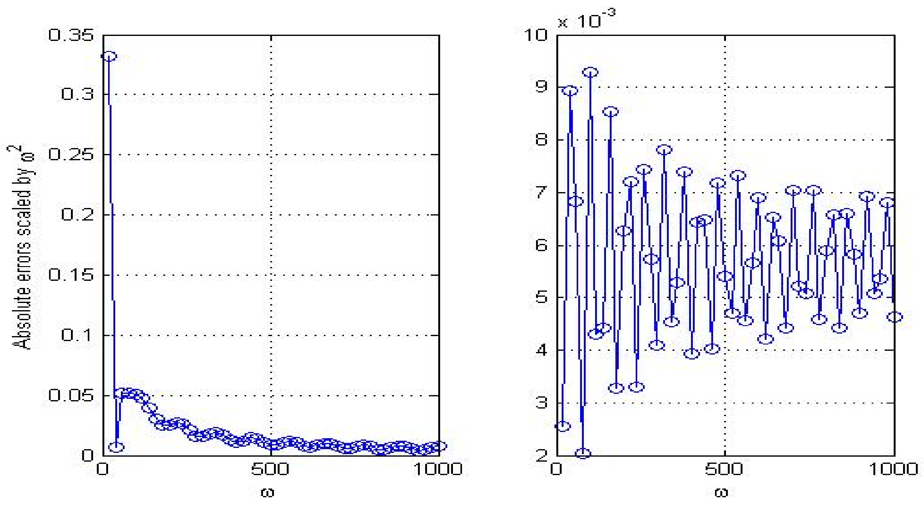
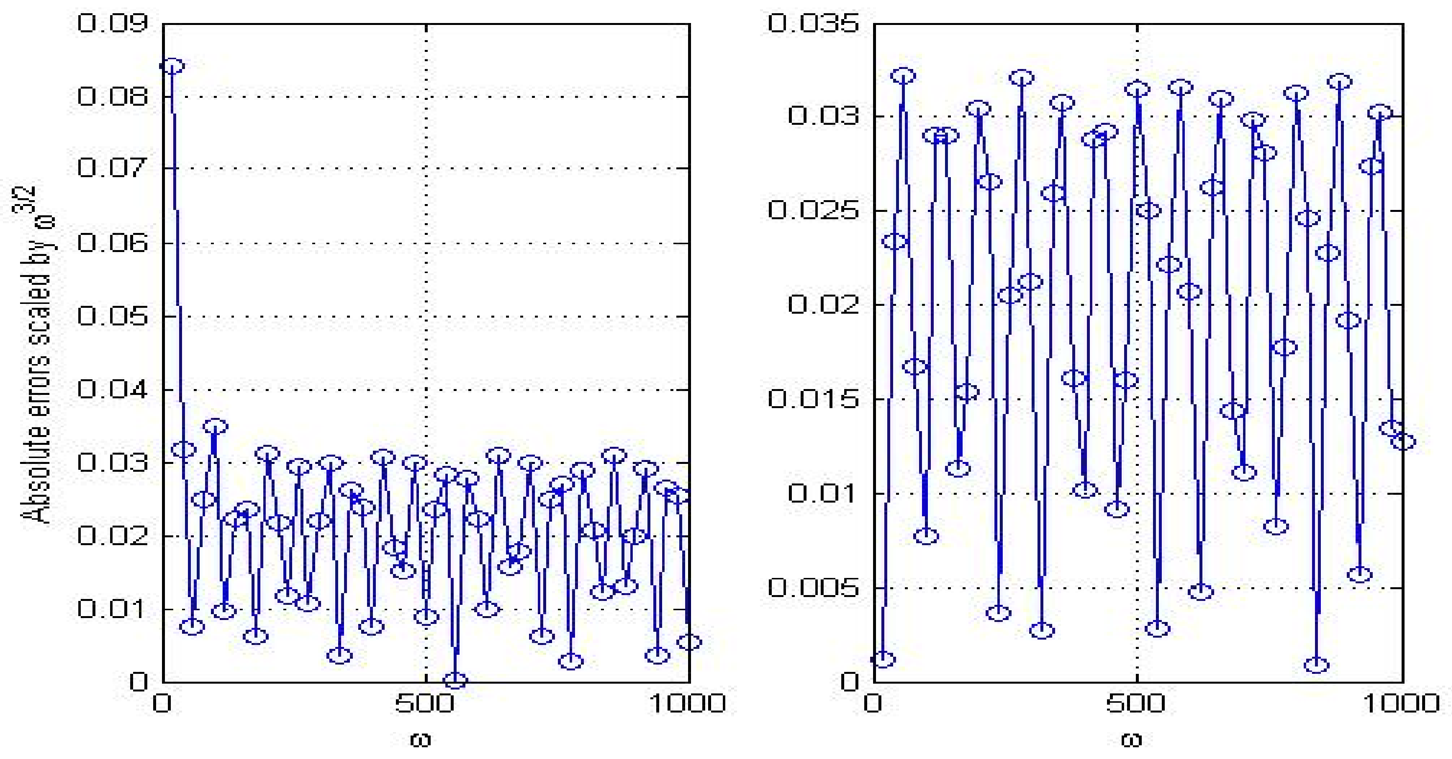
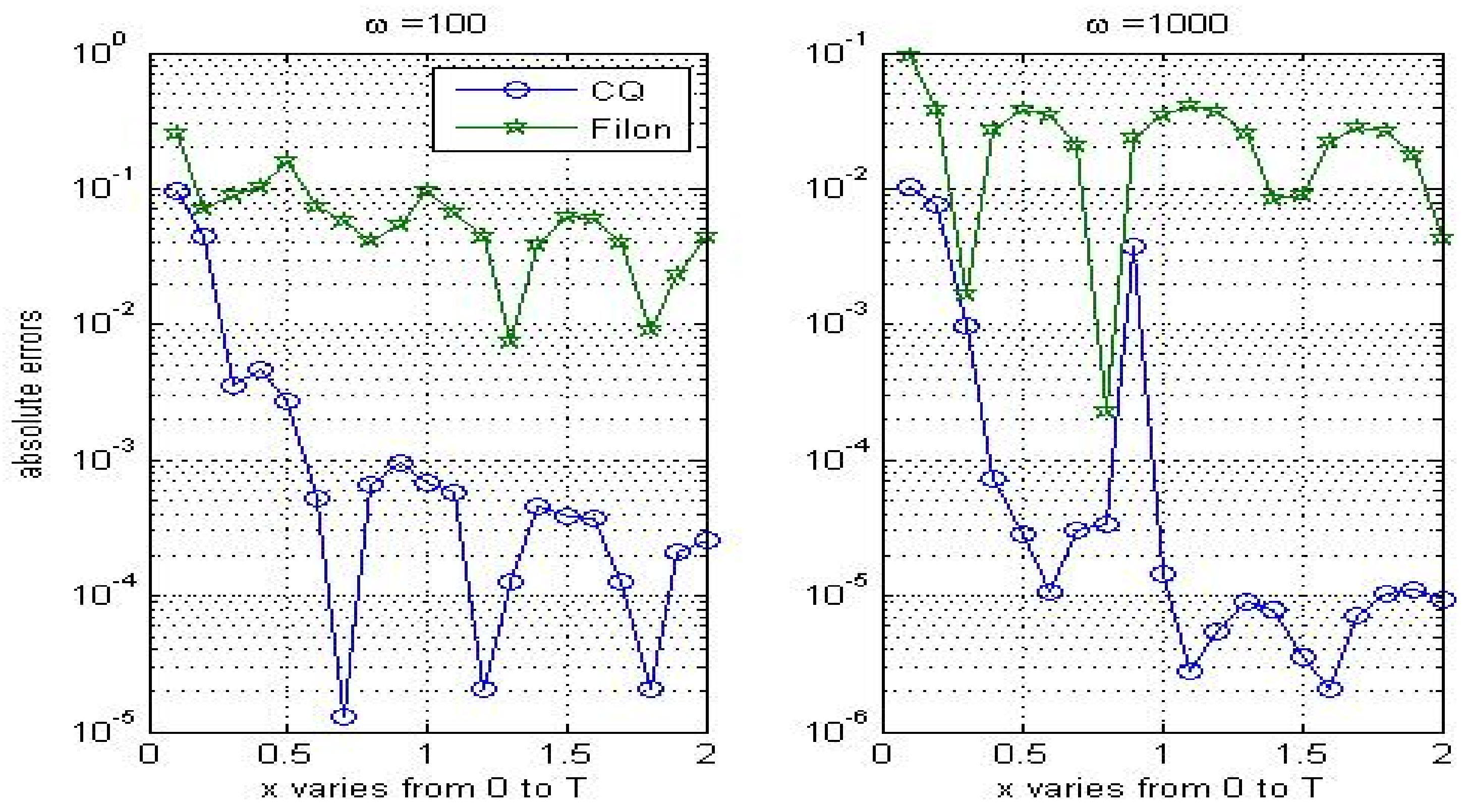
4. Numerical Results

In this section, we present some numerical results to verify given estimates in previous sections. All experiments are performed in Matlab 2013b.

As a first example, we consider the following HOI,

$$\begin{array}{c}\hfill I_1={\int }_0^1{J}_0(\omega t)\frac{1}{1+25t^2}dt,I_2={\int }_0^2{J}_1(\omega t)cos(t){\mathrm{e}}^{-t}dt.\end{array}$$

(68)

In Figure 1, Figure 2 and Figure 3, we show the convergence rates of three convolution quadrature rules. Slowly varied lines in these figures manifest that given asymptotic orders in Section 2 are optimal. Absolute errors of these methods are given in

Table 2. Comparisons of quadrature rules for ${\displaystyle {\int }_0^1{J}_0(\omega t)\frac{1}{1+25t^2}dt.}$

$\mathit{\omega }$	20	100	200	400	600	800	1000
CQ	$9.7\times {10}^{-4}$	$3.4\times {10}^{-5}$	$1.1\times {10}^{-5}$	$9.4\times {10}^{-7}$	$1.5\times {10}^{-6}$	$1.3\times {10}^{-6}$	$1.7\times {10}^{-7}$
MCQ1	$8.3\times {10}^{-4}$	$5.0\times {10}^{-6}$	$6.3\times {10}^{-7}$	$6.6\times {10}^{-8}$	$2.1\times {10}^{-8}$	$1.2\times {10}^{-8}$	$7.2\times {10}^{-9}$
MCQ2	$9.4\times {10}^{-4}$	$3.5\times {10}^{-5}$	$1.1\times {10}^{-5}$	$9.4\times {10}^{-7}$	$1.5\times {10}^{-6}$	$1.3\times {10}^{-6}$	$1.7\times {10}^{-7}$

and

Table 3. Comparisons of quadrature rules for ${\displaystyle {\int }_0^2{J}_1(\omega t)cos(t){\mathrm{e}}^{-t}dt.}$

$\mathit{\omega }$	20	100	200	400	600	800	1000
CQ	$1.3\times {10}^{-5}$	$7.8\times {10}^{-6}$	$1.1\times {10}^{-5}$	$1.3\times {10}^{-6}$	$1.4\times {10}^{-6}$	$1.4\times {10}^{-6}$	$4.0\times {10}^{-7}$
MCQ1	$6.3\times {10}^{-6}$	$9.3\times {10}^{-7}$	$1.6\times {10}^{-7}$	$2.5\times {10}^{-8}$	$1.9\times {10}^{-8}$	$9.2\times {10}^{-9}$	$4.6\times {10}^{-9}$
MCQ2	$1.3\times {10}^{-5}$	$7.8\times {10}^{-6}$	$1.1\times {10}^{-5}$	$1.3\times {10}^{-6}$	$1.4\times {10}^{-6}$	$1.4\times {10}^{-6}$	$4.0\times {10}^{-7}$

. The numerical results illustrate MCQ1 is much more efficient than other two methods in computing HOI.

In the second example, we consider application of CQ to solving HOVIE (3). Firstly, by letting $T=2$ and $N=20,$ we give the computed solution in

Table 4. CQ for Volterra integral equations with ${\displaystyle f(x)=x{\mathrm{e}}^{-x}.}$

$\mathit{\omega }$	$\mathit{x}=0.1$	$\mathit{x}=0.4$	$\mathit{x}=0.8$	$\mathit{x}=1.2$	$\mathit{x}=1.6$	$\mathit{x}=1.8$	$\mathit{x}=2$
10	$3.3\times {10}^{-1}$	$7.6\times {10}^{-2}$	$4.7\times {10}^{-2}$	$2.5\times {10}^{-2}$	$8.0\times {10}^{-3}$	$1.4\times {10}^{-2}$	$3.1\times {10}^{-3}$
100	$9.1\times {10}^{-2}$	$5.5\times {10}^{-3}$	$6.3\times {10}^{-4}$	$7.0\times {10}^{-5}$	$3.5\times {10}^{-4}$	$3.6\times {10}^{-5}$	$2.6\times {10}^{-4}$
200	$5.0\times {10}^{-2}$	$1.4\times {10}^{-4}$	$3.6\times {10}^{-4}$	$1.1\times {10}^{-4}$	$1.2\times {10}^{-4}$	$1.1\times {10}^{-4}$	$1.8\times {10}^{-5}$
500	$1.9\times {10}^{-2}$	$1.9\times {10}^{-4}$	$1.2\times {10}^{-5}$	$4.6\times {10}^{-5}$	$3.7\times {10}^{-5}$	$2.2\times {10}^{-5}$	$6.8\times {10}^{-6}$
1000	$1.0\times {10}^{-2}$	$5.9\times {10}^{-7}$	$3.9\times {10}^{-5}$	$1.2\times {10}^{-5}$	$8.7\times {10}^{-10}$	$9.6\times {10}^{-6}$	$9.2\times {10}^{-6}$

with various $\omega .$ Absolute errors listed in this table show CQ shares the same property as Filon methods ([24,26]), that is, the higher the oscillation, the better the approximation. Then we compare these two methods in Figure 4, where we can learn CQ behaves better than Filon methods.

5. Conclusions

The above theoretical and numerical results contribute to the study on the convergence property of CQ for solving HOP. The theoretical results in Section 2 reveal the convergence rate of CQ with respect to the frequency, that is, CQ converges in negative powers of $\omega$ as $\omega$ goes to infinity. Among them, the new modified rule (MCQ1) enjoys the fastest convergence rate. When we apply CQ to solving HOVIE, similar phenomenon is detected and analyzed. The numerical results in Section 4 show given convergence orders in Section 2 are optimal. In addition, this paper merely opens a window to the convergence theory of CQ for HOP, much work on various versions of CQ, such as Runge-Kutta CQ ([36]), Fourier CQ ([37]), and so forth, is needed in the future.

References

1. Michalski, K. Extrapolation methods for sommerfeld integral tails. IEEE Trans. Antennas Propag. 1998, 46, 1405–1418. [Google Scholar] [CrossRef]
2. Rakov, V.; Uman, M. Review and evaluation of lightning return stroke models including some aspects of their application. IEEE Trans. Electromagn. C 1998, 40, 403–426. [Google Scholar] [CrossRef]
3. Theodoulidis, T. Exact solution of Pollaczek’s integral for evaluation of earth-return impedane for underground conductors. IEEE Trans. Electromagn. C 2012, 54, 806–814. [Google Scholar] [CrossRef]
4. Ma, J. Fast and high-precision calculation of earth return mutual impedance between conductors over a multilayered soil. COMPEL 2018, 37, 1214–1227. [Google Scholar] [CrossRef]
5. Iserles, A. On the numerical quadrature of highly-oscillating integrals I: Fourier transforms. IMA J. Numer. Anal. 2004, 24, 365–391. [Google Scholar] [CrossRef] [Green Version]
6. Filon, L.N.G. On a quadrature formula for trigonometric integrals. Proc. R. Soc. Edinb. 1928, 49, 38–47. [Google Scholar] [CrossRef]
7. Iserles, A.; Nørsett, S.P. Efficient quadrature of highly oscillatory integrals using derivatives. Proc. R. Soc. A 2005, 461, 1383–1399. [Google Scholar] [CrossRef] [Green Version]
8. Domínguez, V.; Graham, I.G.; Smyshlyaev, V.P. Stability and error estimates for Filon-Clenshaw-Curtis rules for highly-oscillatory integrals. IMA J. Numer. Anal. 2011, 31, 1253–1280. [Google Scholar] [CrossRef]
9. Xiang, S.; Cho, Y.; Wang, H.; Brunner, H. Clenshaw-Curtis-Filon-type methods for highly oscillatory Bessel transforms and applications. IMA J. Numer. Anal. 2011, 31, 1281–1314. [Google Scholar] [CrossRef]
10. Milovanovíc, G. Numerical calculation of integrals involving oscillatory and singular kernels and some applications of quadratures. Comput. Math. Appl. 1998, 36, 19–39. [Google Scholar] [CrossRef]
11. Huybrechs, D.; Vandewalle, S. On the evaluation of highly oscillatory integrals by analytic continuation. SIAM J. Numer. Anal. 2006, 44, 1026–1048. [Google Scholar] [CrossRef]
12. Majidian, H. Numerical approximation of highly oscillatory integrals on semi-finite intervals by steepest descent method. Numer. Algorithms 2013, 63, 537–548. [Google Scholar] [CrossRef]
13. Ma, J. Implementing the complex integral method with the transformed Clenshaw-Curtis quadrature. Appl. Math. Comput. 2015, 250, 792–797. [Google Scholar] [CrossRef]
14. Levin, D. Procedures for computing one- and two-dimensional integrals of functions with rapid irregular oscillations. Math. Comput. 1982, 38, 531–538. [Google Scholar] [CrossRef]
15. Li, J.; Wang, X.; Wang, T. A universal solution to one-dimensional highly oscillatory integrals. Sci. China 2008, 10, 1614–1622. [Google Scholar]
16. Olver, S. Shifted GMRES for oscillatory integrals. Numer. Math. 2010, 114, 607–628. [Google Scholar] [CrossRef]
17. Ma, J.; Liu, H. A well-conditioned Levin method for calculation of highly oscillatory integrals and its application. J. Comput. Appl. Math. 2018, 342, 451–462. [Google Scholar] [CrossRef]
18. Chen, R.; Xiang, S. Note on the homotopy perturbation method for multivariate vector-value oscillatory integrals. Appl. Math. Comput. 2009, 215, 78–84. [Google Scholar] [CrossRef]
19. Evans, G.A.; Chung, K.C. Some theoretical aspects of generalised quadrature rules. J. Complex. 2003, 19, 272–285. [Google Scholar] [CrossRef]
20. Sidi, A. Extrapolation method for oscillatory infinite integrals. Math. Comput. 1988, 51, 249–266. [Google Scholar] [CrossRef]
21. Lubich, C. Convolution quadrature and discretized operational calculus. I. Numer. Math. 1988, 52, 129–145. [Google Scholar] [CrossRef]
22. Lubich, C. Convolution quadrature and discretized operational calculus. II. Numer. Math. 1988, 52, 413–425. [Google Scholar] [CrossRef]
23. Lubich, C. On convolution quadrature and Hille-Phillips operational calculus. Appl. Numer. Math. 1992, 9, 187–199. [Google Scholar] [CrossRef]
24. Xiang, S.; Brunner, H. Efficient methods for Volterra integral equations with highly oscillatory Bessel kernels. BIT Numer. Math. 2013, 53, 241–263. [Google Scholar] [CrossRef]
25. Xiang, S.; Wang, H. Fast integration of highly oscillatory integrals with exotic oscillators. Math. Comput. 2010, 79, 829–844. [Google Scholar] [CrossRef]
26. Ma, J.; Xiang, S.; Kang, H. On the convergence rates of Filon methods for the solution of a Volterra integral equation with a highly oscillatory Bessel kernel. Appl. Math. Lett. 2013, 26, 699–705. [Google Scholar] [CrossRef]
27. Stein, M.S.; Shakarchi, R. Complex Analysis; Princeton University Press: Princeton, NJ, USA, 2003. [Google Scholar]
28. Davis, P.; Duncan, D. Convolution spline approximations for time domain boundary integral equations. J. Integral Equ. Appl. 2014, 26, 369–410. [Google Scholar] [CrossRef] [Green Version]
29. Abramowitz, M.; Stegun, I.A. Handbook of Mathematical Functions; Dover Publications: Mineola, NY, USA, 1964. [Google Scholar]
30. Gradshteyn, I.S.; Ryzhik, I.M. Table of Integrals, Series, and Products; Academic Press: Cambridge, MA, USA, 1994. [Google Scholar]
31. Watson, G.N. A Treatise on the Theory of Bessel Functions; Cambridge University Press: Cambridge, UK, 1952. [Google Scholar]
32. Kauthen, J.P. A survey of singularly perturbed Volterra equations. Appl. Numer. Math. 1997, 24, 95–114. [Google Scholar] [CrossRef]
33. Davis, P.; Duncan, D. Stability and convergence of collocation schemes for retarded potential integral equations. SIAM J. Numer. Anal. 2004, 42, 1167–1188. [Google Scholar] [CrossRef]
34. Olver, F.J.; Lozier, D.W.; Boisvert, R.F.; Clark, C.W. NIST Handbook of Mathematical Functions; Cambridge University Press: Cambridge, UK, 2010. [Google Scholar]
35. Wang, H.; Xiang, S. Asymptotic expansion and Filon-type methods for a Volterra integral equation with a highly oscillatory kernel. IMA J. Numer. Anal. 2011, 31, 469–490. [Google Scholar] [CrossRef]
36. Banjai, L.; Lubich, C.; Melenk, J.M. Runge-Kutta convolution quadrature for operators arising in wave propagation. Numer. Math. 2011, 119, 1–20. [Google Scholar] [CrossRef]
37. Xu, K.; Austin, A.P.; Wei, K. A Fast Algorithm for the Convolution of Functions with Compact Support Using Fourier Extensions. SIAM J. Sci. Comput. 2017, 39, A3089–A3106. [Google Scholar] [CrossRef]
Figure 1. Asymptotic convergence rates of CQ for 0 1 J 0 ( ω t ) 1 1 + 25 t 2 d t (left) and 0 2 J 1 ( ω t ) cos ( t ) e t d t (right).
Symmetry 10 00239 g001
Figure 2. Asymptotic convergence rates of MCQ1 for 0 1 J 0 ( ω t ) 1 1 + 25 t 2 d t (left) and 0 2 J 1 ( ω t ) cos ( t ) e t d t (right).
Symmetry 10 00239 g002
Figure 3. Asymptotic convergence rates of MCQ2 for 0 1 J 0 ( ω t ) 1 1 + 25 t 2 d t (left) and 0 2 J 1 ( ω t ) cos ( t ) e t d t (right).
Symmetry 10 00239 g003
Figure 4. Comparisons between Filon methods and CQ for solving Volterra equations with f ( x ) = x 1 + x 2 .
Symmetry 10 00239 g004