Towards Real-Time Facial Landmark Detection in Depth Data Using Auxiliary Information

Abstract

Modern facial motion capture systems employ a two-pronged approach for capturing and rendering facial motion. Visual data (2D) is used for tracking the facial features and predicting facial expression, whereas Depth (3D) data is used to build a series of expressions on 3D face models. An issue with modern research approaches is the use of a single data stream that provides little indication of the 3D facial structure. We compare and analyse the performance of Convolutional Neural Networks (CNN) using visual, Depth and merged data to identify facial features in real-time using a Depth sensor. First, we review the facial landmarking algorithms and its datasets for Depth data. We address the limitation of the current datasets by introducing the Kinect One Expression Dataset (KOED). Then, we propose the use of CNNs for the single data stream and merged data streams for facial landmark detection. We contribute to existing work by performing a full evaluation on which streams are the most effective for the field of facial landmarking. Furthermore, we improve upon the existing work by extending neural networks to predict into 3D landmarks in real-time with additional observations on the impact of using 2D landmarks as auxiliary information. We evaluate the performance by using Mean Square Error (MSE) and Mean Average Error (MAE). We observe that the single data stream predicts accurate facial landmarks on Depth data when auxiliary information is used to train the network. The codes and dataset used in this paper will be made available.

1. Introduction

Motion capture using visual cameras is a common practice in high-end facial animation production. Commercial companies have a preference towards optical marker based systems, such as Vicon [1] as they allow for a large quantity of tracked landmarks with high accuracy. Additionally, with optical markers the addition of multiple cameras allows Depth information to be predicted. However, the set up time of the tracking markers is lengthy and prone to human error. A solution to this is to implement marker-less tracking, which uses visual cameras, computer vision techniques and machine learning to label facial features [2,3]. Marker-less tracking, currently, cannot track as accurately or as many points as optical marker systems. Similarly, to optical markers, additional cameras allow capture of Depth information. However, with technology advancements, the prices of Depth sensors have decreased, while they have significant performance improvements, making them suitable for consumer based production. Additionally, with the availability of RGB with Depth (RGBD) sensors, the potential to increase accuracy is possible by merging the data streams within a neural network. Merging RGB and Depth allows a marker-less system to predict Depth without the requirement of multiple cameras with high accuracy. The Depth information assists greatly in identifying facial feature movement and synthesising to 3D models. Furthermore, in object recognition Greyscale (Gs) outperforms RGB data significantly [4]. Thus we also compare against Gs image and merged Greyscale with Depth (GsD). This study improves upon current work, as the literature is split between networks that use full RGB [2,3] and networks that run Gs [5,6] without justification, and focuses solely on 2D landmarks prediction. 3D landmarks are important for face recognition in the presence of expressions [7] and real-time facial animation [8]. To do this, we extend the existing work to predict 3D landmarks and investigate the impact on 2D and 3D data if they are used as auxiliary information.

As with many fields of research, the implementation of deep learning has shown significant improvements in facial landmarking [9], when compared to traditional machine learning [10]. In this work, we focus on the use of CNNs, like the literature in this area. To perform the experimentation, we develop near identical networks to reduce the deviation between results. Our main contributions are:

• We introduce a new Kinect One [11] dataset, namely KOED to overcome data deficiency in this domain.
• We propose a novel and automated real-time 3D facial landmarks detection method.
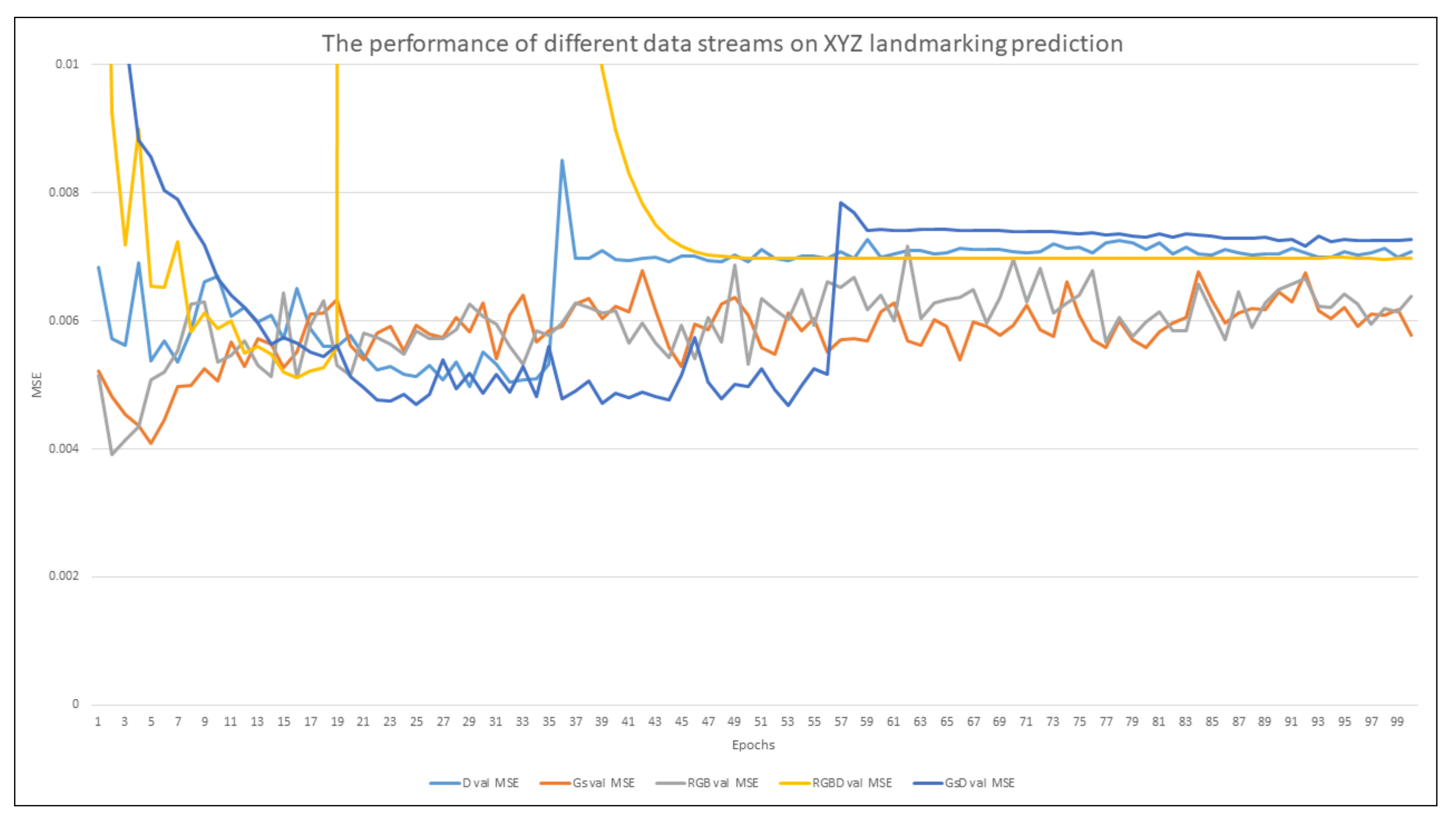
• We conduct a complete investigation on the effect of different data streams, such as Gs, RGB, GsD, RGBD in 2D and 3D facial landmarks detection.

By performing this investigation, we can determine the best solution for automated real-time 3D landmarks detection.

2. Related Work

The related work is divided into three sections. Firstly, we give an overview of the current state-of-the-art deep learning to predict facial landmarks. We demonstrate the key aspects of the networks functionality and the features used to localise landmark regions. The second section evaluates merging Gs/RGB and Depth information in a neural network and the current implementation methods. Lastly, we present a review of existing 3D datasets and their limitations.

2.1. Facial Landmarking with Neural Networks

Facial landmarking in deep learning is well established, with state of the art showing both real-time and high accuracy results. Neural networks have solved a wide range of problems, such as facial landmarking, age identification and gender classification. Due to the adaptability of neural networks, previous literature has evolved to use multi-output networks [12,13]. Multi-output networks perform an array of predictions simultaneously, such as age and gender. For our review, we focus on both single and multi-output networks, such as landmark and gender [3] and landmarking only networks. We discuss multiple output networks as they can outperform landmarking only networks as research shows that auxiliary features have a positive effect on network performance [14]. Auxiliary features boost network performance by adding key pieces of information. For example, in age prediction, if gender is used as an auxiliary feature, it aids the network as it learns how the make-up and facial hair affect age prediction. Auxiliary information is predicted by the network in addition to other outputs; the input to the networks is still a single or merged stream of data. Our experiment seeks to observe the effect of different streams of data on a neural network; the area of facial landmarking using auxiliary features, such as age and gender, would be an aspect of future work.

We first evaluate networks that focus solely on the prediction of landmarks. In 2013, Sun et al. [15] proposed an end-to-end network that takes a facial image through a series of convolutions, max-pooling, and fully connected layers, to predict five facial landmarks with reasonable accuracy. Zhou et al. [5] expanded on the work, by proposing a series of detectors to identify facial regions and process them by small neural networks. They also use a refinement approach that aligns the facial features before landmark prediction. Lia et al. [16] proposed a complex network for landmark detection where they implemented a two-stage network, the first stage is a series of convolution and deconvolution layers to process the image given into a high-value feature set. The features were then processed by a series of LSTM [17] layers to identify and refine the landmark position. Recently, Liu et al. [18] used a multitude of facial feature detectors to identify regions, such as eyes, nose, and mouth. The authors processed these regions with small sized neural networks that identify the landmarks on each of the features. This method achieves high accuracy results, as the network and detectors specialise in different aspects of the face, instead of trying to generalise to all the unique features. However, unlike Zhou et al. [5], they did not align the features.

We now review the work that uses multiple output networks. Zhang et al. [12] experimented in the use of auxiliary features to increase a network understanding of facial structure and features. They created multiple networks with the structure remaining the same except for the outputs changing by adding key pieces of information such as facial direction, age, and gender. By incorporating auxiliary features, networks learned facial features in more Depth. The authors observed a significant increase in accuracy when asking the network to determine these extra features, even when training the network to perform normally difficult tasks, such as facial direction. More recently, Zhang et al. [14] extended their work on facial alignment. Jourabloo et al. [6] used a similar method to predict landmarks by having a series of networks refine the positions. However, they focused on using the landmarks to refine the appearance of a 3D model. Even though Zhang et al. [14] and Jourabloo et al. [6] provide high accuracy networks, the networks require pre-processing to crop faces out of the image.

Finally, we review all-in-one networks, where no pre-processing is required before network prediction. The most recent research for facial landmarking focused on end-to-end networks based upon Recurrent Neural Networks (RNN) [19]. Zhang et al. [2] presented an all-in-one neural network to identify and landmark faces in an image. They used three interlinked networks to refine the landmarking approach. The result of the network is five facial landmarks and bounding box for every face in an image. On the other hand, Ranjan et al. [3] produced their all-in-one network to retrieve the face bounding box, landmark, facial direction and gender with high accuracy. The network included a separate classifier to check if the first section of the network returned a true face.

The networks, when trained on the separate streams of data, give high-end accuracy results starting from the small-scale one output networks to complex multi-model methods. However, the work is limited as it only considers single RGB or Gs images to predict 2D landmarks. Whereas state of art uses multiple cameras or Depth data to estimate the desired 3D landmarks. Additionally, the literature does not give justification for the use of either RGB or Gs. As neural networks are adaptable, we want to investigate how the different streams of data affect a neural network’s ability to predict both 2D and 3D landmarks. Furthermore, we extend this by analysing the effect of merging multiple data streams for accurate facial landmark prediction, such as integrating both RGB or Gs with Depth. We also extend on Zhou et al.’s [5] work by analysing the effect of using UV and XYZ as auxiliary features, compared to using UV or XYZ only to train a model that understands facial structure in detail.

Investigation of the use of Depth information to predict facial landmarking has been performed [20]. However, much of the focus is on using surface curvature analysis. Curvature analysis does give reasonable results on low noise models, but it is a slow process and can only track a few points in areas of high curvature change. Another method of predicting 3D facial landmarks is shown by Nair et al. [21], who impressively have predicted a total of 49 landmarks on the face, but they avoid the mouth area. However, this method required a generated 3D model, as point distributed model is used to deform a template face with landmarks assigned to the new mesh. This is an intense and computationally expensive task. Both methods required pre-generated models that are difficult at real-time on a consumer base; our focus is the sole use of images to accurately infer the landmarks.

2.2. Merging Visual and Depth

A multi-model network [22] for the merging of data, such as Gs and Depth, usually implements three separate networks that work together. The first two networks take input from the separate streams of data; then they can be processed the same way as a traditional CNNs. The network uses these convolutions to extract the unique features in each of the data streams. After the processing, the inputs for unique features the outputs are fed into the third neural network and the data merged using basic matrix operations. The third network, similar to the first two networks, functions as a traditional convolution network.

Merging separate streams of data is, in some areas, a common practice, such as in action recognition [23]. Park et al. [23] showed by merging an RGB stream with its optical flow counterpart in a neural network, significantly improves the networks accuracy, by segmenting out the motion in action recognition.

Merging different data streams has also shown increased accuracy in object recognition [25]. Socher et al. [24] use a single layer convolutional neural network to retrieve RGB and Depth images to extract low-level features. The output of these networks is fed into separate RNNs. The results of both RNNs is fed into a softmax classifier. By combing the data, they showed significant improvement in object recognition. The research in this field are inspired by [23,24] on merging data streams to increase the accuracy of detection and recognition systems.

For our experiment, we solve a different type of problem where the detection and recognition system use classification; landmarking is a regression-based problem. Applying classification to a landmarking problem would mean assigning a true or false value for every pixel in an image, which would be too processor intense for real-time performance. Whereas regression allows a single output to be a wide range of values, significantly reducing the processing requirements.

2.3. Existing Datasets

As the experiment required visual and Depth data from the same synchronous capture for both the merging networks and to prevent bias between the RGB only, Gs and Depth only networks, a review of the available datasets was performed. As the result of the neural network is to predict landmark locations in 2D and 3D, the Depth data should be captured from a similar position and angle to the RGB, for near identical recording. As a result of requiring the features to match, datasets that use devices like the Kinect are required, as they use forward facing sensors that are only a few millimetres apart, resulting in similar data view outputs. The available datasets are summarised as follows:

• Face Warehouse [26]: is a large-scale dataset containing 150 participants with an age range of 7–80. The dataset contains RGB images ($640\times 480$), Depth maps ($320\times 240$) and 3D models with 74 UV landmarks. The dataset focuses solely on posed expressions giving one model and image when the participant displays the expression. Furthermore, for capture they use the Kinect version 1 [27]. The dataset is captured under different lighting and in different places. As only the expressions peak is captured, there is not a significant amount of data for training deep learning and it is at a low resolution compared to modern cameras. Overall, the Face Warehouse is a good 3D face dataset providing a wide assortment of expressions with landmark annotations, but with no onset or offset of the expression.
• Biwi Kinect Head Pose [28]: is a small-scale Kinect version 1 dataset containing 20 participants, four of the participants were recorded twice. During the recording, keeping a neutral face, the participants would look around the room only moving their heads. The recordings are different lengths. The Depth data has been pre-processed to remove the background of all no face sections. The recording contains no facial landmarks, but the centre of the head and rotation is noted per frame. Although the recording was done in the same environment, the participants can be positioned in different sections of the room changing the background; the lighting remains consistent. Overall, the Biwi Kinect dataset was not suitable for the experiment as it contained no facial expressions and was recorded using the Kinect version 1.
• Eurocom Kinect [29]: is a medium-sized dataset containing 52 participants, each participant was recorded twice with around two weeks in between. Participants were recorded by having single images of them performing nine different expressions. The images were taken using the Kinect version 1 and images were pre-processed to segment the heads. The coordinates for the cropping are given as well as six facial landmarks. The Eurocom dataset contains few images for a deep learning network and is recorded with the Kinect version 1, making it unsuitable for the experiment.
• VAP face database [30]: is a small size dataset containing 31 participants. The dataset was recorded using an updated Kinect version 1 for Windows, this version gives a bigger RGB image (1280 × 1024) and larger Depth map ($640\times 480$), but at the cost of reduced frame rates. The recording was also done using the Kinects ‘near-mode’ which allows for the increased resolution described. Each participant has 51 images of the face taken at different head angles performing a neutral face and some frontal face with expressions. The recordings were done in the same place with consistent lighting. As the dataset contains single images and few participants performing facial expressions, it is unsuitable for the experiment, but for head pose estimation it would be appropriate.
• 3D Mask Attack [31]: is a small to medium scale dataset containing 17 participants, but a large collection of recordings. The participant is recorded in three different sessions; in each session the participant is recorded five times for 300 frames per recording, holding a neutral expression. The recording uses the Kinect version 1. The eyes are annotated every 60 frames with interpolation for the other frames. The recordings were done under consistent lighting and background. The 3D Mask Attack dataset contains a vast number of frames, but all use the neutral expression, face the camera and use the older Kinect making it unsuitable for the experiment.

The existing datasets do not meet the following requirements:

• Deep learning requires large-scale datasets containing many thousands of training examples.
• Facial expression is key for robust landmarking systems, including the onset and offset of expressions.
• Facial Landmarks, in both 2D and 3D.
• As facial movement can be subtle, high-resolution images are required, which is why Kinect version 2 with both higher accuracy and resolution is needed.
• Real-time frame rates, as most systems target 30 Frames Per Second (FPS).

3. Proposed Method

3.1. Kinect One Expression Dataset (KOED)

As currently available datasets did not meet the requirements of the project, we created an in-house dataset. All networks were trained using the in-house dataset.

3.1.1. Experimental Protocol

The experiment comprised of replicating seven universal expressions. Participants were instructed to begin with a neutral face, perform the expression and then return to the neutral face. We also record a full clip of the participant performing a neutral expression. The expressions performed are as follow:

• Happy
• Sad
• Surprise
• Anger
• Fear
• Contempt
• Disgust

All participants volunteered for the experiment with no monetary reward. To obtain a wide range of diversity, anyone over the age of 18 was able to join the experiment. The dataset has 35 participants, with a wide range of ages. The majority of the clips are female with a majority of white British, but it does include participants from Saudi Arabia, India and Malaysia.

3.1.2. Emotional Replication Training

During each recording, a trained individual was present to advise the participants on facial expressions, providing some prior training. However, during the recording the trainer would not give any advice to prevent distraction.

3.1.3. Ethics

Ethics was reviewed and approved by the Manchester Metropolitan University ethics committee (SE151621).

3.1.4. Equipment and Experimental Set up

The experiment was set up in the same room for each participant to ensure each recording was done similarly. We used a green screen recording room for each of the recordings; this allowed a consistent background and lighting. The participant sat in the centre of the room, where the lights could be placed at even distances to ensure consistent coverage. The studio has six lights that were evenly spaced around the participant, in a backward C shape; we used a series of back-lights to ensure the background was also lit up. The Kinect was placed one meter away from the participants, at their head height while they sat down. Steps were taken to ensure consistent lighting, but to ensure ground truth colour was available we use a colour checker placed to the left of the participants. The participant was required to remain still during the recording. As recording both RGB and Depth requires a large quantity of data to be stored, we used a SSD fitted laptop. An example of the experimental set up is shown in Figure 1.

3.1.5. Camera

The camera used was the Kinect for Xbox One, which gives synchronous streams of both RGB and Depth data at 30 fps. As the Kinect performs better after reaching working temperature, we turn the sensor on 25 min prior to any recording to ensure high quality data capture.

3.1.6. Lighting

We use six ARRI L5-c LED directional lights focusing on the individual participant. The lights are set to emit white light only to prevent any discoloring of the participants faces. The backlighting is done with a series of photo beard tungsten fluorescent tubes.

3.1.7. Frame Rate and Storage

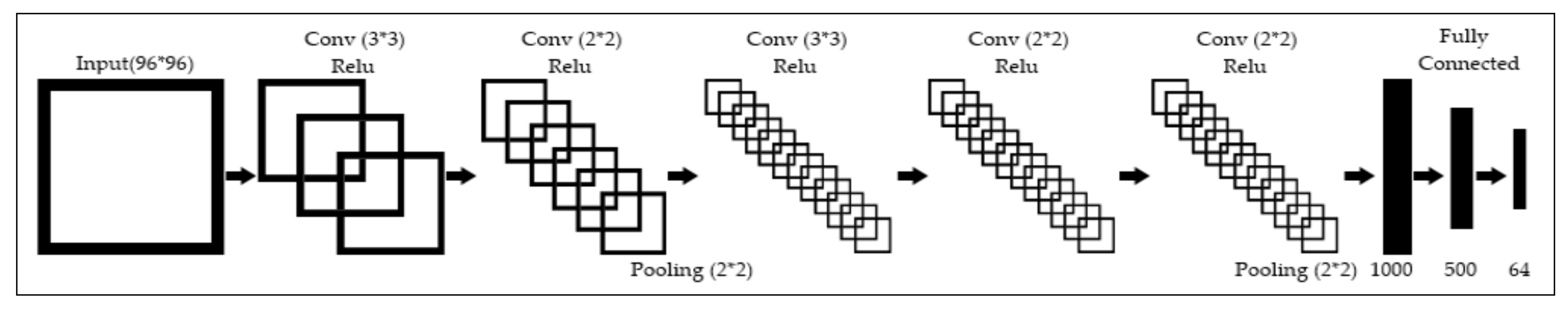
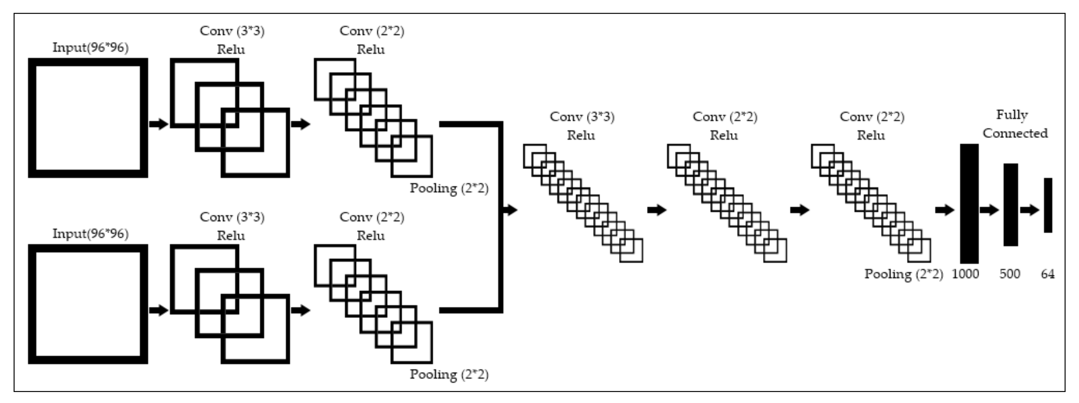
We record at the Kinect’s maximum capabilities, RGB ($1920\times 1080$) and Depth ($512\times 424$) at 30 fps, for speed we save both files in binary format. The images stored are unmodified from the ones received from the Kinect, no lossy compression is implemented. As the data is stored in raw binary format the dataset requires, at the time of writing, over 675 GB of storage for the full dataset.

3.2. Methodology

We implement multiple near-identical networks that function by pre-processing the image with convolutions with Rectified Linear Unit (ReLU) activations and then a series of fully connected layers to determine the final output. We illustrate the base networks in Figure 2. The base networks take a single stream of data, Gs, RGB or Depth and process through a series of convolutions to extract facial features. We use max-pooling to focus on high level features, and decrease processing requirements, but take into consideration that this can negatively impact accuracy [32]. The network utilises ReLU as an activation function after each convolutional layer as it does not normalise data. The resulting feature maps are then processed by fully connected layers to predict the facial landmarks. For the second stage, we examine the effectiveness of merging data streams, RGBD and GsD, we have a multiple input model, shown in Figure 3. The merge network used two CNNs: one to take the RGB/ Gs image; and another to take the Depth image. The two networks then use a series of convolutions to extract unique features from each of the inputs. The results of the two CNNs are combined and used as input to a third network. The third network further convolutes over the images giving a high value feature set for the fully connected layer.

As auxiliary features do affect how the network learns and XYZ points are desired, but not commonly predicted, we repeat the experiments not just with different data streams, but alternative outputs. The different outputs aid in showing how the networks can understand and learn both the features and facial structure, in different spaces. The three types of outputs and their metrics that we train the networks to predict are:

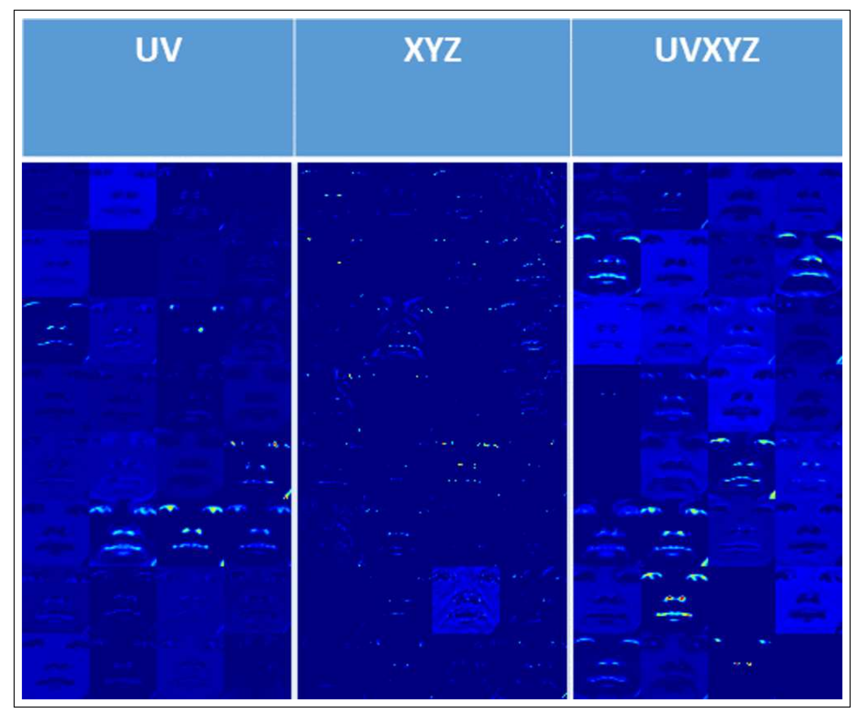
• The UV coordinates, in pixels
• The XYZ coordinates, in meters
• The UVXYZ coordinates

Where the UV points are the 2D image landmark coordinates and the XYZ points are the 3D location of the landmarks in camera space. As the outputs are in non-compatible metrics, they cannot be predicted in the same fully connect layer. To overcome this, we propose a multi-model output, where the final convolutional outputs are fed into different output models. This means, for UV and XYZ, there will be one model of fully connected layers for the convolution to be passed into. However, the UVXYZ network will have the convolutions output into two different models, one for UV calculation and one for XYZ. Traditionally with the Kinect, we require the 2D landmarks and use them to reconstruct the 3D points with a Depth map. Furthermore, by asking a network to infer UV and XYZ points, it could adopt the similar methodology, thus improving performance.

The networks are trained with a batch size of 240 using a stride of one over 100 epochs, using tensor-flow [33] with the Keras [34] API. We used the KOED dataset with 10-fold cross-validation; this ensures the network is trained, validated and tested on multiple participants, illustrating reliability. The cross-validation split was performed semi-randomly, with 70% training, 20% validation and 10% testing, ensuring no participant existed in multiple sets. We use MSE as our loss function, shown in Equation (1), using Adam [35] as the optimiser. MSE has more emphasises on large numbers allowing for large outliers to be resolved during training. However, we also calculate the MAE, as shown in Equation (2). MAE gives equal weight to all the errors illustrating the overall error. By using these error functions, we can determine the number of errors the networks produce and the size of errors. We use MSE for training as it is traditional in regression-based deep learning.

$$\mathrm{MSE}=\sum _{i=0}^n\frac{(y_i-y_i^{\prime })}{n}$$

(1)

where:

• n is the number of samples in the training batches.
• $y_i$ is the ground truth for the training image.
• $y_i^{\prime }$ is the predicted output for the training image.

$$\mathrm{MAE}=\sum _{i=0}^n\frac{|y_i-y_i^{\prime }|}{n}$$

(2)

where:

• n is the number of samples in the training batches.
• $y_i$ is the ground truth for the training image.
• $y_i^{\prime }$ is the predicted output for the training image.

4. Results

To compare the networks, we first show the validation during training and examine the performance of each stream. For each of the results we start with the UV (2D), then XYZ (3D) and finally, the UV XYZ (All) results. After this, we show an evaluation of the networks on testing data and the feature maps produced by the networks. Finally, we examine the results of the testing set with both MSE and MAE scores.

Figure 4 illustrates that for the prediction of UV landmarks, both RGB and Gs converge at similar epochs, 40. In addition, they both share many similar traits, such as that they both start with a significantly lower loss and have more stable learning than input streams that incorporate Depth. Overall, RGB performs the best in both MSE and MAE. The networks that merge visual and Depth data converge much later than RGB and Gs, but their results of MSE are close to the RGB and Gs scores. RGBD and GsD have unstable learning curves and encounter hidden gradients that cause loss to increase rapidly. The single channel GsD converges earlier than RGBD, indicating that a single clean frame learns faster on how to smooth a noisy Depth map than a three channel RGB image. The single channel Depth encounters the most unstable learning and converges at a much later stage, showing without a visual stream to assist the Depth data cannot easily locate UV landmarks. Furthermore, this is illustrated by Depth performing the worst when evaluated on MSE and MAE.

Figure 5 illustrates the MSE of the XYZ only network, like UV, RGB and Gs start with a low loss and converge the quickest at around epoch 30. However, the learning is unstable, indicating retrieving accurate 3D landmarks from visual images is a difficult task, although in the final epoch RGB has the lowest MSE. The input streams that incorporate Depth converge sooner than in the UV prediction networks. Furthermore, their learning rate is more stable than the RGB and Gs stream, but hidden gradients are still an issue. In addition, they converge at a similar location slightly higher than RGB and Gs, although at some point they score lower loss than the RGB and Gs networks. This convergence also occurs after a hidden gradient, indicating there is a shared local minimum caused by the inclusion of Depth data, the most prominent of these is GsD, which consistently has the lowest loss over epochs until it reaches a hidden gradient, to which it then becomes the worst performing stream.

Figure 6 illustrates the MSE of the UVXYZ networks, where RGB and Gs begin with the lowest loss, but RGB has a significantly lower loss than Gs. The learning rates of RGB and Gs are stable and converge quickly around epoch 43, with Gs performing the best. The input streams that incorporate Depth data also converge quickly, with Depth and GsD having stable learning rates, unlike RGBD. Furthermore, hidden gradients are still an issue. However, unlike in UV and XYZ only networks, the UVXYZ quickly recovers. This demonstrates how auxiliary information is benefiting the networks ability to learn from the different data streams by overcoming issues, such as the local minimum seen in Figure 5.

Figure 7 visually compares the results in both 2D and 3D. We summarise the observations:

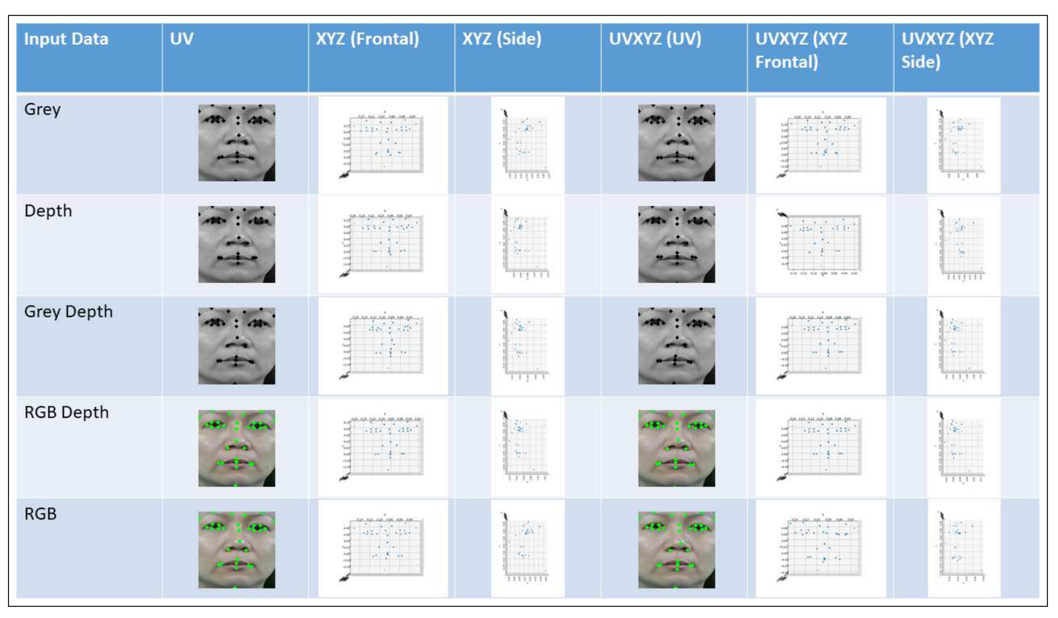
• In the UV only prediction, the results are visually similar, but there is some deviation between each of the networks. When using Depth as the input stream, the predictions of both the right eye and lip corners are predicted less precise than the other input streams; this could be directly affected by the noise in the Depth maps, as when merged with a visual stream, performance is improved.
• For UVXYZ, there is no noticeable difference between the UV results.
• For the XYZ only predictions we see much larger discriminations in the predicted facial landmarks. Some of the major changes are:

  -

  From the frontal view there is a variation in the mouth width, with Gs being the smallest and Depth being the widest.

  -

  Nose landmarks shifts in GsD were the nose tip and right nostril are predicted close to each other.

  -

  Eye shape changes between networks, Gs and RGBD produce round smooth eyes. Whereas others are more jagged and uneven.

  -

  From the side view, we see the profile of the face change with the forehead and nose shape varying greatly between networks.

• In contrast to the UV results in the UVXYZ network, with the addition of auxiliary information the resulting geometric landmarks on the mouth, nose, eye and eyebrows, become more precise and consistent. In most of the cases the eyes are smoother, the eyebrows are more evenly spaced, the nose irregularity in GsD no longer occurs and the mouth width consistency has improved greatly. These results show that, as UV is easier for the networks to learn as all streams manage similar results, when used as auxiliary information, they aid to standardise the 3D locations as well. However, there are still some variations in the profile of the nose and in RGB the right eye is predicted to be shut.

As shown in

Table 1. Table of the testing set evaluation on MSE. Bold highlights the lowest error.

Input Data	UV MSE	XYZ MSE	UVXYZ MSE (Combined)	UVXYZ MSE (UV)	UVXYZ MSE (XYZ)
Gs	1.8192	0.0023	1.3695	1.3676	0.0019
Depth	6.4672	0.0023	6.6509	6.6482	0.0027
Gs Depth	2.1845	0.0022	1.8933	1.8911	0.0022
RGB Depth	2.1561	0.0022	2.8744	2.8752	0.0022
RGB	1.7488	0.0023	1.5612	1.5592	0.0019

, for UV landmarks RGB has the lowest MSE, with Gs not far behind. It also shows that for predicting landmarks in 3D only, that having both a visual and Depth data allows for the highest precision results, with RGBD and GsD scoring the lowest with marginal differences in score. For the MAE and MSE of the UVXYZ networks, we show the separate stages of the loss calculation:

• Combined loss, which is the sum of UV and XYZ layers loss.
• UV loss, the loss of the UV layers alone.
• XYZ loss, the loss of the XYZ layers alone.

The combined loss shows the overall network performance, but the UV and XYZ alone show the networks’ performance on the individual outputs. By comparing the loss of the UV and XYZ alone, we illustrate how the auxiliary information is affecting network performance, compared to networks predicting UV only or XYZ only landmarks. When trying to predict UVXYZ data, Gs performs the best overall. We show that by introducing the 3D landmarks, we reduce the overall loss significantly to UV alone in both RGB, Gs and GsD networks. Furthermore, the prediction of XYZ is improved in the same networks. We see similar results in the MAE, shown in

Table 2. Table of the testing set evaluation on MAE. Bold highlights the lowest error.

Input Data	UV MAE	XYZ MAE	UVXYZ MAE (Combined)	UVXYZ MAE (UV)	UVXYZ MAE (XYZ)
Gs	1.0052	0.0341	0.9127	0.8797	0.0330
Depth	1.9150	0.0361	1.9705	1.9322	0.0382
Gs Depth	1.1210	0.0379	1.0617	1.0246	0.0371
RGB Depth	1.0848	0.0367	1.3056	1.2685	0.0371
RGB	0.9553	0.0346	0.9685	0.9388	0.0297

, where networks reduce the loss below the UV alone networks. However, RGB sees the least MAE for UV. For overall combined loss and XYZ loss, Gs scores the lowest in MSE and MAE.

The key differences in single task networks and multi-task networks in predicting facial landmarks were observed in the feature maps of the networks, illustrated in Figure 8. The network kernels learned the spatial information from UV prediction. Therefore, the feature maps shown in the UV prediction demonstrate the activation of appearance-based facial features. On the other hand, when predicting the geometry coordinate of XYZ, we observed that the feature maps of the convolutional layers had point-based (facial landmarks) activation. This is due to the Z component which makes the facial landmarks more separable. The UVXYZ column depicts the features maps in UVXYZ prediction. We observed it has better pattern representation with both appearance based and point/landmarks information. The Gs network performs the best with the feature maps demonstrating the networks can process the input stream to focus on the specific landmark regions of the face. Further advantages occur when auxiliary information is added: the kernels become refined and are able to detect features with high intensity, as the network is forced to learn how the structure appears in both 2D and 3D. It also means the network can process the data more efficiently as the input is a single stream. However, a disadvantage of this system is that the image must be pre-processed from RGB to Gs.

To demonstrate the effectiveness of the network, we visualise the predicted landmarks of the Gs network on a 3D model, shown in Figure 9 (see Supplementary Materials). With Gs as input data stream, our proposed method predicts accurate 3D facial landmarks on raw Depth data using auxiliary information. Furthermore, this illustrates the accuracy of the network, even with raw Depth data, our proposed method manages to estimate accurate 3D facial landmarks after pre-processing to crop and resize Depth images for the network, where a human would be incapable of without full-size Depth images [36]. However, due to the noise from the raw data, the limitation of our proposed method is not able to locate the Z position precisely in some cases.

5. Discussion and Conclusions

In this work we have shown and illustrated the effect of different data streams within neural networks, to identify which streams are ideal for current research topics, as current literature uses a mixture. We also extended the work by the prediction of points in the camera (XYZ) space as this is a valuable resource in facial expression recognition and animation synthesis, but current literature focuses on image (UV) space coordinate systems. Unique insights into each stream of data were obtained, demonstrating the pros and cons of each stream. To prevent bias, an in-house dataset was used, showing that each network could reliably track facial features and expressions in both 2D and 3D. The networks showed that the existing data-streams could accurately predict 2D and 3D landmarks.

Comparing the results and feature maps of the networks demonstrates the ability of the networks to process and understand the different forms of data and if they are beneficial to the network. Full RGB performed the most effectively on UV with the least amount of errors and the lowest scale of errors. While Depth shows its effectiveness at predicting landmarks, the noise it presents requires additional streams, such as RGB to smooth out and retrieve reliable results. In the final experiment, for predicting UVXYZ, we show that although for UV alone RGB is the most efficient, Gs outperformed it, illustrating that more generalizable single frames are more effective when predicting a wide range of values. While Depth has shown to be difficult for the networks to learn from, with limitations such as exploding gradients, even after merging with cleaner streams it has been shown to be effective even when cropped and resized for the prediction of landmarks, where traditional methods require full-size Depth images.

This work focused exclusively on the use of neural networks to predict facial landmarks without the aid of physical markers, sensors, or reference points placed on the individuals. There have been many incremental studies into the use of neural networks to predict the image (UV) space landmarks successfully. However, the results all use different streams of data with little consensus on why the stream is used, except for dataset or memory limitations. In addition, XYZ coordinates are not being predicted by neural networks in current systems. For networks, many industries desire the use of 3D landmarks in real-time.

There are several limitations in this study, mostly related to the data used to train the network and the difficulty of 3D landmarks. Firstly, due to the context issue of cropping, a Depth map recording was done in a controlled environment, so the network must only learn a manageable part of the 3D viewing frustum. This, regarding animation, has an advantage as it normalises the facial position, while still tracking 3D facial movement. However, for full 3D prediction full Depth maps would still be required. Future work should seek out new technologies, such as the Intel real-sense [37], which could resolve the noise issue of the Kinect as it provides both higher resolution and cleaner Depth maps as shown by Carfagni et al. [38], which would aid the networks’ ability to learn from the data. Other aspects would be to further the work with a larger dataset to test the reliability of no Depth streams with a wider demographic of faces.

We have shown and analysed how the input data stream can affect a deep neural network framework, for the analysis of facial features, which can have an impact on facial recognition, reconstruction, animation, and security, by providing how the networks interact with the different data streams. The stream shows different levels of accuracy and reliability which can positively affect future work. Future work will include increasing the number of participants and increasing the amount of reliably tracked landmarks without marker 3D reference points on the face, as current literature is limited in this area.

6. Materials and Methods

We provide access to all codes used to build and train models on GitHub. We also provide demo codes to enable the real-time use of the trained models, with the use of a Kinect. All scripts are provided in python. The in-house KOED dataset will be made publicly available. However, in its raw form, the dataset requires over 675 GB to store at the time of writing, without any annotations.

References

1. Vicon Motion Systems Ltd. Capture Systems; Vicon Motion Systems Ltd.: Oxford, UK, 2016. [Google Scholar]
2. Zhang, K.; Zhang, Z.; Li, Z.; Qiao, Y. Joint Face Detection and Alignment Using Multitask Cascaded Convolutional Networks. IEEE Signal Process. Lett. 2016, 23, 1499–1503. [Google Scholar] [CrossRef]
3. Ranjan, R.; Patel, V.M.; Chellappa, R. HyperFace: A Deep Multi-task Learning Framework for Face Detection, Landmark Localization, Pose Estimation, and Gender Recognition. IEEE Trans. Pattern Anal. Mach. Intell. 2016, 1. [Google Scholar] [CrossRef]
4. Bui, H.M.; Lech, M.; Cheng, E.; Neville, K.; Burnett, I.S. Using grayscale images for object recognition with convolutional-recursive neural network. In Proceedings of the 2016 IEEE Sixth International Conference on Communications and Electronics (ICCE), Ha Long, Vietnam, 27–29 July 2016; pp. 321–325. [Google Scholar] [CrossRef]
5. Zhou, E.; Fan, H.; Cao, Z.; Jiang, Y.; Yin, Q. Extensive facial landmark localization with coarse-to-fine convolutional network cascade. In Proceedings of the 2013 IEEE International Conference on Computer Vision Workshops, Sydney, NSW, Australia, 2–8 December 2013; pp. 386–391. [Google Scholar] [CrossRef]
6. Jourabloo, A.; Liu, X. Large-Pose Face Alignment via CNN-Based Dense 3D Model Fitting. In Proceedings of the 2016 IEEE Conference on Computer Vision and Pattern Recognition (CVPR), Las Vegas, NV, USA, 27–30 June 2016; pp. 4188–4196. [Google Scholar] [CrossRef]
7. Han, X.; Yap, M.H.; Palmer, I. Face recognition in the presence of expressions. J. Softw. Eng. Appl. 2012, 5, 321. [Google Scholar] [CrossRef]
8. Faceware Technologies Inc. Faceware; Faceware Technologies Inc: Sherman Oaks, CA, USA, 2015. [Google Scholar]
9. Feng, Z.H.; Kittler, J. Advances in facial landmark detection. Biom. Technol. Today 2018, 2018, 8–11. [Google Scholar] [CrossRef]
10. Phillips, P.J.; Flynn, P.J.; Scruggs, T.; Bowyer, K.W.; Chang, J.; Hoffman, K.; Marques, J.; Min, J.; Worek, W. Overview of the Face Recognition Grand Challenge. In Proceedings of the 2005 IEEE Computer Society Conference on Computer Vision and Pattern Recognition (CVPR’05), San Diego, CA, USA, 20–25 June 2005; IEEE Computer Society: Washington, DC, USA, 2005; Volume 1, pp. 947–954. [Google Scholar] [CrossRef]
11. Microsoft. Microsoft Kinect; Microsoft: Redmond, WA, USA, 2013. [Google Scholar]
12. Zhang, Z.; Luo, P.; Loy, C.C.; Tang, X. Facial landmark detection by deep multi-task learning. In Lecture Notes in Computer Science; (Including Subseries Lecture Notes in Artificial Intelligence and Lecture Notes in Bioinformatics); Springer: Berlin, Germany, 2014; Volume 8694, pp. 94–108. [Google Scholar]
13. Hand, E.M.; Chellappa, R. Attributes for Improved Attributes: A Multi-Task Network for Attribute Classification. arXiv, 2016; arXiv:1604.07360. [Google Scholar]
14. Zhang, Z.; Luo, P.; Loy, C.C.; Tang, X. Learning Deep Representation for Face Alignment with Auxiliary Attributes. IEEE Trans. Pattern Anal. Mach. Intell. 2016, 38, 918–930. [Google Scholar] [CrossRef] [PubMed]
15. Sun, Y.; Wang, X.; Tang, X. Deep convolutional network cascade for facial point detection. In Proceedings of the IEEE Computer Society Conference on Computer Vision and Pattern Recognition, Portland, OR, USA, 23–28 June 2013; pp. 3476–3483. [Google Scholar] [CrossRef]
16. Lai, H.; Xiao, S.; Pan, Y.; Cui, Z.; Feng, J.; Xu, C.; Yin, J.; Yan, S. Deep Recurrent Regression for Facial Landmark Detection. arXiv, 2015; arXiv:1510.09083. [Google Scholar] [CrossRef]
17. Hochreiter, S.; Schmidhuber, J. Long short-term memory. Neural Comput. 1997, 9, 1735–1780. [Google Scholar] [CrossRef] [PubMed]
18. Liu, H.; Lu, J.; Feng, J.; Zhou, J. Learning Deep Sharable and Structural Detectors for Face Alignment. IEEE Trans. Image Process. 2017, 26, 1666–1678. [Google Scholar] [CrossRef] [PubMed]
19. Angeline, P.J.; Angeline, P.J.; Saunders, G.M.; Saunders, G.M.; Pollack, J.B.; Pollack, J.B. An evolutionary algorithm that constructs recurrent neural networks. IEEE Trans. Neural Netw. 1994, 5, 54–65. [Google Scholar] [CrossRef] [PubMed]
20. Dibeklioglu, H.; Salah, A.A.; Akarun, L. 3D Facial Landmarking under Expression, Pose, and Occlusion Variations. In Proceedings of the 2008 IEEE Second International Conference on Biometrics: Theory, Applications and Systems, Arlington, VA, USA, 29 September–1 October 2008; pp. 3–8. [Google Scholar]
21. Nair, P.; Cavallaro, A. 3-D Face Detection, Landmark Localization, and Registration Using a Point Distribution Model. IEEE Trans. Multimed. 2009, 11, 611–623. [Google Scholar] [CrossRef]
22. Ngiam, J.; Khosla, A.; Kim, M.; Nam, J.; Lee, H.; Ng, A.Y. Multimodal Deep Learning. In Proceedings of the 28th International Conference on Machine Learning (ICML), Orlando, FL, USA, 3–7 November 2014; pp. 689–696. [Google Scholar] [CrossRef]
23. Park, E.; Han, X.; Tamara, L.; Berg, A.C. Combining Multiple Sources of Knowledege in Deep CNNs for Action Recognition. In Proceedings of the 2016 IEEE Winter Conference on Applications of Computer Vision (WACV), Lake Placid, NY, USA, 7–9 March 2016; pp. 1–8. [Google Scholar]
24. Socher, R.; Huval, B. Convolutional-recursive deep learning for 3D object classification. In Advances in Neural Information Processing Systems 9: Proceedings of the 1996 Conference; MIT Press Ltd.: Cambridge, MA, USA, 2012; pp. 1–9. [Google Scholar]
25. Liu, L.; Shao, L. Learning discriminative representations from RGB-D video data. IJCAI 2013, 1, 1493. [Google Scholar]
26. Cao, C.; Weng, Y.; Zhou, S.; Tong, Y.; Zhou, K. FaceWarehouse: A 3D facial expression database for visual computing. IEEE Trans. Vis. Comput. Graph. 2014, 20, 413–425. [Google Scholar] [CrossRef] [PubMed]
27. Microsoft. Microsoft Kinect 360; Microsoft: Redmond, WA, USA, 2010. [Google Scholar]
28. Fanelli, G.; Dantone, M.; Gall, J.; Fossati, A.; Van Gool, L. Random Forests for Real Time 3D Face Analysis. Int. J. Comput. Vis. 2013, 101, 437–458. [Google Scholar] [CrossRef]
29. Min, R.; Kose, N.; Dugelay, J.L. KinectFaceDB: A Kinect Face Database for Face Recognition. IEEE Trans. Syst. Man Cybern. A 2014, 44, 1534–1548. [Google Scholar] [CrossRef]
30. Hg, R.I.; Jasek, P.; Rofidal, C.; Nasrollahi, K.; Moeslund, T.B.; Tranchet, G. An RGB-D database using microsoft’s kinect for windows for face detection. In Proceedings of the 2012 8th International Conference on Signal Image Technology and Internet Based Systems, (SITIS’2012), Naples, Italy, 25–29 November 2012; pp. 42–46. [Google Scholar] [CrossRef]
31. Erdogmus, N.; Marcel, S. Spoofing in 2D face recognition with 3D masks and anti-spoofing with Kinect. In Proceedings of the 2013 IEEE 6th International Conference on Biometrics: Theory, Applications and Systems (BTAS), Arlington, VA, USA, 29 September–2 October 2013. [Google Scholar] [CrossRef]
32. Kendrick, C.; Tan, K.; Walker, K.; Yap, M.H. The Application of Neural Networks for Facial Landmarking on Mobile Devices. In Proceedings of the 13th International Joint Conference on Computer Vision, Imaging and Computer Graphics Theory and Applications (VISAPP), Funchal, Portugal, 27–29 January 2018; INSTICC/SciTePress: Setúbal, Portugal, 2018; Volume 4, pp. 189–197. [Google Scholar] [CrossRef]
33. Abadi, M.; Barham, P.; Chen, J.; Chen, Z.; Davis, A.; Dean, J.; Devin, M.; Ghemawat, S.; Irving, G.; Isard, M.; et al. TensorFlow: A System for Large-Scale Machine Learning. Osdi 2016, 16, 265–283. [Google Scholar]
34. Chollet, F. Keras. 2016. Available online: https://keras.io/ (accessed on 15 June 2018).
35. Kingma, D.P.; Ba, J.L. Adam: A Method for Stochastic Optimization. arXiv, 2015; arXiv:1412.6980v8. [Google Scholar]
36. Kendrick, C.; Tan, K.; Williams, T.; Yap, M.H. An Online Tool for the Annotation of 3D Models. In Proceedings of the 2017 12th IEEE International Conference on Automatic Face & Gesture Recognition (FG 2017), Washington, DC, USA, 30 May–3 June 2017; pp. 362–369. [Google Scholar] [CrossRef]
37. Intel. RealSense SR300; Intel: Santa Clara, CA, USA, 2016. [Google Scholar]
38. Carfagni, M.; Furferi, R.; Governi, L.; Servi, M.; Uccheddu, F.; Volpe, Y. On the Performance of the Intel SR300 Depth Camera: Metrological and Critical Characterization. IEEE Sens. J. 2017, 17, 4508–4519. [Google Scholar] [CrossRef]
Article Metrics
Citations
Article Access Statistics
Multiple requests from the same IP address are counted as one view.