Bayer Image Demosaicking Using Eight-Directional Weights Based on the Gradient of Color Difference


Abstract
1. Introduction
2. Related Work
2.1. The Outline of R/B Interpolation in MLRI
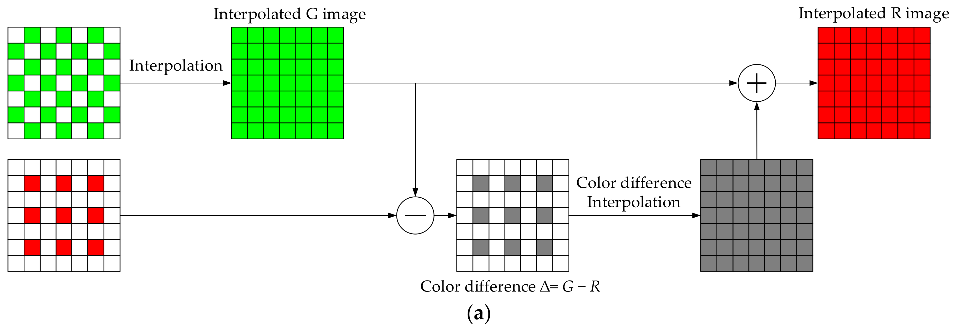
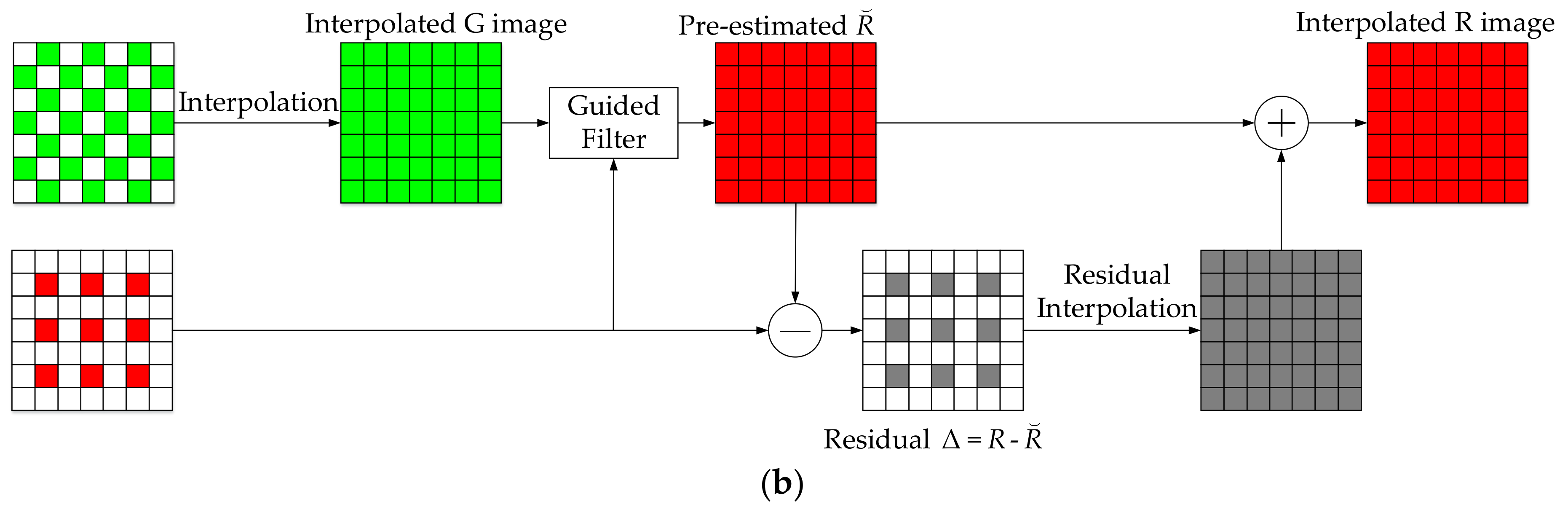
2.1.1. Color Difference Interpolation and Residual Interpolation
2.1.2. Laplacian Energy
2.1.3. The Guide Filter in MLRI
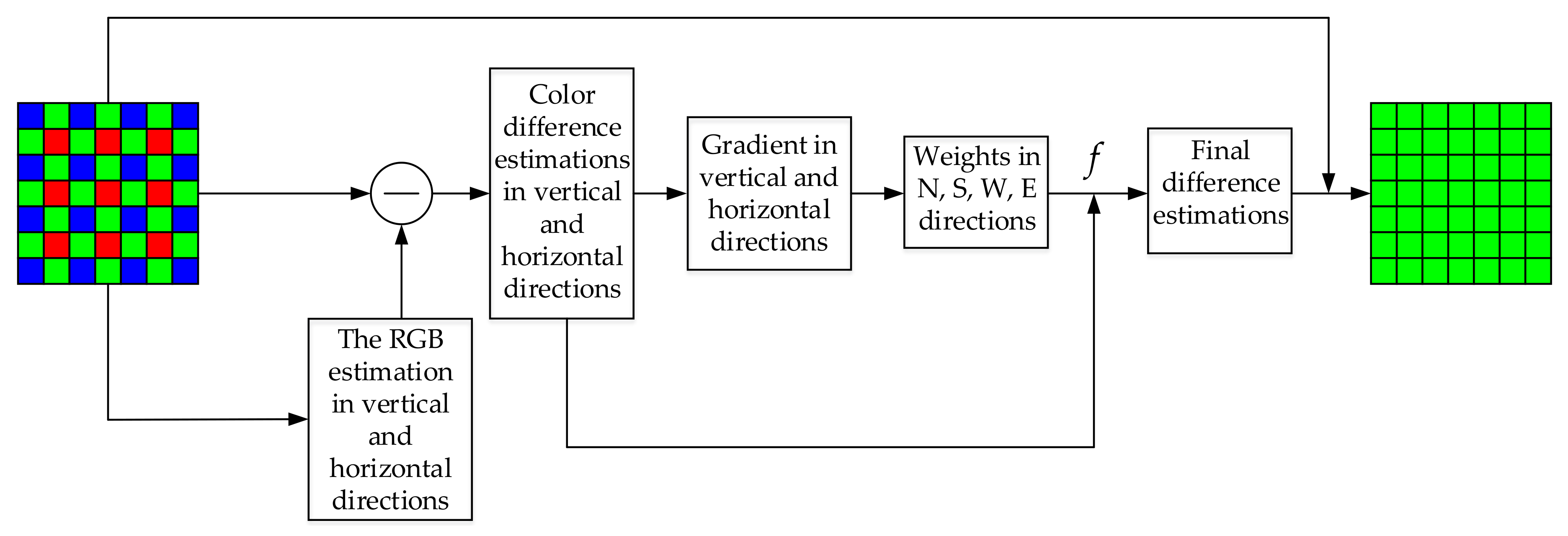
2.2. The Outline of G Interpolation in GBTF and MDWI-GF
3. The Proposed Algorithm
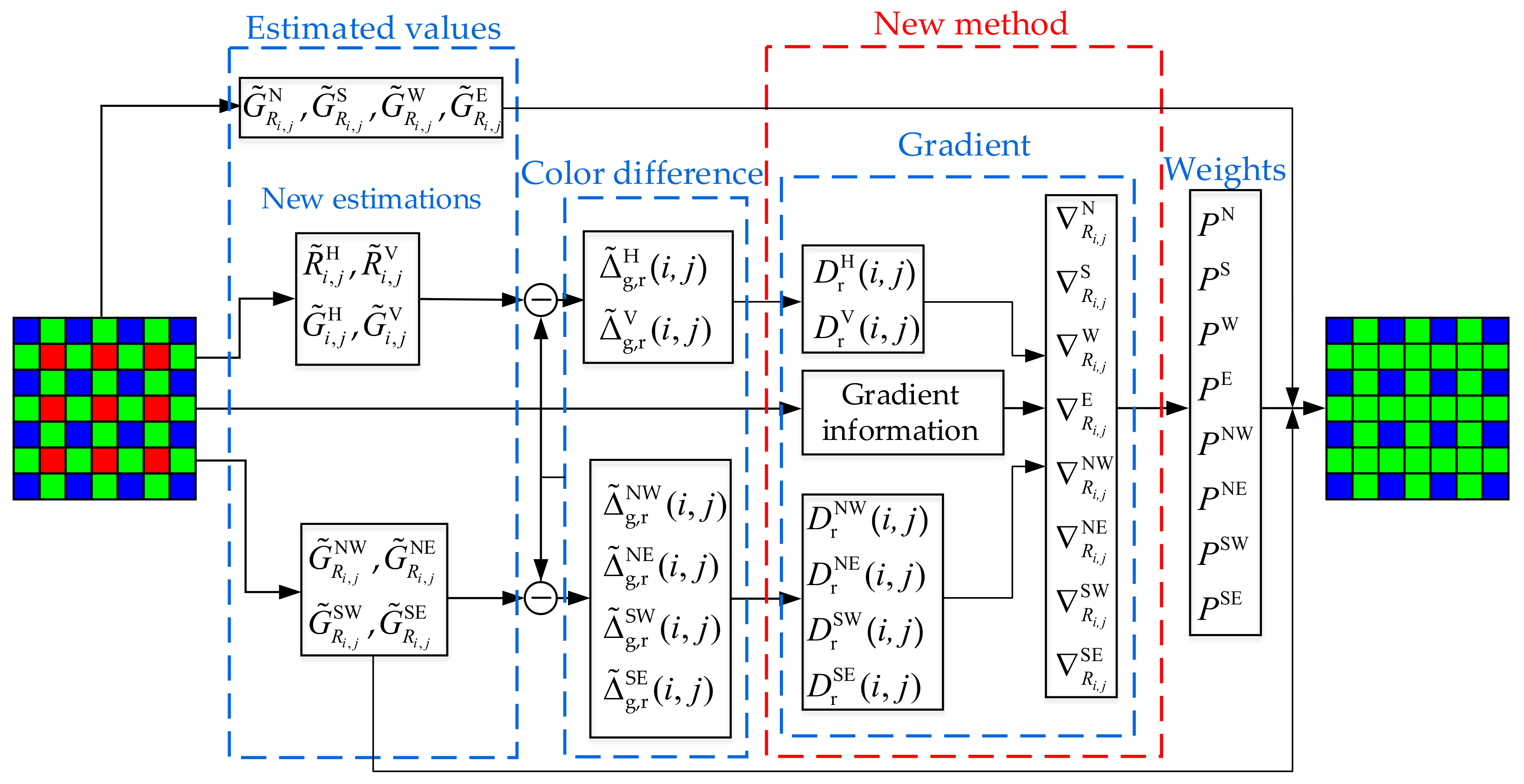
3.1. The Outline of Proposed Algorithm
3.2. The Interpolation of G Values
4. Experimental Results and Discussions
5. Conclusions
Author Contributions
Acknowledgments
Conflicts of Interest
References
- Wang, D.Y.; Yu, G.; Zhou, X.; Wang, C.Y. Image Demosaicking for Bayer-Patterned CFA Images Using Improved Linear Interpolation. In Proceedings of the 7th International Conference on Information Science and Technology, Da Nang, Vietnam, 16–19 April 2017; pp. 464–469. [Google Scholar]
- Zhang, L.; Wu, X. Color demosaicking via directional linear minimum mean square-error estimation. IEEE Trans. Image Process. 2005, 14, 2167–2178. [Google Scholar] [CrossRef] [PubMed]
- Zhang, L.; Wu, X.; Buades, A.; Li, X. Color demosaicking by local directional interpolation and nonlocal adaptive thresholding. J. Electron. Imaging 2011, 20, 16. [Google Scholar]
- Wu, J.; Anisetti, M.; Wu, W.; Damiani, E.; Jeon, G. Bayer demosaicking with polynomial interpolation. IEEE Trans. Image Process. 2016, 25, 5369–5382. [Google Scholar] [CrossRef] [PubMed]
- Chen, W.-J.; Chang, P.-Y. Effective demosaicking algorithm based on edge property for color filter arrays. Digit. Signal Process. 2012, 22, 163–169. [Google Scholar] [CrossRef]
- Chung, K.-H.; Chan, Y.-H. Low-complexity color demosaicing algorithm based on integrated gradients. J. Electron. Imaging 2010, 19, 15. [Google Scholar] [CrossRef]
- Pekkucuksen, I.; Altunbasak, Y. Edge strength filter based color filter array interpolation. IEEE Trans. Image Process. 2012, 21, 393–397. [Google Scholar] [CrossRef] [PubMed]
- Pekkucuksen, I.; Altunbasak, Y. Gradient Based Threshold Free Color Filter Array Interpolation. In Proceedings of the IEEE International Conference on Image Processing, Hong Kong, China, 26–29 September 2010; pp. 137–140. [Google Scholar]
- Wang, J.; Wu, J.; Wu, Z.; Jeon, G. Filter-based Bayer pattern CFA demosaicking. Circuits Syst. Signal Process. 2017, 36, 2917–2940. [Google Scholar] [CrossRef]
- Kiku, D.; Monno, Y.; Tanaka, M.; Okutomi, M. Residual interpolation for color image demosaicking. IEEE Tokyo Inst. Technol. 2013, 978, 2304–2308. [Google Scholar]
- He, K.; Sun, J.; Tang, X. Guided image filtering. IEEE Trans. Pattern Anal. Mach. Intell. 2013, 35, 1397–1409. [Google Scholar] [CrossRef] [PubMed]
- Kiku, D.; Monno, Y.; Tanaka, M.; Okutomi, M. Minimized-Laplacian Residual Interpolation for Color Image Demosaicking. In Proceedings of the SPIE, Digital Photography X, San Francisco, CA, USA, 3–5 February 2014; Volume 9023, pp. 1–8. [Google Scholar]
- Kiku, D.; Monno, Y.; Tanaka, M.; Okutomi, M. Beyond color difference: Residual interpolation for color image demosaicking. IEEE Trans. Image Process. 2016, 25, 1288–1300. [Google Scholar] [CrossRef] [PubMed]
- Ye, W.; Ma, K.K. Color image demosaicking using iterative residual interpolation. IEEE Trans. Image Process. 2015, 24, 5879–5891. [Google Scholar] [CrossRef] [PubMed]
- Kim, Y.; Jeong, J. Four-direction residual interpolation for demosaicking. IEEE Trans. Circuits Syst. Video Technol. 2016, 26, 881–890. [Google Scholar] [CrossRef]
- Monno, Y.; Kiku, D.; Tanaka, M.; Okutomi, M. Adaptive residual interpolation for color and multispectral image demosaicking. Sensors 2017, 17, 21. [Google Scholar] [CrossRef] [PubMed]
- Wang, L.; Jeon, G. Bayer pattern CFA demosaicking based on multi-directional weighted interpolation and guided filter. IEEE Signal Process. Lett. 2015, 22, 2083–2087. [Google Scholar] [CrossRef]
- Satya Prakash, V.N.V.; Satya Prasad, K.; Jaya Chandra Prasad, T. Demosaicing of color images by accurate estimation of luminance. Telkomnika 2016, 14, 47–55. [Google Scholar] [CrossRef]
- Ji, Y.K.; Sang, W.P.; Min, K.P.; Kang, M.G. Aliasing artifacts reduction with subband signal analysis for demosaicked images. Digit. Signal Process. 2016, 59, 115–128. [Google Scholar]
- Wu, J.; Timofte, R.; Gool, L.V. Demosaicing based on directional difference regression and efficient regression priors. IEEE Trans. Image Process. 2016, 25, 3862–3874. [Google Scholar] [CrossRef] [PubMed]
- Yang, B.; Luo, J.; Guo, L.; Cheng, F. Simultaneous image fusion and demosaicing via compressive sensing. Inf. Process. Lett. 2016, 116, 447–454. [Google Scholar] [CrossRef]


| Test Images | DLMMSE [2] | IG [6] | GBTF [8] | RI [10] | MLRI [12] | MDWI-GF [17] | Proposed |
|---|---|---|---|---|---|---|---|
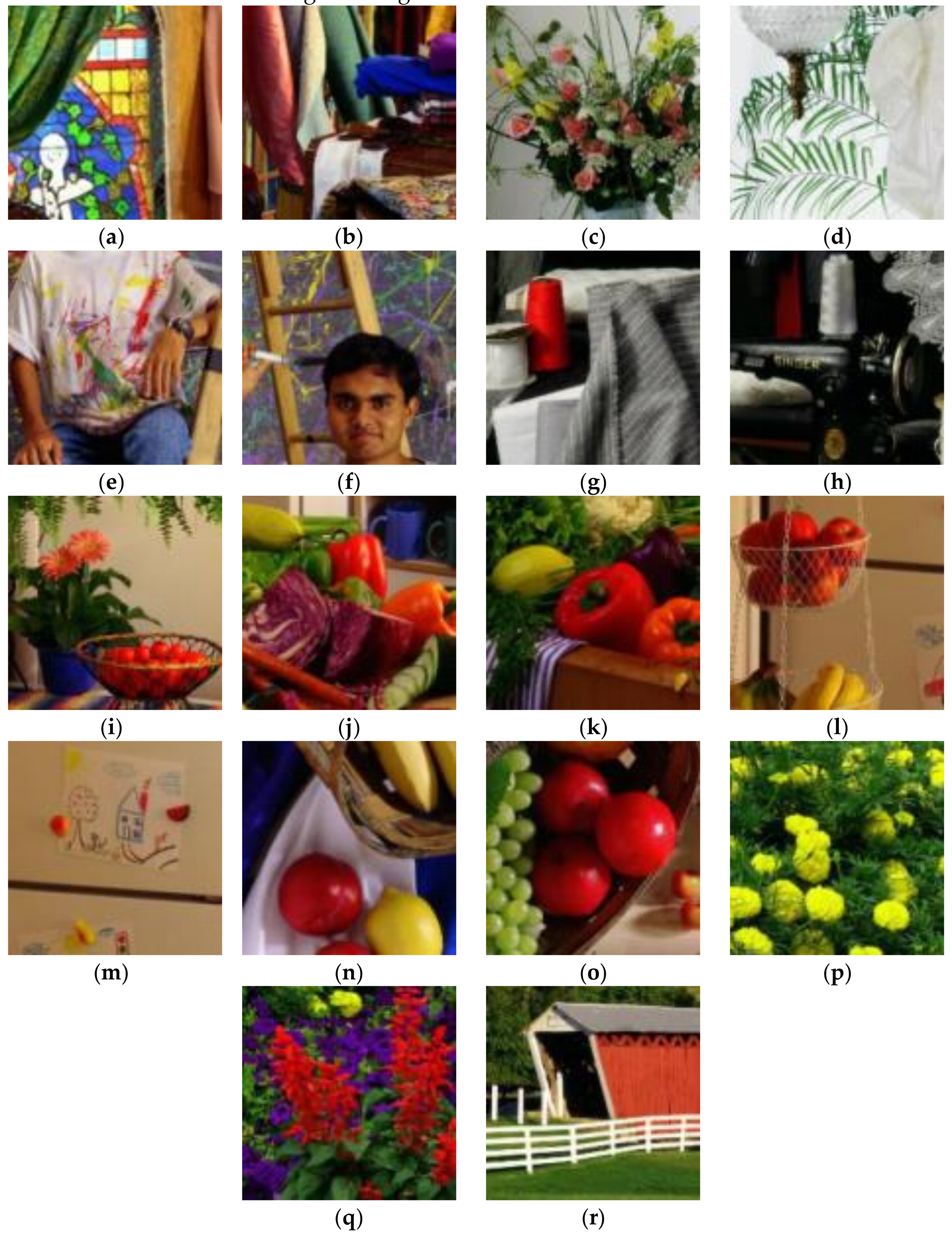
| Figure 9a | 26.98 | 28.52 | 26.89 | 28.89 | 28.98 | 29.23 | 29.36 |
| Figure 9b | 33.69 | 34.62 | 33.62 | 34.83 | 35.06 | 34.80 | 34.83 |
| Figure 9c | 32.59 | 32.63 | 32.69 | 33.80 | 33.85 | 32.58 | 32.48 |
| Figure 9d | 34.33 | 34.89 | 34.74 | 37.53 | 37.66 | 37.26 | 37.20 |
| Figure 9e | 31.28 | 33.25 | 30.92 | 33.47 | 33.94 | 34.25 | 34.41 |
| Figure 9f | 33.83 | 37.11 | 33.21 | 37.73 | 38.29 | 38.83 | 38.86 |
| Figure 9g | 38.65 | 36.80 | 38.97 | 37.62 | 37.50 | 35.31 | 35.18 |
| Figure 9h | 37.46 | 36.72 | 37.50 | 36.03 | 37.05 | 35.62 | 37.06 |
| Figure 9i | 34.41 | 35.48 | 34.31 | 35.71 | 36.49 | 36.62 | 37.10 |
| Figure 9j | 36.34 | 37.90 | 36.25 | 37.92 | 38.65 | 38.77 | 38.75 |
| Figure 9k | 37.24 | 39.30 | 37.04 | 39.40 | 39.98 | 39.99 | 39.85 |
| Figure 9l | 36.61 | 38.86 | 36.65 | 39.53 | 39.65 | 38.21 | 38.32 |
| Figure 9m | 38.80 | 40.10 | 38.65 | 40.07 | 40.63 | 40.56 | 40.61 |
| Figure 9n | 37.24 | 38.30 | 37.10 | 38.72 | 38.81 | 38.96 | 38.87 |
| Figure 9o | 37.27 | 38.35 | 37.09 | 38.17 | 38.92 | 39.12 | 39.15 |
| Figure 9p | 30.45 | 34.54 | 30.08 | 34.90 | 35.16 | 35.21 | 34.99 |
| Figure 9q | 29.31 | 31.07 | 29.02 | 31.77 | 32.58 | 33.15 | 33.48 |
| Figure 9r | 33.90 | 35.49 | 34.04 | 36.48 | 36.12 | 35.54 | 35.57 |
| Average | 34.47 | 35.77 | 34.38 | 36.25 | 36.63 | 36.33 | 36.45 |
| Test Images | DLMMSE [2] | IG [6] | GBTF [8] | RI [10] | MLRI [12] | MDWI-GF [17] | Proposed |
|---|---|---|---|---|---|---|---|
| Figure 9a | 0.9791 | 0.9882 | 0.9852 | 0.9891 | 0.9899 | 0.9905 | 0.9910 |
| Figure 9b | 0.9910 | 0.9958 | 0.9962 | 0.9970 | 0.9969 | 0.9968 | 0.9970 |
| Figure 9c | 0.9945 | 0.9944 | 0.9951 | 0.9967 | 0.9962 | 0.9966 | 0.9965 |
| Figure 9d | 0.9958 | 0.9968 | 0.9967 | 0.9990 | 0.9984 | 0.9988 | 0.9987 |
| Figure 9e | 0.9937 | 0.9964 | 0.9957 | 0.9975 | 0.9976 | 0.9977 | 0.9979 |
| Figure 9f | 0.9895 | 0.9954 | 0.9939 | 0.9963 | 0.9968 | 0.9969 | 0.9971 |
| Figure 9g | 0.9990 | 0.9981 | 0.9990 | 0.9986 | 0.9988 | 0.9987 | 0.9985 |
| Figure 9h | 0.9980 | 0.9957 | 0.9976 | 0.9972 | 0.9980 | 0.9980 | 0.9976 |
| Figure 9i | 0.9939 | 0.9965 | 0.9966 | 0.9979 | 0.9978 | 0.9979 | 0.9982 |
| Figure 9j | 0.9883 | 0.9970 | 0.9968 | 0.9981 | 0.9980 | 0.9981 | 0.9984 |
| Figure 9k | 0.9886 | 0.9965 | 0.9971 | 0.9979 | 0.9979 | 0.9978 | 0.9982 |
| Figure 9l | 0.9907 | 0.9983 | 0.9997 | 0.9990 | 0.9990 | 0.9993 | 0.9996 |
| Figure 9m | 0.9941 | 0.9989 | 0.9991 | 0.9994 | 0.9993 | 0.9992 | 0.9994 |
| Figure 9n | 0.9886 | 0.9979 | 0.9980 | 0.9986 | 0.9987 | 0.9984 | 0.9988 |
| Figure 9o | 0.9906 | 0.9974 | 0.9980 | 0.9982 | 0.9986 | 0.9983 | 0.9987 |
| Figure 9p | 0.9821 | 0.9940 | 0.9918 | 0.9956 | 0.9956 | 0.9959 | 0.9964 |
| Figure 9q | 0.9691 | 0.9784 | 0.9818 | 0.9874 | 0.9879 | 0.9885 | 0.9898 |
| Figure 9r | 0.9925 | 0.9968 | 0.9970 | 0.9982 | 0.9979 | 0.9977 | 0.9977 |
| Average | 0.9899 | 0.9951 | 0.9953 | 0.9968 | 0.9968 | 0.9970 | 0.9972 |
© 2018 by the authors. Licensee MDPI, Basel, Switzerland. This article is an open access article distributed under the terms and conditions of the Creative Commons Attribution (CC BY) license (http://creativecommons.org/licenses/by/4.0/).
Share and Cite
Liu, Y.; Wang, C.; Zhao, H.; Song, J.; Chen, S. Bayer Image Demosaicking Using Eight-Directional Weights Based on the Gradient of Color Difference. Symmetry 2018, 10, 222. https://doi.org/10.3390/sym10060222
Liu Y, Wang C, Zhao H, Song J, Chen S. Bayer Image Demosaicking Using Eight-Directional Weights Based on the Gradient of Color Difference. Symmetry. 2018; 10(6):222. https://doi.org/10.3390/sym10060222
Chicago/Turabian StyleLiu, Yizheng, Chengyou Wang, Hongming Zhao, Jiayang Song, and Shiyue Chen. 2018. "Bayer Image Demosaicking Using Eight-Directional Weights Based on the Gradient of Color Difference" Symmetry 10, no. 6: 222. https://doi.org/10.3390/sym10060222
APA StyleLiu, Y., Wang, C., Zhao, H., Song, J., & Chen, S. (2018). Bayer Image Demosaicking Using Eight-Directional Weights Based on the Gradient of Color Difference. Symmetry, 10(6), 222. https://doi.org/10.3390/sym10060222