Article

Exponential Aggregation Operator of Interval Neutrosophic Numbers and Its Application in Typhoon Disaster Evaluation

1
School of Economics and Management, Fuzhou University, Fuzhou 350116, China
2
College of Electronics and Information Science, Fujian Jiangxia University, Fuzhou 350108, China
3
Institute of Information Management, Fuzhou University, Fuzhou 350116, China
4
Information Construction Office, Fuzhou University, Fuzhou 350116, China
*
Author to whom correspondence should be addressed.
Symmetry 2018, 10(6), 196; https://doi.org/10.3390/sym10060196
Submission received: 18 April 2018 / Revised: 11 May 2018 / Accepted: 24 May 2018 / Published: 1 June 2018

Abstract

:
In recent years, typhoon disasters have occurred frequently and the economic losses caused by them have received increasing attention. This study focuses on the evaluation of typhoon disasters based on the interval neutrosophic set theory. An interval neutrosophic set (INS) is a subclass of a neutrosophic set (NS). However, the existing exponential operations and their aggregation methods are primarily for the intuitionistic fuzzy set. So, this paper mainly focus on the research of the exponential operational laws of interval neutrosophic numbers (INNs) in which the bases are positive real numbers and the exponents are interval neutrosophic numbers. Several properties based on the exponential operational law are discussed in detail. Then, the interval neutrosophic weighted exponential aggregation (INWEA) operator is used to aggregate assessment information to obtain the comprehensive risk assessment. Finally, a multiple attribute decision making (MADM) approach based on the INWEA operator is introduced and applied to the evaluation of typhoon disasters in Fujian Province, China. Results show that the proposed new approach is feasible and effective in practical applications.

1. Introduction

Natural hazards attract worldwide attention. Typhoons are one of the main natural hazards in the world. When a typhoon makes landfall, the impacted coastal areas experience torrential rain, strong winds, storm surges, and other weather-related disasters [1]. Typhoons can cause extremely serious harm, frequently generating heavy economic losses and personnel casualty [2]. In the last 50 years, economic damage from typhoon disasters around the coastal regions of China has increased dramatically. The Yearbook of Tropical Cyclones in China shows that from 2000 to 2014, on average, typhoon disasters caused economic losses of 45.784 billion yuan (RMB), 244 deaths, and affected 37.77 million people per year [3]. Effective evaluation of typhoon disasters can improve the typhoon disaster management efficacy, preventing or reducing disaster loss. Furthermore, precise evaluation of typhoon disasters is critical to the timely allocation and delivery of aid and materials to the disaster area. Therefore, in-depth studies of typhoon disaster evaluation are of great value.
The evaluation of typhoon disasters is a popular research topic in disaster management. Researchers have made contributions to this topic from several different perspectives [1]. Wang et al. [4] proposed a typhoon disaster evaluation model based on an econometric and input-output joint model to evaluate the direct and indirect economic loss caused by typhoon disasters for related industrial departments. Zhang et al. [5] proposed a typhoon disaster evaluation model for the rubber plantations of Hainan Island which is based on extension theory. Lou et al. [6] adopted a back-propagation neural network method to evaluate typhoon disasters, and a real case in Zhejiang Province of China was studied in detail. Lu et al. [7] used the multi-dimensional linear dependence model to evaluate typhoon disaster losses in China. Yu et al. [1] and Lin [8] asserted that establishing a decision support system is crucial to improving data analysis capabilities for decision makers.
Since the influencing factors of the typhoon disasters are completely hard to describe accurately, the typhoon disasters may include economic loss and environmental damage. Taking economic loss for example, it includes many aspects such as the building’s collapse, the number and extent of damage to housing, and the affected local economic conditions [1]. Therefore, it is impossible to describe the economic loss precisely because the estimation is based on incomplete and indeterminate data. Therefore, fuzzy set (FS) and intuitionistic fuzzy set (IFS) have been used for typhoon disaster assessment in recent years. Li et al. [9] proposed evaluating typhoon disasters with a method that applied an extension of the Technique for Order of Preference by Similarity to Ideal Solution (TOPSIS) method with intuitionistic fuzzy theory. Ma [10] proposed a fuzzy synthetic evaluation model for typhoon disasters. Chen et al. [11] provided an evaluation model based on a discrete Hopfield neural network. Yu et al. [1] studied typhoon disaster evaluation in Zhejiang Province, China, using new generalized intuitionistic fuzzy aggregation operators. He [12] proposed a typhoon disaster assessment method based on Dombi hesitant fuzzy information aggregation operators. However, this review reveals that the application of the neutrosophic sets theory in typhoon disaster assessment has yet to be examined. We believe that neutrosophic sets (NSs) offer a powerful technique to enhance typhoon disaster assessment.
Neutrosophic sets can express and handle incomplete, indeterminant, and inconsistent information. NSs were originally defined by Smarandache [13,14], who added an independent indeterminacy-membership on the basis of IFS. Neutrosophic sets are a generalization of set theories including the classic set, the fuzzy set [15] and the intuitionistic fuzzy set [16]. Neutrosophic sets are characterized by a truth-membership function (T), an indeterminacy-function (I), and a falsity-membership function (F). This theory is very important in many application areas because indeterminacy is quantified explicitly and the three primary functions are all independent. Since Smarandache’s initial proposal of NSs in 1998, the concept has attracted broad attention and achieved several successful implementations. For example, Wang et al. [17] proposed single-valued neutrosophic sets (SVNSs), a type of NS. Ye [18] introduced simplified neutrosophic sets (SNSs) and defined the operational laws of SNSs, as well as some aggregation operators. Wang et al. [19] and Peng et al. [20] defined multi-valued neutrosophic sets and the multi-valued neutrosophic number, as well as proposing the application of the TODIM (a Portuguese acronym of interactive and multi-criteria decision making) method in a multi-valued neutrosophic number environment. Wang et al. [21] proposed interval neutrosophic sets (INSs) along with their set-theoretic operators and Zhang et al. [22] proposed an improved weighted correlation coefficient measure for INSs for use in multi-criteria decision making. Ye [23] offered neutrosophic hesitant fuzzy sets with single-valued neutrosophic sets. Tian et al. [24] defined simplified neutrosophic linguistic sets, which combine the concepts of simplified neutrosophic sets and linguistic term sets, and have enabled great progress in describing linguistic information. Biswas [25] and Ye [26] defined the trapezoidal fuzzy neutrosophic number, and applied it to multi-criteria decision making. Deli [27] defined the interval valued neutrosophic soft set (ivn-soft set), which is a combination of an interval valued neutrosophic set and a soft set, and then applied the concept as a decision making method. Broumi et al. [28,29,30] combined the neutrosophic sets and graph theory to introduce various types of neutrosophic graphs.
When Smarandache proposed the concept of NSs [13], he also introduced some basic NS operations rules. Ye [16] defined some basic operations of simplified neutrosophic sets. Wang et al. [21] defined some basic operations of interval neutrosophic sets, including “containment”, “complement”, “intersection”, “union”, “difference”, “addition”, “Scalar multiplication” and “Scalar division”. Based on these operations, Liu et al. [31] proposed a simplified neutrosophic correlated averaging (SNCA) operator and a simplified neutrosophic correlated geometric (SNCG) operator for multiple attribute group decision making. Ye [32] and Zhang et al. [33] introduced interval neutrosophic number ordered weighted aggregation operators, the interval neutrosophic number weighted averaging (INNWA) operator, and the interval neutrosophic number weighted geometric (INNWG) operator for multi-criteria decision making. Liu et al. [34] proposed a single-valued neutrosophic normalized weighted Bonferroni mean (SVNNWBM) operator and analyzed its properties. Ye [35] proposed interval neutrosophic uncertain linguistic variables, and further proposed the interval neutrosophic uncertain linguistic weighted arithmetic averaging (INULWAA) and the interval neutrosophic uncertain linguistic weighted arithmetic averaging (INULWGA) operator. Peng et al. [36] introduced multi-valued neutrosophic sets (MVNSs) and proposed the multi-valued neutrosophic power weighted average (MVNPWA) operator and the multi-valued neutrosophic power weighted geometric (MVNPWG) operator. A trapezoidal neutrosophic number weighted arithmetic averaging (TNNWAA) operator and a trapezoidal neutrosophic number weighted geometric averaging (TNNWGA) operator have also been proposed and applied to multiple attribute decision making (MADM) with trapezoidal neutrosophic numbers [26]. Tan et al. [37] proposed the trapezoidal fuzzy neutrosophic number ordered weighted arithmetic averaging (TFNNOWAA) operator and the trapezoidal fuzzy neutrosophic number hybrid weighted arithmetic averaging (TFNNHWAA) operator for multiple attribute group decision making. Sahin [38] proposed generalized prioritized weighted aggregation operators, including the normal neutrosophic generalized prioritized weighted averaging (NNGPWA) operator and the normal neutrosophic generalized prioritized weighted geometric (NNGPWG) operator for normal neutrosophic multiple attribute decision making.
As the study of the NS theory has expanded in both depth and scope, effective aggregation and handling of neutrosophic number information have become increasingly imperative. In response, many techniques for aggregating neutrosophic number information have been developed [18,26,31,32,33,34,35,36,37,38]. However, an important operational law is lacking, we are unable to handle information aggregation in which the bases are positive real numbers and the exponents are neutrosophic numbers. For example, when decision makers determine the attribute importance under a complex decision environment, the attribute weights are characterized by incompleteness, uncertainty, and inconsistency, while the attribute values are real numbers. In the existing literature about exponential operational laws and exponential aggregation operator, Gou et al. [39] introduced a new exponential operational law about intuitionistic fuzzy numbers (IFNs), in which the bases are positive real numbers and the exponents are IFNs. Gou et al. [40] defined exponential operational laws of interval intuitionistic fuzzy numbers (IIFNs), in which the bases are positive real numbers and the exponents are IFNs. Lu et al. [41] defined new exponential operations of single-valued neutrosophic numbers (NNs), in which the bases are positive real numbers, and the exponents are single-valued NNs. In addition, they also proposed the single-valued neutrosophic weighted exponential aggregation (SVNWEA) operator and the SVNWEA operator-based decision making method. Sahin [42] proposed two new operational laws in which the bases are positive real numbers and interval numbers, respectively; the exponents in both operational laws are simplified neutrosophic numbers (SNNs), and they introduce the simplified neutrosophic weighted exponential aggregation (SNWEA) operator and the dual simplified neutrosophic weighted exponential aggregation (DSNWEA) operator for multi-criteria decision making. Unfortunately, to date, there are not enough theoretical and applied researches on the exponential operational laws and exponential aggregation operators of interval neutrosophic numbers [43]. This is what we need to do. In order to perfect the existing neutrosophic aggregation methods, we further enriched the theoretical research of the exponential operational laws of interval neutrosophic numbers (INNs) and the applied research of the corresponding interval neutrosophic aggregation method based on [43]. In this paper, we discussed in detail several properties of the exponential operation laws of interval neutrosophic numbers, in which the bases are positive real numbers and the exponents are interval neutrosophic numbers. Then, we investigated in detail several properties of the interval neutrosophic weighted exponential aggregation (INWEA) operator, and applied the operator to aggregate assessment information to obtain comprehensive evaluation value. Additionally, a MADM method based on the INWEA operator is proposed. In the MADM problem, the attribute values in the decision matrix are expressed as positive real numbers and the attribute weights are expressed as INNs. Although traditional aggregation operators of INNs cannot address the above decision problem, the exponential aggregation operators of INNs can effectively resolve this issue.
The remainder of this paper is organized as follows: Section 2 briefly introduces some basic definitions dealing with NSs, INSs and so on. Section 3 discusses the exponential operational properties of INSs and INNs in detail. Moreover, this paper investigates in detail the properties of the interval neutrosophic exponential aggregation (INWEA) operator in Section 4. After that, a MADM method based on the INWEA operator is given in Section 5. Section 6 uses a typhoon disaster evaluation example to illustrate the applicability of the exponential operational laws and the information aggregation method proposed in Section 3. Finally, in Section 7, the conclusions are drawn.

2. Preliminaries

In this section, we review some basic concepts related to neutrosophic sets, single-valued neutrosophic sets, and interval neutrosophic sets. We will also introduce the operational rules.
Definition 1 [13].
Let X be a space of points (objects), with a generic element in X denoted by x. A neutrosophic set (NS) A in X is characterized by a truth-membership function TA(x), an indeterminacy-membership function IA(x), and a falsity-membership function FA(x). The function TA(x), IA(x) and FA(x) are real standard or nonstandard subsets of ] 0 , 1 + [ , i.e., T A ( x ) : X ] 0 , 1 + [ , I A ( x ) : X ] 0 , 1 + [ , and F A ( x ) : X ] 0 , 1 + [ . Therefore, the sum of TA(x), IA(x) and FA(x) satisfies the condition 0 sup T A ( x ) + sup I A ( x ) + sup F A ( x ) 3 + .
Definition 2 [21].
Let X be a space of point (objects) with generic elements in X denoted by x . An interval neutrosophic set (INS) A ˜ in X is characterized by a truth-membership function T ˜ A ˜ ( x ) , an indeterminacy-membership function I ˜ A ˜ ( x ) , and a falsity-membership function F ˜ A ˜ ( x ) . There are T ˜ A ˜ ( x ) , I ˜ A ˜ ( x ) , F ˜ A ˜ ( x ) [ 0 , 1 ] for each point x in X . Thus, an INS A ˜ can be denoted by
A ˜ = { < x , T ˜ A ˜ ( x ) , I ˜ A ˜ ( x ) , F ˜ A ˜ ( x ) > | x X } = { < x , [ inf T A ˜ ( x ) , sup T A ˜ ( x ) ] , [ inf I A ˜ ( x ) , sup I A ˜ ( x ) ] , [ inf F A ˜ ( x ) , sup F A ˜ ( x ) ] > | x X } .
Then, the sum of T ˜ A ˜ ( x ) , I ˜ A ˜ ( x ) , and F ˜ A ˜ ( x ) satisfies the condition of 0 sup T A ˜ ( x ) + sup I A ˜ ( x ) + sup F A ˜ ( x ) 3 .
For convenience, we can use a = < [ T L , T U ] , [ I L , I U ] , [ F L , F U ] > to represent an interval neutrosophic number (INN) in an INS.
Definition 3 [33].
Let a 1 = < [ T 1 L , T 1 U ] , [ I 1 L , I 1 U ] , [ F 1 L , F 1 U ] > and a 2 = < [ T 2 L , T 2 U ] , [ I 2 L , I 2 U ] , [ F 2 L , F 2 U ] > be two INNs and λ > 0 . Then, the operational rules are defined as follows:
1. 
a 1 a 2 = [ T 1 L + T 2 L T 1 L T 2 L , T 1 U + T 2 U T 1 U T 2 U ] , [ I 1 L I 2 L , I 1 U I 2 U ] , [ F 1 L F 2 L , F 1 U F 2 U ]   ;
2. 
a 1 a 2 = [ T 1 L T 2 L , T 1 U T 2 U ] , [ I 1 L + I 2 L I 1 L I 2 L , I 1 U + I 2 U I 1 U I 2 U ] , [ F 1 L + F 2 L F 1 L F 2 L , F 1 U + F 2 U F 1 U F 2 U ] ;
3. 
λ a 1 = [ 1 ( 1 T 1 L ) λ , 1 ( 1 T 1 U ) λ ] , [ ( I 1 L ) λ , ( I 1 U ) λ ] , [ ( F 1 L ) λ , ( F 1 U ) λ ] ;
4. 
a 1 λ = [ ( T 1 L ) λ , ( T 1 U ) λ ] , [ 1 ( 1 I 1 L ) λ , 1 ( 1 I 1 U ) λ ] , [ 1 ( 1 F 1 L ) λ , 1 ( 1 F 1 U ) λ ] .
Furthermore, for any three INNs a 1 = < [ T 1 L , T 1 U ] , [ I 1 L , I 1 U ] , [ F 1 L , F 1 U ] > , a 2 = < [ T 2 L , T 2 U ] , [ I 2 L , I 2 U ] , [ F 2 L , F 2 U ] > , a 3 = < [ T 3 L , T 3 U ] , [ I 3 L , I 3 U ] , [ F 3 L , F 3 U ] > and any real numbers λ , λ 1 > 0 , λ 2 > 0 , then, there are the following properties:
  • a 1 a 2 = a 2 a 1 ;
  • a 1 a 2 = a 2 a 1 ;
  • λ ( a 1 a 2 ) = λ a 2 λ a 1 ;
  • ( a 1 a 2 ) λ = a 1 λ a 2 λ ;
  • λ 1 a 1 + λ 2 a 1 = ( λ 1 + λ 2 ) a 1 ;
  • a λ 1 a λ 2 = a ( λ 1 + λ 2 ) ;
  • ( a 1 a 2 ) a 3 = a 1 ( a 2 a 3 ) ;
  • ( a 1 a 2 ) a 3 = a 1 ( a 2 a 3 ) .
Definition 4 [44].
Let a = < [ T L , T U ] , [ I L , I U ] , [ F L , F U ] > be an INN, a score function S of an interval neutrosophic value, based on the truth-membership degree, indeterminacy-membership degree, and falsity-membership degree is defined by
S ( a ) = 2 + T L + T U 2 I L 2 I U F L F U 4
where S ( a ) [ 1 , 1 ] .
Definition 5.
Let a = < [ T L , T U ] , [ I L , I U ] , [ F L , F U ] > be an INN. Then an accuracy function A of an interval neutrosophic value, based on the truth-membership degree, indeterminacy-membership degree, and falsity-membership degree is defined by
A ( a ) = 1 2 ( T L + T U I U ( 1 T U ) I L ( 1 T L ) F U ( 1 I L ) F L ( 1 I U ) ) ,
where A ( a ) [ 1 , 1 ] .
Definition 6.
Let a 1 = < [ T 1 L , T 1 U ] , [ I 1 L , I 1 U ] , [ F 1 L , F 1 U ] > , and a 2 = < [ T 2 L , T 2 U ] , [ I 2 L , I 2 U ] , [ F 2 L , F 2 U ] > be two INNs, then the ranking method is defined by
1. 
If S ( a 1 ) > S ( a 2 ) , then a 1 > a 2 ;
2. 
If S ( a 1 ) = S ( a 2 ) , and then A ( a 1 ) = A ( a 2 ) , then a 1 > a 2 .
Definition 7 [33].
Let a j ( j = 1 , 2 , , n ) be a collection of INNs, and ω = ( ω 1 , ω 2 , , ω n ) T be the weight vector of a j ( j = 1 , 2 , , n ) , with ω j [ 0 , 1 ] , and j = 1 n ω j = 1 . Then the interval neutrosophic number weighted averaging (INNWA) operator of dimension n is defined by
I N N W A ( a 1 , a 2 , , a n ) = ω 1 a 1 + ω 2 a 2 + ω n a n = j = 1 n ω j a j = < [ 1 j = 1 n ( 1 T j L ) ω j , 1 j = 1 n ( 1 T j U ) ω j ] , [ j = 1 n ( I j L ) ω j , j = 1 n ( I j U ) ω j ] , [ j = 1 n ( F j L ) ω j , j = 1 n ( F j U ) ω j ] > .
Definition 8 [33].
Let a j ( j = 1 , 2 , , n ) be a collection of INNs, and ω = ( ω 1 , ω 2 , , ω n ) T be the weight vector of a j ( j = 1 , 2 , , n ) , with ω j [ 0 , 1 ] , and j = 1 n ω j = 1 . Then the interval neutrosophic number weighted geometric (INNWG) operator of dimension n is defined by
I N N W G ( a 1 , a 2 , , a n ) = a 1 ω 1 a 2 ω 2 a n ω n = j = 1 n a j ω j = < [ j = 1 n ( T j L ) ω j , j = 1 n ( T j U ) ω j ] , [ 1 j = 1 n ( 1 I j L ) ω j , 1 j = 1 n ( 1 I j U ) ω j ] , [ 1 j = 1 n ( 1 F j L ) ω j , 1 j = 1 n ( 1 F j U ) ω j ] > .

3. The Exponential Operational Laws of INSs and INNs

As a supplement, we discussed in detail several properties of the exponential operational laws about INSs and INNs, respectively, in which the bases are positive real numbers and the exponents are INSs or INNs.
Lu and Ye [41] and Ye [43] introduced the exponential operations of SVNSs as follows:
Definition 9 [41].
Let A = { x , T A ( x ) , I A ( x ) , F A ( x ) | x U } be a SVNS in a universe of discourse X . Then an exponential operational law of the SVNS A is defined as
λ A = { { x ,   λ 1 T A ( x ) ,   1 λ I A ( x ) , 1 λ F A ( x ) | x X } ,    λ ( 0 , 1 ) , { x ,   ( 1 λ ) 1 T A ( x ) ,   1 ( 1 λ ) I A ( x ) , 1 ( 1 λ ) F A ( x ) | x X } , λ 1 .
Definition 10[43].
Let X be a fixed set, A ˜ = { < x , T ˜ A ˜ ( x ) , I ˜ A ˜ ( x ) , F ˜ A ˜ ( x ) > | x X } be an INS, then we can define the exponential operational law of INSs as:
λ A ˜ = { { x ,   [ λ 1 inf T A ˜ ( x ) , λ 1 sup T A ˜ ( x ) ] , [ 1 λ inf I A ˜ ( x ) , 1 λ sup I A ˜ ( x ) ]   , [ 1 λ inf F A ˜ ( x ) , 1 λ sup F A ˜ ( x ) ] | x X } ,           λ ( 0 , 1 ) , { x ,   [ ( 1 λ ) 1 inf T A ˜ ( x ) , ( 1 λ ) 1 sup T A ˜ ( x ) ] ,   [ 1 ( 1 λ ) inf I A ˜ ( x ) , 1 ( 1 λ ) sup I A ˜ ( x ) ] , [ 1 ( 1 λ ) inf F A ˜ ( x ) , 1 ( 1 λ ) sup F A ˜ ( x ) ] | x X } , λ 1 .
Theorem 1.
The value of λ A ˜ is an INS.
Proof. 
(1)
Let λ ( 0 , 1 ) , and A ˜ = { < x , T ˜ A ˜ ( x ) , I ˜ A ˜ ( x ) , F ˜ A ˜ ( x ) > | x X } be an INS, where T ˜ A ˜ ( x ) [ 0 , 1 ] , I ˜ A ˜ ( x ) [ 0 , 1 ] and F ˜ A ˜ ( x ) [ 0 , 1 ] with the condition: 0 sup T A ˜ ( x ) + sup I A ˜ ( x ) + sup F A ˜ ( x ) 3 . So we can get [ λ 1 inf T A ˜ ( x ) , λ 1 sup T A ˜ ( x ) ] [ 0 , 1 ] ,   [ 1 λ inf I A ˜ ( x ) , 1 λ sup I A ˜ ( x ) ] [ 0 , 1 ] and [ 1 λ inf F A ˜ ( x ) , 1 λ sup F A ˜ ( x ) ] [ 0 , 1 ] . Then, we get 0 λ 1 sup T A ˜ ( x ) + 1 λ sup I A ˜ ( x ) + 1 λ sup F A ˜ ( x ) 3 . So λ A ˜ is an INS.
(2)
Let λ ( 0 , 1 ) , and 0 1 λ 1 , it is easy to proof that λ A ˜ is an INS.
Combining (1) and (2), it follows that the value of λ A ˜ is an INS. Similarly, we propose an operational law for an INN. □
Definition 11[43].
Let a = < [ T L , T U ] , [ I L , I U ] , [ F L , F U ] > be an INN, then the exponential operational law of the INN a is defined as follows:
λ a = { [ λ 1 T L , λ 1 T U ] , [ 1 λ I L , 1 λ I U ]   , [ 1 λ F L , 1 λ F U ] ,           λ ( 0 , 1 ) , [ ( 1 λ ) 1 T L , ( 1 λ ) 1 T U ] ,   [ 1 ( 1 λ ) I L , 1 ( 1 λ ) I U ] , [ 1 ( 1 λ ) F L , 1 ( 1 λ ) F U ] , λ 1 .
It is obvious that λ a is also an INN. Let us consider the following example.
Example 1.
Let a = < [ 0.4 , 0.6 ] , [ 0.1 , 0.3 ] , [ 0.2 , 0.4 ] > be an INN, and λ 1 = 0.3 and λ 2 = 2 are two real numbers. Then, according to Definition 11, we obtain
λ 1 a = 0.3 < [ 0.4 , 0.6 ] , [ 0.1 , 0.3 ] , [ 0.2 , 0.4 ] > =   [ 0.3 1 0.4 , 0.3 1 0.6 ] , [ 1 0.3 0.1 , 1 0.3 0.3 ]   , [ 1 0.3 0.2 , 1 0.3 0.4 ] =   [ 0.3 0.6 , 0.3 0.4 ] , [ 1 0.3 0.1 , 1 0.3 0.3 ]   , [ 1 0.3 0.2 , 1 0.3 0.4 ] =   [ 0.4856 , 0.6178 ] , [ 0.1134 , 0.3032 ]   , [ 0.2140 , 0.3822 ] .
λ 2 a = 2 < [ 0.4 , 0.6 ] , [ 0.1 , 0.3 ] , [ 0.2 , 0.4 ] > =   [ ( 1 2 ) 1 0.4 , ( 1 2 ) 1 0.6 ] ,   [ 1 ( 1 2 ) 0.1 , 1 ( 1 2 ) 0.3 ] , [ 1 ( 1 2 ) 0.2 , 1 ( 1 2 ) 0.4 ] =   [ 0.5 0.6 , 0.5 0.4 ] ,   [ 1 0.5 0.1 , 1 0.5 0.3 ] , [ 1 0.5 0.2 , 1 0.5 0.4 ] =   [ 0.6598 , 0.7579 ] ,   [ 0.0670 , 0.1877 ] , [ 0.1294 , 0.2421 ] .
Here, when T L = T U , I L = I U and F L = F U , the exponential operational law for INNs is equal to the exponential operational law of SVNNs [41]. When 0 T U + I U + F U 1 , the exponential operational law for INNs is equivalent to the exponential operational law of IIFNs [40]. When T L = T U , I L = I U , F L = F U and 0 T U + I U + F U 1 , the exponential operational law for INSs is equivalent to the exponential operational law of IFNs [39]. So the exponential operational laws of INNs is a more generalized representation, and the exponential operational laws of SVNNs, IIFNs and IFNs are special cases.
Next, we investigate in detail some basic properties of the exponential operational laws of INNs. We notice that when λ ( 0 , 1 ) , the operational process and the form of λ a are similar to the case when λ 1 . So, below we only discuss the case when λ ( 0 , 1 ) .
Theorem 2.
Let a i = < [ T i L , T i U ] , [ I i L , I i U ] , [ F i L , F i U ] > ( i = 1 , 2 ) be two INNs, λ ( 0 , 1 ) , then
(1) 
λ a 1 λ a 2 = λ a 2 λ a 1 ;
(2) 
λ a 1 λ a 2 = λ a 2 λ a 1 .
Proof. 
By Definition 3 and Definition 11, we have
(1)
λ a 1 λ a 2 =   [ λ 1 T 1 L , λ 1 T 1 U ] , [ 1 λ I 1 L , 1 λ I 1 U ]   , [ 1 λ F 1 L , 1 λ F 1 U ]   [ λ 1 T 2 L , λ 1 T 2 U ] , [ 1 λ I 2 L , 1 λ I 2 U ]   , [ 1 λ F 2 L , 1 λ F 2 U ] = [ λ 1 T 1 L + λ 1 T 2 L λ 1 T 1 L λ 1 T 2 L , λ 1 T 1 U + λ 1 T 2 U λ 1 T 1 U λ 1 T 2 U ] , [ ( 1 λ I 1 L ) ( 1 λ I 2 L ) , ( 1 λ I 1 U ) ( 1 λ I 2 U ) ] ,   [ ( 1 λ F 1 L ) ( 1 λ F 2 L ) , ( 1 λ F 1 U ) ( 1 λ F 2 U ) ] = λ a 2 λ a 1 .
(2)
λ a 1 λ a 2 = [ λ 1 T 1 L , λ 1 T 1 U ] , [ 1 λ I 1 L , 1 λ I 1 U ]   , [ 1 λ F 1 L , 1 λ F 1 U ]   [ λ 1 T 2 L , λ 1 T 2 U ] , [ 1 λ I 2 L , 1 λ I 2 U ]   , [ 1 λ F 2 L , 1 λ F 2 U ] = [ λ 1 T 1 L λ 1 T 2 L , λ 1 T 1 U λ 1 T 2 U ] , [ ( 1 λ I 1 L ) + ( 1 λ I 2 L ) ( 1 λ I 1 L ) ( 1 λ I 2 L ) , ( 1 λ I 1 U ) + ( 1 λ I 2 U ) ( 1 λ I 1 U ) ( 1 λ I 2 U ) ] , [ ( 1 λ F 1 L ) + ( 1 λ F 2 L ) ( 1 λ F 1 L ) ( 1 λ F 2 L ) , ( 1 λ F 1 U ) + ( 1 λ F 2 U ) ( 1 λ F 1 U ) ( 1 λ F 2 U ) ] = λ a 2 λ a 1 .  
Theorem 3.
Let a i = < [ T i L , T i U ] , [ I i L , I i U ] , [ F i L , F i U ] > ( i = 1 , 2 , 3 ) be three INNs, λ ( 0 , 1 ) , then
(1) 
( λ a 1 λ a 2 ) λ a 3 = λ a 1 ( λ a 2 λ a 3 ) ;
(2) 
( λ a 1 λ a 2 ) λ a 3 = λ a 1 ( λ a 2 λ a 3 ) .
Proof. 
By Definition 3 and Definition 11, we have
(1)
( λ a 1 λ a 2 ) λ a 3 = [ λ 1 T 1 L + λ 1 T 2 L λ 1 T 1 L λ 1 T 2 L , λ 1 T 1 U + λ 1 T 2 U λ 1 T 1 U λ 1 T 2 U ] ,   [ ( 1 λ I 1 L ) ( 1 λ I 2 L ) , ( 1 λ I 1 U ) ( 1 λ I 2 U ) ] , [ ( 1 λ F 1 L ) ( 1 λ F 2 L ) , ( 1 λ F 1 U ) ( 1 λ F 2 U ) ]   [ λ 1 T 3 L , λ 1 T 3 U ] , [ 1 λ I 3 L , 1 λ I 3 U ]   , [ 1 λ F 3 L , 1 λ F 3 U ] = [ ( λ 1 T 1 L + λ 1 T 2 L λ 1 T 1 L λ 1 T 2 L ) + λ 1 T 3 L ( λ 1 T 1 L + λ 1 T 2 L λ 1 T 1 L λ 1 T 2 L ) λ 1 T 3 L , ( λ 1 T 1 U + λ 1 T 2 U λ 1 T 1 U λ 1 T 2 U ) + λ 1 T 3 U ( λ 1 T 1 U + λ 1 T 2 U λ 1 T 1 U λ 1 T 2 U ) λ 1 T 3 U ] ,   [ ( 1 λ I 1 L ) ( 1 λ I 2 L ) ( 1 λ I 3 L ) , ( 1 λ I 1 U ) ( 1 λ I 2 U ) ( 1 λ I 3 U ) ] ,   [ ( 1 λ F 1 L ) ( 1 λ F 2 L ) ( 1 λ F 3 L ) , ( 1 λ F 1 U ) ( 1 λ F 2 U ) ( 1 λ F 3 U ) ] = [ λ 1 T 1 L + λ 1 T 2 L + λ 1 T 3 L λ 1 T 1 L λ 1 T 2 L λ 1 T 1 L λ 1 T 3 L λ 1 T 2 L λ 1 T 3 L + λ 1 T 1 L λ 1 T 2 L λ 1 T 3 L , λ 1 T 1 U + λ 1 T 2 U + λ 1 T 3 U λ 1 T 1 U λ 1 T 2 U λ 1 T 1 U λ 1 T 3 U λ 1 T 2 U λ 1 T 3 U + λ 1 T 1 U λ 1 T 2 U λ 1 T 3 U ] ,   [ ( 1 λ I 1 L ) ( 1 λ I 2 L ) ( 1 λ I 3 L ) , ( 1 λ I 1 U ) ( 1 λ I 2 U ) ( 1 λ I 3 U ) ] ,   [ ( 1 λ F 1 L ) ( 1 λ F 2 L ) ( 1 λ F 3 L ) , ( 1 λ F 1 U ) ( 1 λ F 2 U ) ( 1 λ F 3 U ) ] = [ λ 1 T 1 L + ( λ 1 T 2 L + λ 1 T 3 L λ 1 T 2 L λ 1 T 3 L ) λ 1 T 1 L ( λ 1 T 2 L + λ 1 T 3 L λ 1 T 2 L λ 1 T 3 L ) , λ 1 T 1 U + ( λ 1 T 2 U + λ 1 T 3 U λ 1 T 2 U λ 1 T 3 U ) λ 1 T 1 U ( λ 1 T 2 U + λ 1 T 3 U λ 1 T 2 U λ 1 T 3 U ) ] ,   [ ( 1 λ I 1 L ) ( 1 λ I 2 L ) ( 1 λ I 3 L ) , ( 1 λ I 1 U ) ( 1 λ I 2 U ) ( 1 λ I 3 U ) ] ,   [ ( 1 λ F 1 L ) ( 1 λ F 2 L ) ( 1 λ F 3 L ) , ( 1 λ F 1 U ) ( 1 λ F 2 U ) ( 1 λ F 3 U ) ] =   [ λ 1 T 1 L , λ 1 T 1 U ] , [ 1 λ I 1 L , 1 λ I 1 U ]   , [ 1 λ F 1 L , 1 λ F 1 U ] [ λ 1 T 2 L + λ 1 T 3 L λ 1 T 2 L λ 1 T 3 L , λ 1 T 2 U + λ 1 T 3 U λ 1 T 2 U λ 1 T 3 U ] ,   [ ( 1 λ I 2 L ) ( 1 λ I 3 L ) , ( 1 λ I 2 U ) ( 1 λ I 3 U ) ] ,   [ ( 1 λ F 2 L ) ( 1 λ F 3 L ) , ( 1 λ F 2 U ) ( 1 λ F 3 U ) ] = λ a 1 ( λ a 2 λ a 3 ) .
(2)
( λ a 1 λ a 2 ) λ a 3 = [ λ 1 T 1 L λ 1 T 2 L , λ 1 T 1 U λ 1 T 2 U ] , [ ( 1 λ I 1 L ) + ( 1 λ I 2 L ) ( 1 λ I 1 L ) ( 1 λ I 2 L ) , ( 1 λ I 1 U ) + ( 1 λ I 2 U ) ( 1 λ I 1 U ) ( 1 λ I 2 U ) ] , [ ( 1 λ F 1 L ) + ( 1 λ F 2 L ) ( 1 λ F 1 L ) ( 1 λ F 2 L ) , ( 1 λ F 1 U ) + ( 1 λ F 2 U ) ( 1 λ F 1 U ) ( 1 λ F 2 U ) ]   [ λ 1 T 3 L , λ 1 T 3 U ] , [ 1 λ I 3 L , 1 λ I 3 U ]   , [ 1 λ F 3 L , 1 λ F 3 U ] = [ λ 1 T 1 L λ 1 T 2 L λ 1 T 3 L , λ 1 T 1 U λ 1 T 2 U λ 1 T 3 U ] , [ ( 1 λ I 1 L ) + ( 1 λ I 2 L ) ( 1 λ I 1 L ) ( 1 λ I 2 L ) + ( 1 λ I 3 L ) ( ( 1 λ I 1 L ) + ( 1 λ I 2 L ) ( 1 λ I 1 L ) ( 1 λ I 2 L ) ) ( 1 λ I 3 L ) , ( 1 λ I 1 U ) + ( 1 λ I 2 U ) ( 1 λ I 1 U ) ( 1 λ I 2 U ) + ( 1 λ I 3 U ) ( ( 1 λ I 1 U ) + ( 1 λ I 2 U ) ( 1 λ I 1 U ) ( 1 λ I 2 U ) ) ( 1 λ I 3 U ) ] ,   [ ( 1 λ F 1 L ) + ( 1 λ F 2 L ) ( 1 λ F 1 L ) ( 1 λ F 2 L ) + ( 1 λ F 3 L ) ( ( 1 λ F 1 L ) + ( 1 λ F 2 L ) ( 1 λ F 1 L ) ( 1 λ F 2 L ) ) ( 1 λ F 3 L ) , ( 1 λ F 1 U ) + ( 1 λ F 2 U ) ( 1 λ F 1 U ) ( 1 λ F 2 U ) + ( 1 λ F 3 U ) ( ( 1 λ F 1 U ) + ( 1 λ F 2 U ) ( 1 λ F 1 U ) ( 1 λ F 2 U ) ) ( 1 λ F 3 U ) ] = [ λ 1 T 1 L λ 1 T 2 L λ 1 T 3 L , λ 1 T 1 U λ 1 T 2 U λ 1 T 3 U ] , [ ( 1 λ I 1 L ) + ( 1 λ I 2 L ) + ( 1 λ I 3 L ) ( 1 λ I 1 L ) ( 1 λ I 2 L ) ( 1 λ I 1 L ) ( 1 λ I 3 L ) ( 1 λ I 2 L ) ( 1 λ I 3 L ) + ( 1 λ I 1 L ) ( 1 λ I 2 L ) ( 1 λ I 3 L ) , ( 1 λ I 1 U ) + ( 1 λ I 2 U ) + ( 1 λ I 3 U ) ( 1 λ I 1 U ) ( 1 λ I 2 U ) ( 1 λ I 1 U ) ( 1 λ I 3 U ) ( 1 λ I 2 U ) ( 1 λ I 3 U ) + ( 1 λ I 1 U ) ( 1 λ I 2 U ) ( 1 λ I 3 U ) ] ,   [ ( 1 λ F 1 L ) + ( 1 λ F 2 L ) + ( 1 λ F 3 L ) ( 1 λ F 1 L ) ( 1 λ F 2 L ) ( 1 λ F 1 L ) ( 1 λ F 3 L ) + ( 1 λ F 2 L ) ( 1 λ F 3 L ) ( 1 λ F 1 L ) ( 1 λ F 2 L ) ( 1 λ F 3 L ) , ( 1 λ F 1 U ) + ( 1 λ F 2 U ) + ( 1 λ F 3 U ) ( 1 λ F 1 U ) ( 1 λ F 2 U ) ( 1 λ F 1 U ) ( 1 λ F 3 U ) + ( 1 λ F 2 U ) ( 1 λ F 3 U ) ( 1 λ F 1 U ) ( 1 λ F 2 U ) ( 1 λ F 3 U ) ] = [ λ 1 T 1 L λ 1 T 2 L λ 1 T 3 L , λ 1 T 1 U λ 1 T 2 U λ 1 T 3 U ] , [ ( 1 λ I 1 L ) + ( 1 λ I 2 L ) + ( 1 λ I 3 L ) ( 1 λ I 2 L ) ( 1 λ I 3 L ) ( 1 λ I 1 L ) ( ( 1 λ I 2 L ) + ( 1 λ I 3 L ) ( 1 λ I 2 L ) ( 1 λ I 3 L ) ) , ( 1 λ I 1 U ) + ( 1 λ I 2 U ) + ( 1 λ I 3 U ) ( 1 λ I 2 U ) ( 1 λ I 3 U ) ( 1 λ I 1 U ) ( ( 1 λ I 2 U ) + ( 1 λ I 3 U ) ( 1 λ I 2 U ) ( 1 λ I 3 U ) ) ] ,   [ ( 1 λ F 1 L ) + ( 1 λ F 2 L ) + ( 1 λ F 3 L ) ( 1 λ F 2 L ) ( 1 λ F 3 L ) ( 1 λ F 1 L ) ( ( 1 λ F 2 L ) + ( 1 λ F 3 L ) ( 1 λ F 2 L ) ( 1 λ F 3 L ) ) , ( 1 λ F 1 U ) + ( 1 λ F 2 U ) + ( 1 λ F 3 U ) ( 1 λ F 2 U ) ( 1 λ F 3 U ) ( 1 λ F 1 U ) ( ( 1 λ F 2 U ) + ( 1 λ F 3 U ) ( 1 λ F 2 U ) ( 1 λ F 3 U ) ) ] = λ a 1 ( λ a 2 λ a 3 ) .  
Theorem 4.
Let a = < [ T L , T U ] , [ I L , I U ] , [ F L , F U ] > and a i = < [ T i L , T i U ] , [ I i L , I i U ] , [ F i L , F i U ] >   ( i = 1 , 2 ) be three INNs, λ ( 0 , 1 ) , k , k 1 , k 2 > 0 , then
(1) 
k ( λ a 1 λ a 2 ) = k λ a 1 k λ a 2 ;
(2) 
( λ a 1 λ a 2 ) k = ( λ a 2 ) k ( λ a 1 ) k ;
(3) 
k 1 λ a k 2 λ a = ( k 1 + k 2 ) λ a ;
(4) 
( λ a ) k 1 ( λ a ) k 2 = ( λ a ) k 1 + k 2 ;
(5) 
( λ 1 ) a ( λ 2 ) a = ( λ 1 λ 2 ) a .
Proof. 
By Definition 3 and Definition 11, we have
(1)
k ( λ a 1 λ a 2 ) = k [ λ 1 T 1 L + λ 1 T 2 L λ 1 T 1 L λ 1 T 2 L , λ 1 T 1 U + λ 1 T 2 U λ 1 T 1 U λ 1 T 2 U ] , [ ( 1 λ I 1 L ) ( 1 λ I 2 L ) , ( 1 λ I 1 U ) ( 1 λ I 2 U ) ] ,   [ ( 1 λ F 1 L ) ( 1 λ F 2 L ) , ( 1 λ F 1 U ) ( 1 λ F 2 U ) ] = [ 1 ( 1 ( λ 1 T 1 L + λ 1 T 2 L λ 1 T 1 L λ 1 T 2 L ) ) k , 1 ( 1 ( λ 1 T 1 U + λ 1 T 2 U λ 1 T 1 U λ 1 T 2 U ) ) k ] , [ ( ( 1 λ I 1 L ) ( 1 λ I 2 L ) ) k , ( ( 1 λ I 1 U ) ( 1 λ I 2 U ) ) k ] , [ ( ( 1 λ F 1 L ) ( 1 λ F 2 L ) ) k , ( ( 1 λ F 1 U ) ( 1 λ F 2 U ) ) k ] = [ 1 ( 1 λ 1 T 1 L ) k , 1 ( 1 λ 1 T 1 U ) k ] , [ ( 1 λ I 1 L ) k , ( 1 λ I 1 U ) k ] , [ ( 1 λ F 1 L ) k , ( 1 λ F 1 U ) k ] [ 1 ( 1 λ 1 T 2 L ) k , 1 ( 1 λ 1 T 2 U ) k ] , [ ( 1 λ I 2 L ) k , ( 1 λ I 2 U ) k ] , [ ( 1 λ F 2 L ) k , ( 1 λ F 2 U ) k ] = k λ a 1 k λ a 2 .
(2)
( λ a 1 λ a 2 ) k = [ λ 1 T 1 L λ 1 T 2 L , λ 1 T 1 U λ 1 T 2 U ] , [ ( 1 λ I 1 L ) + ( 1 λ I 2 L ) ( 1 λ I 1 L ) ( 1 λ I 2 L ) , ( 1 λ I 1 U ) + ( 1 λ I 2 U ) ( 1 λ I 1 U ) ( 1 λ I 2 U ) ] , [ ( 1 λ F 1 L ) + ( 1 λ F 2 L ) ( 1 λ F 1 L ) ( 1 λ F 2 L ) , ( 1 λ F 1 U ) + ( 1 λ F 2 U ) ( 1 λ F 1 U ) ( 1 λ F 2 U ) ] k = [ ( λ 1 T 1 L λ 1 T 2 L ) k , ( λ 1 T 1 U λ 1 T 2 U ) k ] , [ 1 ( 1 ( 1 λ I 1 L ) ( 1 λ I 2 L ) + ( 1 λ I 1 L ) ( 1 λ I 2 L ) ) k , 1 ( 1 ( 1 λ I 1 U ) ( 1 λ I 2 U ) + ( 1 λ I 1 U ) ( 1 λ I 2 U ) ) k ] , [ 1 ( 1 ( 1 λ F 1 L ) ( 1 λ F 2 L ) + ( 1 λ F 1 L ) ( 1 λ F 2 L ) ) k , 1 ( 1 ( 1 λ F 1 U ) ( 1 λ F 2 U ) + ( 1 λ F 1 U ) ( 1 λ F 2 U ) ) k ] = [ ( λ 1 T 2 L ) k ( λ 1 T 1 L ) k , ( λ 1 T 2 U ) k ( λ 1 T 1 U ) k ] , [ ( 1 ( 1 ( 1 λ I 2 L ) ) k ) + ( 1 ( 1 ( 1 λ I 1 L ) ) k ) ( 1 ( 1 ( 1 λ I 2 L ) ) k ) ( 1 ( 1 ( 1 λ I 1 L ) ) k ) , ( 1 ( 1 ( 1 λ I 2 U ) ) k ) + ( 1 ( 1 ( 1 λ I 1 U ) ) k ) ( 1 ( 1 ( 1 λ I 2 U ) ) k ) ( 1 ( 1 ( 1 λ I 1 U ) ) k ) ] , [ ( 1 ( 1 ( 1 λ F 2 L ) ) k ) + ( 1 ( 1 ( 1 λ F 1 L ) ) k ) ( 1 ( 1 ( 1 λ F 2 L ) ) k ) ( 1 ( 1 ( 1 λ F 1 L ) ) k ) , ( 1 ( 1 ( 1 λ F 2 U ) ) k ) + ( 1 ( 1 ( 1 λ F 1 U ) ) k ) ( 1 ( 1 ( 1 λ F 2 U ) ) k ) ( 1 ( 1 ( 1 λ F 1 U ) ) k ) ] = ( λ a 2 ) k ( λ a 1 ) k .
(3)
k 1 λ a k 2 λ a = k 1   [ λ 1 T L , λ 1 T U ] , [ 1 λ I L , 1 λ I U ]   , [ 1 λ F L , 1 λ F U ] k 2   [ λ 1 T L , λ 1 T U ] , [ 1 λ I L , 1 λ I U ]   , [ 1 λ F L , 1 λ F U ] = [ 1 ( 1 λ 1 T L ) k 1 , 1 ( 1 λ 1 T U ) k 1 ] , [ ( 1 λ I L ) k 1 , ( 1 λ I U ) k 1 ] , [ ( 1 λ F L ) k 1 , ( 1 λ F U ) k 1 ] [ 1 ( 1 λ 1 T L ) k 2 , 1 ( 1 λ 1 T U ) k 2 ] , [ ( 1 λ I L ) k 2 , ( 1 λ I U ) k 2 ] , [ ( 1 λ F L ) k 2 , ( 1 λ F U ) k 2 ] = [ 1 ( 1 λ 1 T L ) k 1 + 1 ( 1 λ 1 T L ) k 2 ( 1 ( 1 λ 1 T L ) k 1 ) ( 1 ( 1 λ 1 T L ) k 2 ) , 1 ( 1 λ 1 T U ) k 1 + 1 ( 1 λ 1 T U ) k 2 ( 1 ( 1 λ 1 T U ) k 1 ) ( 1 ( 1 λ 1 T U ) k 2 ) ] , [ ( 1 λ I L ) k 1 ( 1 λ I L ) k 2 , ( 1 λ I U ) k 1 ( 1 λ I U ) k 2 ] , [ ( 1 λ F L ) k 1 ( 1 λ F L ) k 2 , ( 1 λ F U ) k 1 ( 1 λ F U ) k 2 ] = [ 1 ( 1 λ 1 T L ) k 2 ( 1 λ 1 T L ) k 1 , 1 ( 1 λ 1 T U ) k 2 ( 1 λ 1 T U ) k 1 ] , [ ( 1 λ I L ) k 1 ( 1 λ I L ) k 2 , ( 1 λ I U ) k 1 ( 1 λ I U ) k 2 ] , [ ( 1 λ F L ) k 1 ( 1 λ F L ) k 2 , ( 1 λ F U ) k 1 ( 1 λ F U ) k 2 ]   = ( k 1 + k 2 ) λ a .
(4)
( λ a ) k 1 ( λ a ) k 2 =   [ λ 1 T L , λ 1 T U ] , [ 1 λ I L , 1 λ I U ] , [ 1 λ F L , 1 λ F U ] k 1   [ λ 1 T L , λ 1 T U ] , [ 1 λ I L , 1 λ I U ]   , [ 1 λ F L , 1 λ F U ] k 2 = [ ( λ 1 T L ) k 1 , ( λ 1 T U ) k 1 ] , [ 1 ( 1 ( 1 λ I L ) ) k 1 , 1 ( 1 ( 1 λ I U ) ) k 1 ] , [ 1 ( 1 ( 1 λ F L ) ) k 1 , 1 ( 1 ( 1 λ F U ) ) k 1 ] [ ( λ 1 T L ) k 2 , ( λ 1 T U ) k 2 ] , [ 1 ( 1 ( 1 λ I L ) ) k 2 , 1 ( 1 ( 1 λ I U ) ) k 2 ] , [ 1 ( 1 ( 1 λ F L ) ) k 2 , 1 ( 1 ( 1 λ F U ) ) k 2 ] = [ ( λ 1 T L ) k 1 ( λ 1 T L ) k 2 , ( λ 1 T U ) k 1 ( λ 1 T U ) k 2 ] , [ 1 ( 1 ( 1 λ I L ) ) k 1 + 1 ( 1 ( 1 λ I L ) ) k 2 ( 1 ( 1 ( 1 λ I L ) ) k 1 ) ( 1 ( 1 ( 1 λ I L ) ) k 2 ) , 1 ( 1 ( 1 λ I U ) ) k 1 + 1 ( 1 ( 1 λ I U ) ) k 2 ( 1 ( 1 ( 1 λ I U ) ) k 1 ) ( 1 ( 1 ( 1 λ I U ) ) k 2 ) ] , [ 1 ( 1 ( 1 λ F L ) ) k 1 + 1 ( 1 ( 1 λ F L ) ) k 2 ( 1 ( 1 ( 1 λ F L ) ) k 1 ) ( 1 ( 1 ( 1 λ F L ) ) k 2 ) , 1 ( 1 ( 1 λ F U ) ) k 1 + 1 ( 1 ( 1 λ F U ) ) k 2 ( 1 ( 1 ( 1 λ F U ) ) k 1 ) ( 1 ( 1 ( 1 λ F U ) ) k 2 ) ] = [ ( λ 1 T L ) k 1 ( λ 1 T L ) k 2 , ( λ 1 T U ) k 1 ( λ 1 T U ) k 2 ] , [ 1 ( λ I L ) k 2 ( λ I L ) k 1 , 1 ( λ I U ) k 2 ( λ I U ) k 1 ] , [ 1 ( λ F L ) k 2 ( λ F L ) k 1 , 1 ( λ F U ) k 2 ( λ F U ) k 1 ] = ( λ a ) k 1 + k 2 .
(5)
( λ 1 ) a ( λ 2 ) a =   [ λ 1 1 T L , λ 1 1 T U ] , [ 1 λ 1 I L , 1 λ 1 I U ]   , [ 1 λ 1 F L , 1 λ 1 F U ]   [ λ 2 1 T L , λ 2 1 T U ] , [ 1 λ 2 I L , 1 λ 2 I U ]   , [ 1 λ 2 F L , 1 λ 2 F U ] = [ λ 1 1 T L λ 2 1 T L , λ 1 1 T U λ 2 1 T U ] , [ 1 λ 1 I L + 1 λ 2 I L ( 1 λ 1 I L ) ( 1 λ 2 I L ) , 1 λ 1 I U + 1 λ 2 I U ( 1 λ 1 I U ) ( 1 λ 2 I U ) ] , [ 1 λ 1 F L + 1 λ 2 F L ( 1 λ 1 F L ) ( 1 λ 2 F L ) , 1 λ 1 F U + 1 λ 2 F U ( 1 λ 1 F U ) ( 1 λ 2 F U ) ] = [ λ 1 1 T L λ 2 1 T L , λ 1 1 T U λ 2 1 T U ] , [ 1 λ 1 I L λ 2 I L , 1 λ 1 I U λ 2 I U ] , [ 1 λ 1 F L λ 2 F L , 1 λ 1 F U λ 2 F U ] =   [ ( λ 1 λ 2 ) 1 T L , ( λ 1 λ 2 ) 1 T U ] , [ 1 ( λ 1 λ 2 ) I L , 1 ( λ 1 λ 2 ) I U ]   , [ 1 ( λ 1 λ 2 ) F L , 1 ( λ 1 λ 2 ) F U ] = ( λ 1 λ 2 ) a .  
Theorem 5.
Let a = < [ T L , T U ] , [ I L , I U ] , [ F L , F U ] > be an INN. If λ 1 λ 2 , then one can obtain ( λ 1 ) a ( λ 2 ) a for λ 1 , λ 2 ( 0 , 1 ) , and ( λ 1 ) a ( λ 2 ) a for λ 1 , λ 2 1 .
Proof. 
When λ 1 λ 2 and λ 1 , λ 2 ( 0 , 1 ) , based on Definition 11, we can obtain
( λ 1 ) a = [ λ 1 1 T L , λ 1 1 T U ] , [ 1 λ 1 I L , 1 λ 1 I U ]   , [ 1 λ 1 F L , 1 λ 1 F U ] , ( λ 2 ) a = [ λ 2 1 T L , λ 2 1 T U ] , [ 1 λ 2 I L , 1 λ 2 I U ]   , [ 1 λ 2 F L , 1 λ 2 F U ] ,
Since λ 1 λ 2 , then λ 1 1 T L λ 2 1 T L , λ 1 1 T U λ 2 1 T U , and 1 λ 1 I L 1 λ 2 I L , 1 λ 1 I U 1 λ 2 I U , and 1 λ 1 F L 1 λ 2 F L , 1 λ 1 F U 1 λ 2 F U .
S ( ( λ 1 ) a ) = 2 + λ 1 1 T L + λ 1 1 T U 2 ( 1 λ 1 I L ) 2 ( 1 λ 1 I U ) ( 1 λ 1 F L ) ( 1 λ 1 F U ) 4 = λ 1 1 T L + λ 1 1 T U + 2 λ 1 I L + 2 λ 1 I U + λ 1 F L + λ 1 F U 4 4 ,
S ( ( λ 2 ) a ) = 2 + λ 2 1 T L + λ 2 1 T U 2 ( 1 λ 2 I L ) 2 ( 1 λ 2 I U ) ( 1 λ 2 F L ) ( 1 λ 2 F U ) 4 = λ 2 1 T L + λ 2 1 T U + 2 λ 2 I L + 2 λ 2 I U + λ 2 F L + λ 2 F U 4 4 ,
S ( ( λ 1 ) a ) S ( ( λ 2 ) a ) = λ 1 1 T L + λ 1 1 T U + 2 λ 1 I L + 2 λ 1 I U + λ 1 F L + λ 1 F U 4 4 λ 2 1 T L + λ 2 1 T U + 2 λ 2 I L + 2 λ 2 I U + λ 2 F L + λ 2 F U 4 4 = ( λ 1 1 T L λ 2 1 T L ) + ( λ 1 1 T U λ 2 1 T U ) + ( 2 λ 1 I L 2 λ 2 I L ) + ( 2 λ 1 I U 2 λ 2 I U ) + ( λ 1 F L λ 2 F L ) + ( λ 1 F U λ 2 F U ) 4 0 .
Then S ( ( λ 1 ) a ) S ( ( λ 2 ) a ) , ( λ 1 ) a ( λ 2 ) a .
Then, when λ 1 , λ 2 1 and λ 1 λ 2 , we can know 0 1 λ 1 1 λ 2 1 . As discussed above, we can obtain ( λ 1 ) a ( λ 2 ) a . This completes the proof. □
In what follows, let us take a look at some special values about λ a :
(1)
If λ = 1 , then λ a = [ 1 , 1 ] , [ 0 , 0 ] , [ 0 , 0 ] = 1 , 0 , 0 ;
(2)
If a = [ 1 , 1 ] , [ 0 , 0 ] , [ 0 , 0 ] = 1 , 0 , 0 , then λ a = [ 1 , 1 ] , [ 0 , 0 ] , [ 0 , 0 ] = 1 , 0 , 0 ;
(3)
If a = [ 0 , 0 ] [ 1 , 1 ] , [ 1 , 1 ] , = 0 , 1 , 1 , then
λ a = [ λ , λ ] , [ 1 λ , 1 λ ] , [ 1 λ , 1 λ ]

4. Interval Neutrosophic Weighted Exponential Aggregation (INWEA) Operator

Aggregation operators have been commonly used to aggregate the evaluation information in decision making. Here, we utilize the INNs rather than real numbers as weight of criterion, which is more comprehensive and reasonable. In this section, we propose an interval neutrosophic weighted exponential aggregation (INWEA) operator. Furthermore, some characteristics of the proposed aggregation operator, such as boundedness and monotonicity are discussed in detail.
Definition 12.
Let a i = < [ T i L , T i U ] , [ I i L , I i U ] , [ F i L , F i U ] > ( i = 1 , 2 , , n ) be a collection of INNs, and λ i ( 0 ,   1 )   ( i = 1 , 2 , , n ) be the collection of real numbers, and let INWEA: Θ n Θ . If
I N W E A ( a 1 , a 2 , , a n ) = λ 1 a 1 λ 2 a 2 λ n a n .
Then the function INWEA is called an interval neutrosophic weighted exponential aggregation (INWEA) operator, where a i   ( i = 1 , 2 , , n ) are the exponential weighting vectors of attribute values λ i ( i = 1 , 2 , , n ) .
Theorem 6[43].
Let a i = < [ T i L , T i U ] , [ I i L , I i U ] , [ F i L , F i U ] > ( i = 1 , 2 , , n ) be a collection of INNs, the aggregated value by using the INWEA operator is also an INN, where
I N W E A ( a 1 , a 2 , , a n ) = { [ i = 1 n λ i 1 T i L , i = 1 n λ i 1 T i U ] , [ 1 i = 1 n λ i I i L , 1 i = 1 n λ i I i U ]   , [ 1 i = 1 n λ i F i L , 1 i = 1 n λ i F i U ] ,          λ i ( 0 , 1 ) [ i = 1 n ( 1 λ i ) 1 T i L , i = 1 n ( 1 λ i ) 1 T i U ] , [ 1 i = 1 n ( 1 λ i ) I i L , 1 i = 1 n ( 1 λ i ) I i U ]   , [ 1 i = 1 n ( 1 λ i ) F i L , 1 i = 1 n ( 1 λ i ) F i U ] ,   λ i 1
and a i ( i = 1 , 2 , , n ) are the exponential weights of λ i   ( i = 1 , 2 , , n ) .
Proof. 
By using mathematical induction, we can prove the Equation (10).
(1)
When n = 2 , we have
I N W E A ( a 1 , a 2 ) = λ 1 a 1 λ 2 a 2 =   [ λ 1 1 T 1 L , λ 1 1 T 1 U ] , [ 1 λ 1 I 1 L , 1 λ 1 I 1 U ]   , [ 1 λ 1 F 1 L , 1 λ 1 F 1 U ] [ λ 2 1 T 2 L , λ 2 1 T 2 U ] , [ 1 λ 2 I 2 L , 1 λ 2 I 2 U ]   , [ 1 λ 2 F 2 L , 1 λ 2 F 2 U ] = [ λ 1 1 T 1 L λ 2 1 T 2 L , λ 1 1 T 1 U λ 2 1 T 2 U ] , [ 1 λ 1 I 1 L + 1 λ 2 I 2 L ( 1 λ 1 I 1 L ) ( 1 λ 2 I 2 L ) , 1 λ 1 I 1 U + 1 λ 2 I 2 U ( 1 λ 1 I 1 U ) ( 1 λ 2 I 2 U ) ] , [ 1 λ 1 F 1 L + 1 λ 2 F 2 L ( 1 λ 1 F 1 L ) ( 1 λ 2 F 2 L ) , 1 λ 1 F 1 U + 1 λ 2 F 2 U ( 1 λ 1 F 1 U ) ( 1 λ 2 F 2 U ) ] =   [ i = 1 2 λ i 1 T i L , i = 1 2 λ i 1 T i U ] , [ 1 i = 1 2 λ i I i L , 1 i = 1 2 λ i I i U ]   , [ 1 i = 1 2 λ i F i L , 1 i = 1 2 λ i F i U ] .
(2)
When n = k , according to Equation (10) there is the following formula:
I N W E A ( a 1 , a 2 , , a k ) =   [ i = 1 k λ i 1 T i L , i = 1 k λ i 1 T i U ] , [ 1 i = 1 k λ i I i L , 1 i = 1 k λ i I i U ]   , [ 1 i = 1 k λ i F i L , 1 i = 1 k λ i F i U ] .
When n = k + 1 , we have the following results based on the operational rules of Definition 3 and combining (2) and (3).
I N W E A ( a 1 , a 2 , , a k , a k + 1 ) =   [ i = 1 k λ i 1 T i L , i = 1 k λ i 1 T i U ] , [ 1 i = 1 k λ i I i L , 1 i = 1 k λ i I i U ]   , [ 1 i = 1 k λ i F i L , 1 i = 1 k λ i F i U ] a k + 1 =   [ i = 1 k λ i 1 T i L , i = 1 k λ i 1 T i U ] , [ 1 i = 1 k λ i I i L , 1 i = 1 k λ i I i U ]   , [ 1 i = 1 k λ i F i L , 1 i = 1 k λ i F i U ]   [ λ k + 1 1 T k + 1 L , λ k + 1 1 T k + 1 U ] , [ 1 λ k + 1 I k + 1 L , 1 λ k + 1 I k + 1 U ]   , [ 1 λ k + 1 F k + 1 L , 1 λ k + 1 F k + 1 U ] =   [ i = 1 n λ i 1 T i L , i = 1 n λ i 1 T i U ] , [ 1 i = 1 n λ i I i L , 1 i = 1 n λ i I i U ]   , [ 1 i = 1 n λ i F i L , 1 i = 1 n λ i F i U ] .  
Therefore, for the above results we determine that Equation (10) holds for any n . Thus, the proof is completed. When λ i 1 , and 0 < 1 λ i 1 , we can also obtain
I N W E A ( α 1 , α 2 , , α n ) =   [ i = 1 n ( 1 λ i ) 1 T i L , i = 1 n ( 1 λ i ) 1 T i U ] , [ 1 i = 1 n ( 1 λ i ) I i L , 1 i = 1 n ( 1 λ i ) I i U ]   , [ 1 i = 1 n ( 1 λ i ) F i L , 1 i = 1 n ( 1 λ i ) F i U ] .
and the aggregated value is an INN.
Here, we discuss the relationship between the I N W E A operator and other exponential aggregation operators. When T L = T U , I L = I U and F L = F U , the I N W E A operator of INNs is equivalent to the S V N W E A operator of SVNNs [41].
I N W E A ( a 1 , a 2 , , a n ) =   [ i = 1 n λ i 1 T i ] , [ 1 i = 1 n λ i I i ]   , [ 1 i = 1 n λ i F i ] = S V N W E A ( a 1 , a 2 , , a n )
When 0 T U + I U + F U 1 , the I N W E A operator of INNs is equivalent to the I I F W E A operator of IIFNs [40]. When T L = T U , I L = I U , F L = F U and 0 T U + I U + F U 1 , the I N W E A operator of INNs is equivalent to the I F W E A operator of IFNs [39]. So the I N W E A operator of INNs defined by us is a more generalized representation, and the other exponential aggregation operators of SVNNs, IIFNs and IFNs are special cases.
Theorem 7.
The INWEA operator has the following properties:
(1) 
Boundedness: Let a i = < [ T i L , T i U ] , [ I i L , I i U ] , [ F i L , F i U ] > ( i = 1 , 2 , , n ) be a collection of INNs, and let a min = < [ min i T i L , min i T i U ] , [ max i I i L , max i I i U ] , [ max i F i L , max i F i U ] > , a max = < [ max i T i L , max i T i U ] , [ min i I i L , min i I i U ] , [ min i F i L , min i F i U ] > for i = 1 , 2 , , n ,
a = INWEA ( a min , a min , , a min ) =   [ i = 1 n λ i 1 min i T i L , i = 1 n λ i 1 min i T i U ] , [ 1 i = 1 n λ i max i I i L , 1 i = 1 n λ i max i I i U ]   , [ 1 i = 1 n λ i max i F i L , 1 i = 1 n λ i max i F i U ] ,
a + = INWEA ( a m a x , a m a x , , a m a x ) =   [ i = 1 n λ i 1 max i T i L , i = 1 n λ i 1 max i T i U ] , [ 1 i = 1 n λ i min i I i L , 1 i = 1 n λ i min i I i U ]   , [ 1 i = 1 n λ i min i F i L , 1 i = 1 n λ i min i F i U ] ,
Then a INWEA ( a 1 , a 2 , , a n ) a + .
Proof. 
For any i , we have m i n i T i L T i L m a x i T i L , m i n i T i U T i U m a x i T i U , m i n i I i L I i L m a x i I i L , m i n i I i U I i U m a x i I i U , m i n i F i L F i L m a x i F i L , m i n i F i U F i U m a x i F i U .
i = 1 n λ i 1 T i L i = 1 n λ i 1 min i T i L , i = 1 n λ i 1 T i U i = 1 n λ i 1 min i T i U , 1 i = 1 n λ i I i L 1 i = 1 n λ i max i I i L , 1 i = 1 n λ i I i U 1 i = 1 n λ i max i I i U , 1 i = 1 n λ i F i L 1 i = 1 n λ i max i F i L , 1 i = 1 n λ i F i U 1 i = 1 n λ i max i F i U , i = 1 n λ i 1 T i L i = 1 n λ i 1 m x a i T i L , i = 1 n λ i 1 T i U i = 1 n λ i 1 m x a i T i U , 1 i = 1 n λ i I i L 1 i = 1 n λ i min i I i L , 1 i = 1 n λ i I i U 1 i = 1 n λ i min i I i U , 1 i = 1 n λ i F i L 1 i = 1 n λ i min i F i L , 1 i = 1 n λ i F i U 1 i = 1 n λ i min i F i U ,
Let INWEA ( a 1 , a 2 , , a n ) = a , a = < [ T L , T U ] , [ I L , I U ] , [ F L , F U ] > , and a + = < [ T L + , T U + ] , [ I L + , I U + ] , [ F L + , F U + ] > , then based on the score function, where
S ( a ) = 2 + i = 1 n λ i 1 T i L + i = 1 n λ i 1 T i U 2 ( 1 i = 1 n λ i I i L ) 2 ( 1 i = 1 n λ i I i U ) ( 1 i = 1 n λ i F i L ) ( 1 i = 1 n λ i F i U ) 4 2 + i = 1 n λ i 1 min i T i L + i = 1 n λ i 1 min i T i U 2 ( 1 i = 1 n λ i max i I i L ) 2 ( 1 i = 1 n λ i max i I i U ) ( 1 i = 1 n λ i max i F i L ) ( 1 i = 1 n λ i max i F i U ) 4 = S ( α ) ,
S ( a ) = 2 + i = 1 n λ i 1 T i L + i = 1 n λ i 1 T i U 2 ( 1 i = 1 n λ i I i L ) 2 ( 1 i = 1 n λ i I i U ) ( 1 i = 1 n λ i F i L ) ( 1 i = 1 n λ i F i U ) 4 2 + i = 1 n λ i 1 max i T i L + i = 1 n λ i 1 max i T i U 2 ( 1 i = 1 n λ i min i I i L ) 2 ( 1 i = 1 n λ i min i I i U ) ( 1 i = 1 n λ i min i F i L ) ( 1 i = 1 n λ i min i F i U ) 4 = S ( α + ) .  
In what follows, we discuss three cases:
(I)
If S ( a ) < S ( a ) <   S ( a + ) , then a < INWEA ( a 1 , a 2 , , a n ) < a + holds obviously.
(II)
If S ( a ) = S ( a ) , then there is
T L + T U 2 I L 2 I U F L F U = T L + T U 2 I L 2 I U F L F U . Thus, we can obtain T L = T L , T U = T U , I L = I L , I U = I U , F L = F L , F U = F U . Hence, there is
A ( a ) = 1 2 ( T L + T U I U ( 1 T U ) I L ( 1 T L ) F U ( 1 I L ) F L ( 1 I U ) ) = 1 2 ( T L + T U I U ( 1 T U ) I L ( 1 T L ) F U ( 1 I L ) F L ( 1 I U ) ) = A ( a ) .
So we have INWEA ( a 1 , a 2 , , a n ) = a .
(III)
If S ( a ) = S ( a + ) , then there is
T L + T U 2 I L 2 I U F L F U = T L + + T U + 2 I L + 2 I U + F L + F U + . Thus, we can obtain T L = T L + , T U = T U + , I L = I L + , I U = I U + , F L = F L + , F U = F U + . Hence, there is
A ( a ) = 1 2 ( T L + T U I U ( 1 T U ) I L ( 1 T L ) F U ( 1 I L ) F L ( 1 I U ) ) = 1 2 ( T L + + T U + I U + ( 1 T U + ) I L + ( 1 T L + ) F U + ( 1 I L + ) F L + ( 1 I U + ) ) = A ( a + ) .
Hence, we have INWEA ( a 1 , a 2 , , a n ) = a + .
Based on the above three cases, there is a INWEA ( a 1 , a 2 , , a n ) a + .
(2) 
Monotonity: Let a i = < [ T i L , T i U ] , [ I i L , I i U ] , [ F i L , F i U ] > ( i = 1 , 2 , , n ) and a i = < [ T i L , T i U ] , [ I i L , I i U ] , [ F i L , F i U ] > be two collections of INNs. If a i a i , then INWEA ( a 1 , a 2 , , a n ) INWEA ( a 1 , a 2 , , a n ) .
Proof. 
Let a = INWEA ( a 1 , a 2 , , a n ) =   [ i = 1 n λ i 1 T i L , i = 1 n λ i 1 T i U ] , [ 1 i = 1 n λ i I i L , 1 i = 1 n λ i I i U ]   , [ 1 i = 1 n λ i F i L , 1 i = 1 n λ i F i U ] ,   a = INWEA ( a 1 , a 2 , , a n ) = [ i = 1 n λ i 1 T i L , i = 1 n λ i 1 T i U ] , [ 1 i = 1 n λ i I i L , 1 i = 1 n λ i I i U ]   , [ 1 i = 1 n λ i F i L , 1 i = 1 n λ i F i U ] ,
If a i a i , then T i L T i L , T i U T i U , I i L I i L , I i U I i U , F i L F i L , F i U F i U for any i . So we have i = 1 n λ i 1 T i L i = 1 n λ i 1 T i L , i = 1 n λ i 1 T i U i = 1 n λ i 1 T i U , 1 i = 1 n λ i I i L 1 i = 1 n λ i I i L , 1 i = 1 n λ i I i U 1 i = 1 n λ i I i U , 1 i = 1 n λ i F i L 1 i = 1 n λ i F i L , 1 i = 1 n λ i I i U 1 i = 1 n λ i I i U .
Thus,
S ( a ) = 2 + i = 1 n λ i 1 T i L + i = 1 n λ i 1 T i U 2 ( 1 i = 1 n λ i I i L ) 2 ( 1 i = 1 n λ i I i U ) ( 1 i = 1 n λ i F i L ) ( 1 i = 1 n λ i F i U ) 4 2 + i = 1 n λ i 1 T i L + i = 1 n λ i 1 T i U 2 ( 1 i = 1 n λ i I i L ) 2 ( 1 i = 1 n λ i I i U ) ( 1 i = 1 n λ i F i L ) ( 1 i = 1 n λ i F i U ) 4 = S ( α ) .
Hence, there are the following two cases:
(1)
If S ( a ) < S ( a ) , then we can get INWEA ( a 1 , a 2 , , a n ) < INWEA ( a 1 , a 2 , , a n ) ;
(2)
If S ( a ) = S ( a ) , then
i = 1 n λ i 1 T i L + i = 1 n λ i 1 T i U 2 ( 1 i = 1 n λ i I i L ) 2 ( 1 i = 1 n λ i I i U ) ( 1 i = 1 n λ i F i L ) ( 1 i = 1 n λ i F i U ) = i = 1 n λ i 1 T i L + i = 1 n λ i 1 T i U 2 ( 1 i = 1 n λ i I i L ) 2 ( 1 i = 1 n λ i I i U ) ( 1 i = 1 n λ i F i L ) ( 1 i = 1 n λ i F i U ) .
Therefore, by the condition T i L T i L , T i U T i U , I i L I i L , I i U I i U , F i L F i L , F i U F i U for any i , we can get
i = 1 n λ i 1 T i L = i = 1 n λ i 1 T i L , i = 1 n λ i 1 T i U = i = 1 n λ i 1 T i U , 1 i = 1 n λ i I i L = 1 i = 1 n λ i I i L , 1 i = 1 n λ i I i U = 1 i = 1 n λ i I i U , 1 i = 1 n λ i F i L = 1 i = 1 n λ i F i L , 1 i = 1 n λ i I i U = 1 i = 1 n λ i I i U .
Thus,
A ( a ) = 1 2 ( i = 1 n λ i 1 T i L + i = 1 n λ i 1 T i U ( 1 i = 1 n λ i I i U ) ( 1 i = 1 n λ i 1 T i U ) ( 1 i = 1 n λ i I i L ) ( 1 i = 1 n λ i 1 T i L ) ( 1 i = 1 n λ i F i U ) ( 1 ( 1 i = 1 n λ i I i L ) ) ( 1 i = 1 n λ i F i L ) ( 1 ( 1 i = 1 n λ i I i U ) ) ) = 1 2 ( i = 1 n λ i 1 T i L + i = 1 n λ i 1 T i U ( 1 i = 1 n λ i I i U ) ( 1 i = 1 n λ i 1 T i U ) ( 1 i = 1 n λ i I i L ) ( 1 i = 1 n λ i 1 T i L ) ( 1 i = 1 n λ i F i U ) ( 1 ( 1 i = 1 n λ i I i L ) ) ( 1 i = 1 n λ i F i L ) ( 1 ( 1 i = 1 n λ i I i U ) ) ) = A ( a ) .
Therefore, INWEA ( a 1 , a 2 , , a n ) = INWEA ( a 1 , a 2 , , a n ) .
Based on (1) and (2), there is INWEA ( a 1 , a 2 , , a n ) INWEA ( a 1 , a 2 , , a n ) . □

5. Multiple Attribute Decision Making Method Based on the INWEA Operator

To better understand the new operational law and the new operational aggregation operator, we will address some MADM problems, where the attribute weights will be expressed as INNs, and the attribute values for alternatives are represented as positive real numbers. So, we establish a MADM method.
In MADM problems, let X = { x 1 , x 2 , x m } be a discrete set of m alternatives, and C = { c 1 , c 2 , c n } be the set of n attributes. The evaluation values of attribute c j ( j = 1 , 2 , , n ) for alternative x i ( i = 1 , 2 , , m ) is expressed by a positive real number λ i j ( 0 , 1 ) , ( i = 1 , 2 , , m , j = 1 , 2 , , n ) . So, the decision matrix R = ( λ i j ) m × n can be given. The INN a j = < [ T j L , T j U ] , [ I j L , I j U ] , [ F j L , F j U ] > is represented as the attribute weight of the c j ( j = 1 , 2 , , n ) , here [ T j L , T j U ] [ 0 , 1 ] indicates the degree of certainty of the attribute c j supported by the experts, [ I j L , I j U ] [ 0 , 1 ] indicates the degree of uncertainty of the attribute c j supported by the experts, and [ F j L , F j U ] [ 0 , 1 ] indicates the negative degree of the attribute c j supported by the experts. Then, we can rank the alternatives and obtain the best alternatives based on the given information; the specific steps are as follows:
Step 1
Utilize the INWEA operator d i = I N W E A ( a 1 , a 2 , , a m ) ( i = 1 , 2 , , m ; j = 1 , 2 , n ) to aggregate the characteristic λ i j of the alternative x i .
Step 2
Utilize the score function to calculate the scores S ( d i )   ( i = 1 , 2 , , m ) of the alternatives x i   ( i = 1 , 2 , , m ) .
Step 3
Utilize the scores S ( d i )   ( i = 1 , 2 , , m ) to rank and select the alternatives x i   ( i = 1 , 2 , , n ) , if the two scores S ( d i ) and S ( d j ) are equal, then we need to calculate the accuracy degrees A ( d i ) and A ( d j ) of the overall criteria values d i and d j , then we rank the alternatives x i and x j by using A ( d i ) and A ( d j ) .
Step 4
End.

6. Typhoon Disaster Evaluation Based on Neutrosophic Information

6.1. Illustrative Example

In China, typhoons are among the most serious types of natural disasters. They primarily impact the eastern coastal regions of China, where the population is extremely dense, the economy is highly developed, and social wealth is notably concentrated. Fujian Province is one of the most severely impacted typhoon disaster areas in both local and global contexts, routinely enduring substantial economic losses caused by typhoon disasters. For example, in 2017, a total of 208,900 people in 59 counties of Fujian Province were affected by the successive landings of twin typhoons No. 9 “Nassa” and No. 10 “Haicang.” There were 434 collapsed houses and 273,300 people were urgently displaced; 26.73 thousand hectares of crops were affected, 101.9 thousand hectares affected, and 2.19 thousand hectares were lost. The typhoon also led to the cancellation of 507 Fujian flights and 139 trains. According to incomplete statistics, the total direct economic loss was 966 million yuan (RNB). We examine the problem of typhoon disaster evaluation in Fujian Province.
We will use several indices to evaluate the typhoon disaster effectively. The assessment indicators C = { c 1 , c 2 , c 3 , c 4 } include economic loss c 1 , social impact c 2 , environmental damage c 3 , and other impact c 4 proposed by Yu [1]. Several experts are responsible for this assessment, and the evaluation information is expressed by positive real numbers and INNs. The assessment decision matrix based on this is constructed R = ( λ i j ) m × n (see Table 1), and the λ i j is positive real numbers. The λ i j in the matrix indicates the degree of damage to the city in the typhoon. The data between 0 and 1 is used to indicate the degree of disaster received. 0 means that the city is basically unaffected by disasters, 0.2 means that the extent of the disaster is relatively small, 0.4 means that the extent of the disaster is middle, 0.6 means that the degree of disaster is slightly larger, 0.8 means the extent of the disaster is relatively large. 1 means that the extent of the disaster is extremely large. The rest of the data located in the middle of the two data indicates that the extent of the disaster is between the two. The interval neutrosophic weights ω 1 , ω 2 , ω 3 , ω 4 for the four attributes voted by experts. Take ω 1 as an example to explain its meaning, [ 0.6 , 0.8 ] indicates the degree of certainty of the attribute c 1 supported by the experts is between 0.6 and 0.8, [ 0.2 , 0.4 ] indicates the uncertainty of the expert’s support for attribute c 1 is between 0.2 and 0.4, and [ 0.1 , 0.2 ] indicates the negative degree of expert’s support for attribute c 1 is between 0.1 and 0.2.
ω 1 = < [ 0.6 , 0.8 ] , [ 0.2 , 0.4 ] , [ 0.1 , 0.2 ] > , ω 2 = < [ 0.5 , 0.9 ] , [ 0.2 , 0.5 ] , [ 0.1 , 0.3 ] > ω 3 = < [ 0.4 , 0.7 ] , [ 0.3 , 0.6 ] , [ 0.3 , 0.5 ] > , ω 4 = < [ 0.2 , 0.4 ] , [ 0.4 , 0.8 ] , [ 0.6 , 0.7 ] > .
According to Section 5, Typhoon disaster evaluation using the MADM model contains the following steps:
Step 1
Using the I N W E A operator defined by equation (10) to aggregate all evaluation information to obtain a comprehensive assessment value d i for each city as follows:
When i = 2 , we can get
d 2 N D = I N W E A ( α 1 , α 2 , , α n ) =   [ i = 1 4 λ i 1 T i L , i = 1 4 λ i 1 T i U ] , [ 1 i = 1 4 λ i I i L , 1 i = 1 4 λ i I i U ]   , [ 1 i = 1 4 λ i F i L , 1 i = 1 4 λ i F i U ] = < [ 0.9 ( 1 0.6 ) × 0.8 ( 1 0.5 ) × 0.7 ( 1 0.4 ) × 0.4 ( 1 0.2 ) , 0.9 ( 1 0.8 ) × 0.8 ( 1 0.9 ) × 0.7 ( 1 0.7 ) × 0.4 ( 1 0.4 ) ] ,    [ 1 0.9 0.2 × 0.8 0.2 × 0.7 0.3 × 0.4 0.4 , 1 0.9 0.4 × 0.8 0.5 × 0.7 0.6 × 0.4 0.8 ] ,    [ 1 0.9 0.1 × 0.8 0.1 × 0.7 0.3 × 0.4 0.6 , 1 0.9 0.2 × 0.8 0.3 × 0.7 0.5 × 0.4 0.7 ] , = < [ 0.333 , 0.497 ] , [ 0.417 , 0.667 ] , [ 0.498 , 0.597 ] >
In a similar way, we can get
d 1 N P = < [ 0.025 , 0.145 ] , [ 0.830 , 0.975 ] , [ 0.830 , 0.935 ] > ,
d 2 N D = < [ 0.333 , 0.497 ] , [ 0.417 , 0.667 ] , [ 0.498 , 0.597 ] > ,
d 3 S M = < [ 0.025 , 0.145 ] , [ 0.830 , 0.975 ] , [ 0.830 , 0.935 ] > ,
d 4 F Z = < [ 0.163 , 0.352 ] , [ 0.582 , 0.837 ] , [ 0.640 , 0.764 ] > ,
d 5 P T = < [ 0.204 , 0.374 ] , [ 0.540 , 0.796 ] , [ 0.612 , 0.721 ] > ,
d 6 L Y = < [ 0.051 , 0.196 ] , [ 0.760 , 0.949 ] , [ 0.785 , 0.897 ] > ,
d 7 Q Z = < [ 0.057 , 0.215 ] , [ 0.751 , 0.943 ] , [ 0.758 , 0.885 ] > ,
d 8 X M = < [ 0.045 , 0.185 ] , [ 0.774 , 0.955 ] , [ 0.791 , 0.903 ] > ,
d 9 Z Z = < [ 0.192 , 0.383 ] , [ 0.546 , 0.808 ] , [ 0.597 , 0.718 ] > .
Step 2
Using Definition 4 to calculate the score function value of the comprehensive assessment value d i for each city as follows:
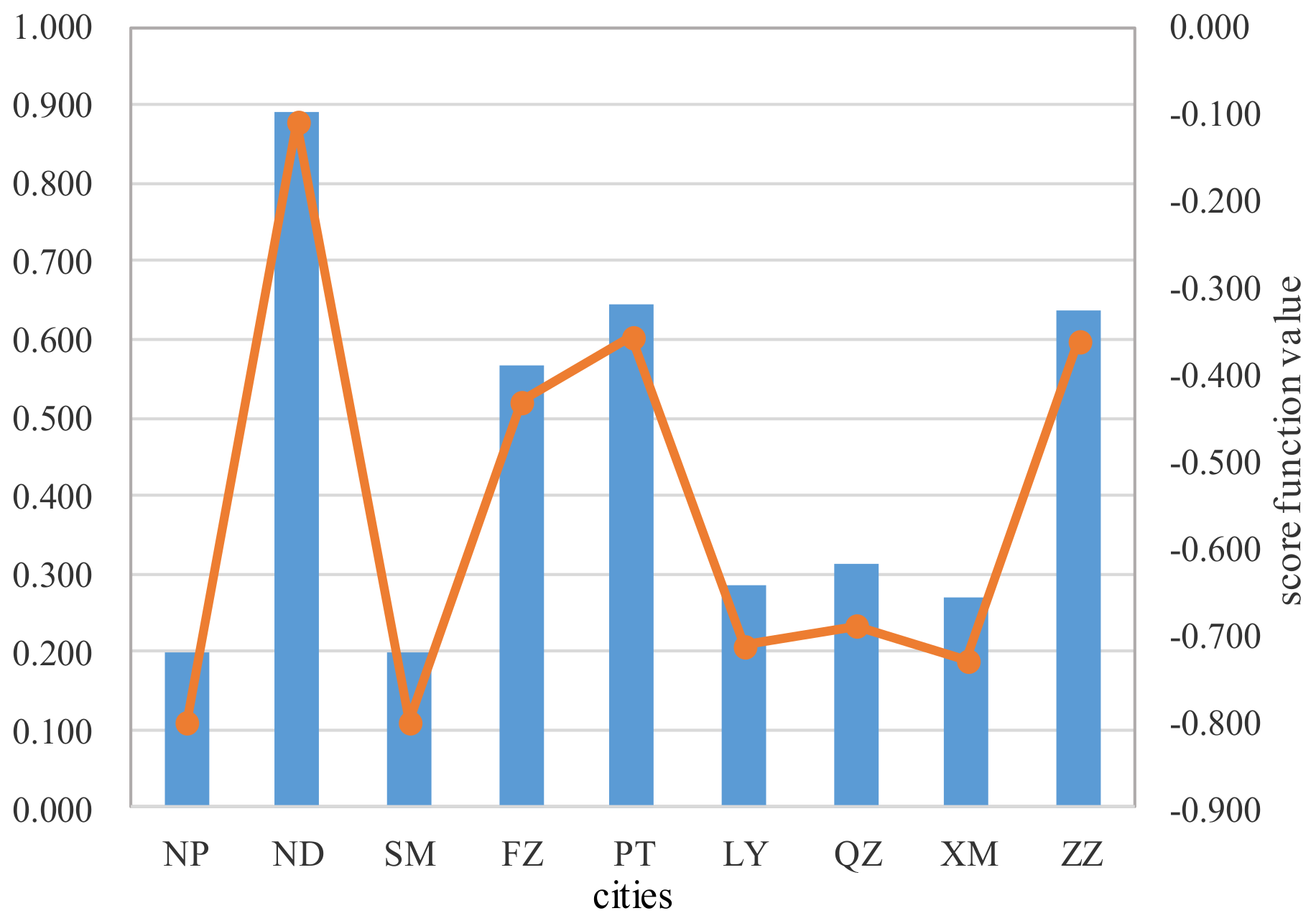
S ( d 1 N P ) = 0.801 , S ( d 2 N D ) = 0.109 , S ( d 3 S M ) = 0.801 , S ( d 4 F Z ) = 0.432 ,
S ( d 5 P T ) = 0.357 , S ( d 6 L Y ) = 0.714 , S ( d 7 Q Z ) = 0.690 , S ( d 8 X M ) = 0.730 ,
S ( d 9 Z Z ) = 0.360 .
Step 3
According to Definition 6, the ranking order of the nine cities is d 2 N D d 5 P T d 9 Z Z d 4 F Z d 7 Q Z d 6 L Y d 8 X M d 3 S M ~ d 1 N P . The ranking results of the cities are shown in Figure 1.
Step 4
End.

6.2. Comparative Analysis Based on Different Sorting Methods

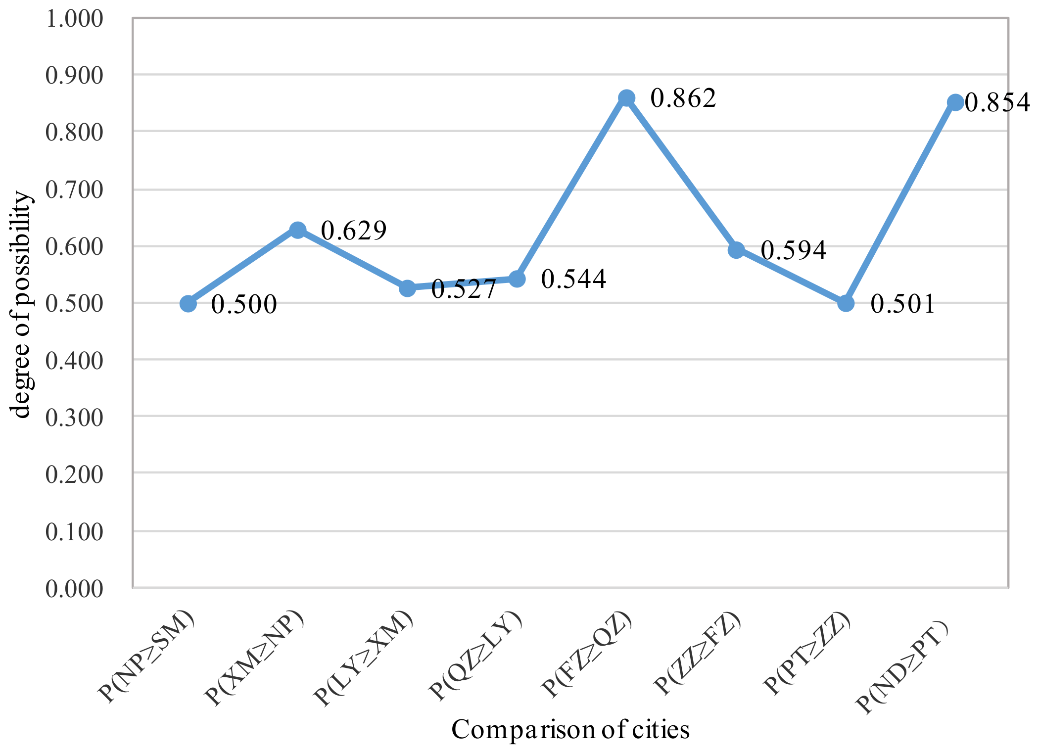
To illustrate the stability of the ranking results, the degree of possibility-based ranking method proposed in [33,45] is used in this paper. We obtain the matrix of degrees of possibility of the comprehensive assessment values of nine cities as follows:
P = N P N D S M F Z P T L Y Q Z X M Z Z     N P     N D     S M     F Z     P T     L Y     Q Z     X M     Z Z [ 0.500 0.000 0.500 0.000 0.000 0.344 0.302 0.371 0.000 1.000 0.500 1.000 0.944 0.854 1.000 1.000 1.000 0.843 0.500 0.000 0.500 0.000 0.000 0.344 0.302 0.371 0.000 1.000 0.056 1.000 0.500 0.402 0.913 0.862 0.943 0.406 1.000 0.146 1.000 0.598 0.500 1.000 0.980 1.000 0.501 0.656 0.000 0.656 0.087 0.000 0.500 0.456 0.527 0.000 0.698 0.000 0.698 0.138 0.020 0.544 0.500 0.570 0.038 0.629 0.000 0.629 0.057 0.000 0.473 0.430 0.500 0.000 1.000 0.157 1.000 0.594 0.499 1.000 0.962 0.100 0.500 ]
Here, N D P T Z Z F Z Q Z L Y X M S M ~ N P . The ranking order of the nine cities is also d 2 N D d 5 P T d 9 Z Z d 4 F Z d 7 Q Z d 6 L Y d 8 X M d 3 S M ~ d 1 N P . The ranking results of the cities are shown in Figure 2. As can be seen from the above results, the two sorting results are the same.

6.3. Comparative Analysis of Different Aggregation Operators

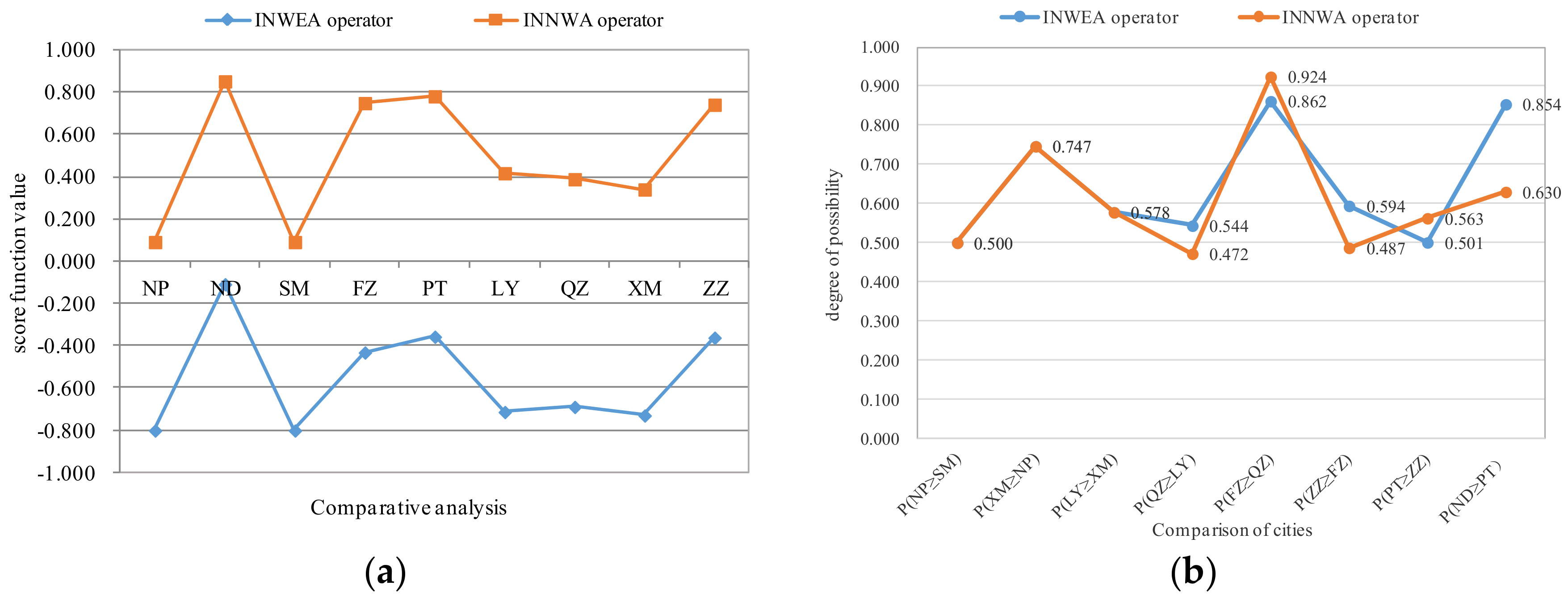
In order to illustrate the rationality and predominance of the proposed method, we compare this method with other methods [33]. The comparative analysis is shown in Table 2 and Figure 3.
First in Step 1, using the I N N W A operator proposed by [33] instead of the I N W E A operator to aggregate all evaluation information to obtain a comprehensive assessment value d i for each city, then using Definition 4 to calculate the score function value of d i as follows:
S ( d 1 N P ) = 0.092 ,   S ( d 2 N D ) = 0.853 ,   S ( d 3 S M ) = 0.092 ,   S ( d 4 F Z ) = 0.750 ,   S ( d 5 P T ) = 0.782 ,   S ( d 6 L Y ) = 0.418 , S ( d 7 Q Z ) = 0.389 ,   S ( d 8 X M ) = 0.340 ,   S ( d 9 Z Z ) = 0.742 .
Here, we compare and analyze several aggregation methods to illustrate the advantages of the proposed method.
(1) Can be seen from Table 2 and Figure 3, the two ranking results based on the I N W E A operator and the I N N W A operator are different. The main reason is that the positions and meanings of the attribute values and the attribute weights are different. For the I N W E A operator, its bases are positive real numbers and the exponents are interval neutrosophic numbers. It can deal with the decision making problem, in which attribute values are positive real numbers, and the attribute weights are interval neutrosophic numbers. However, the I N N W A operator is just the opposite. It needs to exchange the roles of the attribute values and the attribute weights because its bases are interval neutrosophic numbers and its exponents are positive real numbers. Therefore, it cannot be used to solve the typhoon disaster assessment problem in this paper, and the second ranking results in Table 2 and Figure 3 are unreasonable.
(2) Compared with the existing S V N W A A operator introduced in an SVNN environment [41], our method is a more generalized representation, and the S V N W A A operator is a special case. When the upper limit and lower limit of the INNs are the same, the I N W E A operator is equivalent to the S V N W E A operator.
(3) Compared with the existing I I F W E A operator of IIFNs [40] and the I F W E A operator of IFNs [39], our method uses interval neutrosophic weights, which include truth degree, falsity degree, and indeterminacy degree, and can deal with the indeterminate, incomplete, and inconsistent problems. However, the I I F W E A operator and I F W E A operator use intuitionistic fuzzy weights, which only contain truth degree and falsity degree, and cannot handle the assessment problem in this paper. Since IFN and IIFN are only special cases of interval NN, our exponential aggregation operator is the extension of the existing exponential operators [39,40,41].

7. Conclusions

In this paper, a typhoon disaster evaluation approach based on exponential aggregation operators of interval neutrosophic numbers under the neutrosophic fuzzy environment, is proposed. First, this paper introduced the exponential operational laws of INSs and INNs, which are a useful supplement to the existing neutrosophic fuzzy aggregation techniques. Then, we investigated a series of properties of these operational laws. Next, we discussed in detail some favorable properties of the interval neutrosophic weighted exponential aggregation (INWEA) operator.Finally, we applied the proposed decision making method successfully to the evaluation of typhoon disaster assessment. The research in this paper will be helpful to deepen the study of typhoon disaster evaluation and improve decision making for disaster reduction and disaster prevention. In addition, it provides methodological guidance for the handling of typhoon disasters and can improve the government’s ability to effectively improve disaster reduction. In future research, we will expand the proposed method and apply it to other natural disaster assessment problems. We will continue to study related theories of exponential aggregation operators in a neutrosophic fuzzy environment and their application in typhoon disaster assessment. The authors will also study the related theory of single-valued neutrosophic sets, interval-valued neutrosophic sets, bipolar neutrosophic sets, neutrosophic hesitant fuzzy sets, multi-valued neutrosophic sets, simplified neutrosophic linguistic sets, and their applications in typhoon disaster evaluation problems.

Author Contributions

All three authors contribute to this article, and the specific contribution is as follows: the idea and mathematical model were put forward by R.T., she also wrote the paper. W.Z. analyzed the existing work of the research problem and collected relevant data. Submission and review of the paper are the responsibility of S.C.

Funding

This research was funded by [Fujian Federation Of Social Science Circles] grant number [FJ2016C028], [The Education Department Of Fujian Province] grant numbers [JAT160556,JAT170113], [National Planning Office of Philosophy and Social Science] grant number [17CGL058], [Ministry of Education of the People's Republic of China] grant number [16YJC630008], [Fuzhou University] grant number [BPZD1601].

Acknowledgments

This research is supported by the Fujian Province Social Science Planning Project of China (No. FJ2016C028), Education and Scientific Research Projects of Young and Middle-aged Teachers of Fujian Province (No. JAT160556, JAT170113), Projects of the National Social Science Foundation of China (No. 17CGL058), Social Sciences Foundation of the Ministry of Education of China (No. 16YJC630008), and Fuzhou University Funding Project (No. BPZD1601).

Conflicts of Interest

The authors declare no conflicts of interest.

References

  1. Yu, D.J. Intuitionistic fuzzy theory based typhoon disaster evaluation in Zhejiang Province, China: A comparative Perspective. Nat. Hazards 2015, 75, 2559–2576. [Google Scholar] [CrossRef]
  2. Knutson, T.R.; Tuleya, R.E.; Kurihara, Y. Simulated increase of hurricane intensities in a CO2-warmed climate. Science 1998, 279, 1018–1020. [Google Scholar] [CrossRef] [PubMed]
  3. Zhang, Y.; Fan, G.F.; He, Y.; Cao, L.J. Risk assessment of typhoon disaster for the Yangtze River Delta of China. Geomat. Nat. Hazards Risk 2017, 8, 1580–1591. [Google Scholar] [CrossRef]
  4. Wang, G.; Chen, R.; Chen, J. Direct and indirect economic loss assessment of typhoon disasters based on EC and IO joint model. Nat. Hazards 2017, 87, 1751–1764. [Google Scholar] [CrossRef]
  5. Zhang, J.; Huang, H.; Che, X.; Zhang, M. Evaluation of Typhoon Disaster Losses of Hainan Island Rubber Plantation. In Proceedings of the 7th Annual Meeting of Risk Analysis Council of China Association for Disaster Prevention, Changsha, China, 4–6 November 2016; pp. 251–256. [Google Scholar]
  6. Lou, W.P.; Chen, H.Y.; Qiu, X.F.; Tang, Q.Y.; Zheng, F. Assessment of economic losses from tropical cyclone disasters based on PCA-BP. Nat. Hazards 2012, 60, 819–829. [Google Scholar] [CrossRef]
  7. Lu, C.L.; Chen, S.H. Multiple linear interdependent models (Mlim) applied to typhoon data from China. Theor. Appl. Climatol. 1998, 61, 143–149. [Google Scholar]
  8. Yang, A.; Sui, G.; Tang, D.; Lin, J.; Chen, H. An intelligent decision support system for typhoon disaster management. J. Comput. Inf. Syst. 2012, 8, 6705–6712. [Google Scholar]
  9. Li, C.; Zhang, L.; Zeng, S. Typhoon disaster evaluation based on extension of intuitionistic fuzzy TOPSIS method in Zhejiang Province of China. Int. J. Earth Sci. Eng. 2015, 8, 1031–1035. [Google Scholar]
  10. Ma, Q. A Fuzzy Synthetic Evaluation Model for Typhoon Disaster. Meteorol. Mon. 2008, 34, 20–25. (In Chinese) [Google Scholar]
  11. Chen, S.H.; Liu, X.Q. Typhoon disaster evaluation model based on discrete Hopfield neural network. J. Nat. Disasters 2011, 20, 47–52. [Google Scholar]
  12. He, X.R. Typhoon disaster assessment based on Dombi hesitant fuzzy information aggregation operators. Nat. Hazards 2018, 90, 1153–1175. [Google Scholar] [CrossRef]
  13. Smarandache, F. Neutrosophy: Neutrosophic Probability, Set, and Logic; American Research Press: Rehoboth, DE, USA, 1998. [Google Scholar]
  14. Smarandache, F. Neutrosophic set—A generalization of intuitionistic fuzzy set. IEEE Int. Conf. Granul. Comput. 2006, 1, 38–42. [Google Scholar]
  15. Zadeh, L.A. Fuzzy sets. Inf. Control 1965, 8, 338–353. [Google Scholar] [CrossRef] [Green Version]
  16. Atanassov, K.T. Intuitionistic fuzzy sets. Fuzzy Sets Syst. 1986, 20, 87–96. [Google Scholar] [CrossRef]
  17. Wang, H.B.; Smarandache, F.; Zhang, Y.Q. Single valued neutrosophic sets. Multisp. Multistruct. 2010, 4, 410–413. [Google Scholar]
  18. Ye, J. A multicriteria decision-making method using aggregation operators for simplified neutrosophic sets. Int. J. Fuzzy Syst. 2014, 26, 2459–2466. [Google Scholar]
  19. Wang, J.J.; Li, X.E. TODIM method with multi-valued neutrosophic sets. Control Decis. 2015, 30, 1139–1142. (In Chinese) [Google Scholar]
  20. Peng, J.J.; Wang, J.Q. Multi-valued Neutrosophic Sets and its Application in Multi-criteria Decision-making Problems. Neutrosophic Sets Syst. 2015, 10, 3–17. [Google Scholar] [CrossRef]
  21. Wang, H.; Smarandache, F.; Zhang, Y.Q.; Sunderraman, R. Interval Neutrosophic Sets and Logic: Theory and Applications in Computing; Hexis: Phoenix, AZ, USA, 2005. [Google Scholar]
  22. Zhang, H.Y.; Ji, P.J.; Wang, J.Q.; Chen, X.H. Improved Weighted Correlation Coefficient based on Integrated Weight for Interval Neutrosophic Sets and its Application in Multi-criteria Decision Making Problems. Int. J. Comput. Intell. Syst. 2015, 8, 1027–1043. [Google Scholar] [CrossRef]
  23. Ye, J. Multiple-attribute decision-making method under a single-valued neutrosophic hesitant fuzzy environment. J. Intell. Syst. 2014, 24, 23–36. [Google Scholar] [CrossRef]
  24. Tian, Z.P.; Wang, J.; Zhang, H.Y.; Chen, X.H.; Wang, J.Q. Simplified neutrosophic linguistic normalized weighted Bonferroni mean operator and its application to multi-criteria decision-making problems. Filomat 2015, 30, 3339–3360. [Google Scholar] [CrossRef]
  25. Biswas, P.; Pramanik, S.; Giri, B.C. Cosine Similarity Measure Based Multi-attribute Decision-making with Trapezoidal Fuzzy Neutrosophic Numbers. Neutrosophic Sets Syst. 2014, 8, 46–56. [Google Scholar]
  26. Ye, J. Trapezoidal neutrosophic set and its applicaion to multiple attribute decision-making. Neural Comput. Appl. 2015, 26, 1157–1166. [Google Scholar] [CrossRef]
  27. Deli, I. Interval-valued neutrosophic soft sets and its decision making. Int. J. Mach. Learn. Cybern. 2017, 8, 665–676. [Google Scholar] [CrossRef]
  28. Broumi, S.; Talea, M.; Bakali, A.; Smarandache, F. Single Valued Neutrosophic Graphs. J. New Theory 2016, 10, 86–101. [Google Scholar]
  29. Broumi, S.; Smarandache, F.; Talea, M.; Bakali, A. An Introduction to Bipolar Single Valued Neutrosophic Graph Theory. Appl. Mech. Mater. 2016, 841, 184–191. [Google Scholar] [CrossRef]
  30. Broumi, S.; Talea, M.; Bakali, A.; Smarandache, F. ON Strong Interval Valued Neutrosophic graphs. Crit. Rev. 2016, XII, 49–71. [Google Scholar]
  31. Liu, C.F.; Luo, Y.S. Correlated aggregation operators for simplified neutrosophic set and their application in multi-attribute group decision making. J. Intell. Fuzzy Syst. 2016, 30, 1755–1761. [Google Scholar] [CrossRef]
  32. Ye, J. Multiple attribute decision-making method based on the possibility degree ranking method and ordered weighted aggregation operators of interval neutrosophic numbers. J. Intell. Fuzzy Syst. 2015, 28, 1307–1317. [Google Scholar]
  33. Zhang, H.Y.; Wang, J.Q.; Chen, X.H. Interval neutrosophic sets and their application in multicriteria decision making problems. Sci. World J. 2014, 2014, 645653. [Google Scholar] [CrossRef] [PubMed]
  34. Liu, P.D.; Wang, Y.M. Multiple attribute decision-making method based on single-valued neutrosophic normalized weighted Bonferroni mean. Neural Comput. Appl. 2014, 25, 2001–2010. [Google Scholar] [CrossRef]
  35. Ye, J. Multiple attribute group decision making based on interval neutrosophic uncertain linguistic variables. Int. J. Mach. Learn. Cybern. 2017, 8, 837–848. [Google Scholar] [CrossRef]
  36. Peng, J.J.; Wang, J.Q.; Wu, X.H.; Wang, J.; Chen, X.H. Multi-valued Neutrosophic Sets and Power Aggregation Operators with Their Applications in Multi-criteria Group Decision-making Problems. Int. J. Comput. Intell. Syst. 2015, 8, 345–363. [Google Scholar] [CrossRef]
  37. Tan, R.; Zhang, W. Multiple attribute group decision making methods based on trapezoidal fuzzy neutrosophic numbers. J. Intell. Fuzzy Syst. 2017, 33, 2547–2564. [Google Scholar] [CrossRef]
  38. Şahin, R. Normal neutrosophic multiple attribute decision making based on generalized prioritized aggregation operators. Neural Comput. Appl. 2017, 1–21. [Google Scholar] [CrossRef]
  39. Gou, X.J.; Xu, Z.S.; Lei, Q. New operational laws and aggregation method of intuitionistic fuzzy information. J. Intell. Fuzzy Syst. 2016, 30, 129–141. [Google Scholar] [CrossRef]
  40. Gou, X.J.; Xu, Z.S.; Lei, Q. Exponential operations of interval-valued intuitionistic fuzzy numbers. Int. J. Mach. Learn. Cybern. 2016, 7, 501–518. [Google Scholar] [CrossRef]
  41. Lu, Z.; Ye, J. Exponential Operations and an Aggregation Method for Single-Valued Neutrosophic Numbers in Decision Making. Information 2017, 8, 62. [Google Scholar] [CrossRef]
  42. Şahin, R.; Liu, P. Some approaches to multi criteria decision making based on exponential operations of simplified neutrosophic numbers. J. Intell. Fuzzy Syst. 2017, 32, 2083–2099. [Google Scholar] [CrossRef]
  43. Ye, J. Exponential operations and aggregation operators of interval neutrosophic sets and their decision making methods. Springerplus 2016, 5–1488. [Google Scholar]
  44. Şahin, R. Multi-criteria neutrosophic decision making method based on score and accuracy functions under neutrosophic environment. Comput. Sci. 2014, 1–9. [Google Scholar] [CrossRef]
  45. Xu, Z. On method for uncertain multiple attribute decision making problems with uncertain multiplicative preference information on alternatives. Fuzzy Optim. Decis. Mak. 2005, 4, 131–139. [Google Scholar] [CrossRef]
Figure 1. Ranking results based on the score function.
Symmetry 10 00196 g001
Figure 2. Ranking results based on the degree of possibility.
Symmetry 10 00196 g002
Figure 3. Comparative analysis of different aggregation operators. (a) Ranking results of two operators based on the score function; (b) Ranking results of two operators based on the possibility degree.
Symmetry 10 00196 g003
Table 1. Decision matrix.
Attributesc1c2c3c4
Cities
Nanping (NP)0.20.20.20.2
Ningde (ND)0.90.80.70.4
Sanming (SM)0.20.20.20.2
Fuzhou (FZ)0.80.50.50.3
Putian (PT)0.70.70.60.3
Longyan (LY)0.40.30.30.2
Quanzhou (QZ)0.30.40.20.3
Xiamen (XM)0.30.30.30.2
Zhangzhou (ZZ)0.60.50.80.3
Table 2. Comparative analysis of different aggregation operators.
Different Aggregation MethodRanking Result
I N W E A operator of our method d 2 N D d 5 P T d 9 Z Z d 4 F Z d 7 Q Z d 6 L Y d 8 X M d 3 S M ~ d 1 N P
I N N W A operator of [33] d 2 N D d 5 P T d 4 F Z d 9 Z Z d 6 L Y d 7 Q Z d 8 X M d 3 S M ~ d 1 N P