Article

Predicting Ground Settlement Due to Symmetrical Tunneling through an Energy Conservation Method

Key Laboratory for Urban Underground Engineering of Ministry of Education, Beijing Jiaotong University, Beijing 100044, China
*
Author to whom correspondence should be addressed.
Symmetry 2018, 10(6), 186; https://doi.org/10.3390/sym10060186
Submission received: 27 April 2018 / Revised: 25 May 2018 / Accepted: 27 May 2018 / Published: 28 May 2018

Abstract

:
This paper presents an analytical method using the energy conservation principle to predict ground settlement due to symmetrically shaped tunnel construction in elastic ground conditions. Ground settlement is calculated by balancing the energy in shearing the soil, the work done by gravity, and the negative work done along the tunnel boundary. The proposed method was validated by finite-difference numerical simulations. According to the simulations, it was found that the direction of maximum shear stress under shear strain extension (SSE) was opposite to that under shear strain compression (SSC). The energy in shearing the soil can be obtained by using both the differential of ground displacement, and the fitted expression of maximum shear strain. Subsequently, ground deformation was predicted by the proposed method under three different conditions, and then compared with numerical results. Specific cases of ground settlement due to tunneling can be predicted by the proposed method, using the differential of the proposed empirical solutions. Ground settlements calculated by fitted expressions of maximum shear strain were closer to numerical results than those calculated by differentials. Deriving an empirical equation of maximum engineering shear strain from fitted expressions may be an innovative way for the proposed method to predict ground settlement.

1. Introduction

Tunnel constructions require the assessment of ground settlements as it is an essential aspect of the planning, design, and construction of tunneling projects in an urban environment. Ground deformation needs to be qualitatively estimated, and was previously described by various solutions. According to the empirical approach commonly used, Peck [1] calculated surface settlements using a Gaussian error function to describe the transverse surface settlement trough. The key parameter i, which denotes the lateral distance from the tunnel centerline to the point of inflection in the Gaussian distribution curve, was used to govern the width of the settlement trough. Subsequently, various researchers studied the correlations of the trough-width parameter i with tunnel diameter and tunnel overburden depth (O’Reilly and New [2], Clough and Schmidt [3]). As many tunnels are constructed in close vicinity to underground structures, it is also necessary to provide accurate predictions of both surface displacements, and subsurface displacements. Mair et al. [4] proposed a similar empirical method of obtaining both surface and subsurface displacements. Their proposed method was verified through centrifuge tests, and various field data from soft and stiff clays. Verruijt and Booker [5] estimated ground deformations by using isotropic, homogeneous elastic half-space equations, regarding the investigation proposed by Sagaseta [6]. A uniform, radial ground-deformation pattern and an original oval-shaped pattern were presented. Using the closed-form solution by Verruijt, Loganathan and Poulos [7] proposed a semi-empirical analytical method of calculating maximum surface settlement due to volume loss of shallow tunnels. However, the proposed solution described a wider surface-settlement trough when compared with field measurements. Bobet [8] also proposed an elastic solution which can be used for the preliminary design of shallow tunnels in saturated grounds.
Despite the fact that empirical approaches are useful for calculating ground settlements, they have various limitations. Numerical analyses provide a powerful tool to gain insight into the prediction of ground deformation in various circumstances. Many two-dimensional (2D) finite-element methods for modeling tunnel excavation were summarized by Potts and Zdravkovic [9], including the “gap” method, the “convergence confinement” method, the “progressive softening” method, and the “volume loss control” method. Three-dimensional (3D) numerical analyses can overcome the geometrical limitations of the two-dimensional plane-strain model. Although numerical methods are more effective and useful, Chou and Bobet [10,11] perceived that maximum surface settlement changed with an increase of the bottom boundary of models. The results calculated by numerical methods were related to the size of simulation models.
An innovative analytical method, named mobilizable strength design (MSD), was successfully implemented for shallow foundations (Osman and Bolton [12]), cantilever retaining walls (Osman and Bolton [13]), tunneling-induced ground settlements (Osman and Bolton [14]), and deep excavations. According to the principle of energy conservation, a kinematic mechanism is firstly required to characterize ground settlement due to tunneling. Subsequently, a representative stress–strain relationship is provided for soils participating in the mechanism. Finally, various kinds of energy can be calculated to estimate ground settlement. There are few related studies for the estimation of tunneling-induced ground settlements using energy conservation. In this paper, the new analytical method was assumed to behave elastically. This assumption was appropriate for rocks and stiff clays, in which ground settlements are small. Numerical analysis was first adopted to validate the proposed method. It was demonstrated that using energy conservation was a practical, innovative method of calculating ground settlements due to tunneling.

2. Energy Conservation Method for Tunneling-Induced Ground Deformation

The proposed method balanced the work and energy in pre-selected deformation mechanisms, so as to estimate ground settlements due to tunneling. In the case of tunneling without lines, the energy in shearing the soil, ΔE, must balance the work by gravity, ΔW, and the negative work along the tunnel boundary, ΔN. Thus, the energy-conservation equilibrium equation can be given by the following equation:
Δ E = Δ W Δ N ,
In terms of the displacement continuity, the energy in shearing the soil is calculated as follows:
Δ E = A r e a τ ε s d A r e a ,
where τ is the maximum shear stress, Area is the area of the mechanism we selected, and εs is the maximum engineering shear strain, which can be derived as follows:
ε s = ( ε x ε z ) 2 + γ x z 2 = ( δ u δ x δ v δ z ) 2 + ( δ u δ z + δ v δ x ) 2 ,
where εx is the strain in the horizontal direction (x-direction), εz is the strain in the vertical direction (z-direction), γxz is the shear strain in x-z plane, and u and v are the horizontal and vertical displacements of the ground.
The change in energy by gravity is simply given by the following equation:
Δ W = A r e a γ v d A r e a ,
where γ is the unit weight of the soil.
The negative work is mostly produced due to the decrease in initial force along the tunnel boundary. The initial force prevents the soil from deforming during the excavation of tunnels, and it can be resolved into horizontal and vertical components. Thus, the negative work can be obtained by the following equation:
Δ N = L i n e ( F x u + F z v ) d L i n e ,
where Line is the boundary of the tunnel, and Fx and Fz are the components of initial force in the horizontal and vertical directions along the tunnel boundary, respectively.
The finite-difference numerical method was used to validate the proposed method. All required energy was calculated by Equations (2), (4), and (5) in an effort to prove Equation (1) correct for the tunnel projects. Both volumetric strain and shear strain were also obtained, in an effort to illustrate that volumetric energy can be ignored under elastic-drainage conditions. Additionally, stress relief for tunneling is slightly different to that for excavating foundations. The direction of maximum shear stress changes above the crown, and below the invert of the tunnel.

3. Numerical Validation of Proposed Method

The numerical validation was done using by finite-difference-method FLAC3D 5.0 software [15] in the stress–strain plane, in which the radius of the tunnel was 3 m, and the overburden depths were 15 m, 20 m, and 25 m. The origin of the coordinates was the center of the tunnel. The horizontal boundary of the model ranged from 60 m to −60 m. The distance between the center of the tunnel and the bottom boundary of the model was 25 m. We assumed the elastic modulus of the soil to be 60 MPa. The Poisson’s ratio was 0.3, and the specific weight of the soil was 1900 kN/m3. The contours of the vertical displacements under various conditions are shown in Figure 1, in which the profiles of ground displacements were similar. ΔE was calculated from all zones of the models, and ΔW was calculated from all grid points. ΔN was only calculated from particular grid points along the tunnel boundary. All results for the three overburden depths are shown in Table 1.
Ground settlement occurs above the crown of the tunnel, and ground uplift occurs below the invert of the tunnel. The maximum settlements of the surface and the crown were 8.9 mm and 21.0 mm at a depth of 15 m, 9.9 mm and 28.9 mm at a depth of 20 m, and 10.6 mm and 36.8 mm at a depth of 25 m, respectively. The resultant errors were 10.6%, 3.7%, and 1.8% at the overburden depths of 15 m, 20 m, and 25 m, respectively. The deeper the tunnels were excavated, the smaller the errors were. In addition, the energy from shearing the soil under various conditions was larger than that due to gravity. The reason for this may be due to not keeping the volumetric strain as zero. In an effort to validate that the change of volumetric energy was very small, and that the resultant error was acceptable, we summed the volumetric strains of all zones and compared them with the maximum engineering shear strains. The compared results are shown in Table 2. The volumetric strains, εz + εx, were always unchanged when the stress plane transformed to the direction of maximum shear stress, and εy was always equal to zero.
The maximum engineering shear strains were several times as much as the volumetric strains. The change in volumetric energy was extremely small when compared with the energy in shearing the soil. The volumetric energy could be ignored without keeping the elasticity of the volumetric strain as zero. Therefore, it was feasible for the proposed method to calculate tunneling-induced ground settlements under elastic drained conditions because it satisfied the equilibrium equation of energy conservation.

4. Differences between Applications of the Method to Tunneling and to Excavating Foundations

When calculating the energy in shearing the soil using Equation (2), the stress relief due to tunneling should be analyzed. During the simulation, it was revealed that the maximum shear stresses of the zones within the blue areas increased in the negative direction, with an increase in maximum engineering shear strain. On the contrary, shear stresses within the red areas increased in the positive direction. The distinction depended on the direction of maximum shear stress, as shown in Figure 2. Hence, the behavior of the soil above the crown and below the invert was likely exhibiting shear strain extension (SSE), while the behavior of the soil on either side of the tunnel was likely exhibiting shear strain compression (SSC), as shown in Figure 2d. The shape and size of the SSE above the crown of the tunnel was similar and symmetrical along the centerline of the tunnel. The boundaries of the SSE around the crown were probably at x = 2.5 and z = 12.5 at a depth of 15 m, x = 2.5 and z = 17.5 at a depth of 20 m, and x = 2.5 and z = 22.5 at a depth of 25 m. The boundaries of the regions around the surface were at x = 10 at a depth of 15 m, x = 14 at a depth of 20 m, and x = 18 at a depth of 25 m. All slopes of the left and right boundary lines were approximately 1.5. On this account, the boundaries of these regions were assumed to be a straight line. Despite the fact that the calculation of shear energy under SSE conditions was the same as that under SSC conditions, the soil’s behavior due to tunneling should still be noted.

5. Prediction of Ground Deformation Using Proposed Method

Based on the analyses above, we perceived that the energy conservation method was able to estimate surface settlements. It was essential for this method to calculate the energy in shearing the soil. To obtain this energy, the expression for maximum engineering shear strain was required. However, when compared with the expression for surface settlements, the expression for maximum engineering shear strain is rarely researched. In this paper, two different approaches were used to calculate the shear strains and obtain the energy. The first approach obtained the energy indirectly through the differential of the vertical and horizontal displacements, as proposed by other researchers. The second approach obtained the energy directly through fitted expressions from the numerical results.

5.1. Prediction Using the Differential of Empirical Solutions

To obtain maximum shear strains using the differential, vertical and horizontal displacements of surface and subsurface were inevitably required. However, relatively few methods were available to estimate tunneling-induced subsurface settlements. Loganathan and Poulos [7] presented a closed-form solution for estimating subsurface settlements. Both vertical and horizontal displacements proposed by this method are given by the following equations:
v L = ε 0 R 2 ( z z 0 x 2 + ( z z 0 ) 2 + ( 3 4 μ ) z + z 0 x 2 + ( z + z 0 ) 2 2 z ( x 2 ( z + z 0 ) 2 ) ( x 2 + ( z + z 0 ) 2 ) ) exp ( ( 1.38 x 2 ( z 0 + R ) 2 + 0.69 z 2 z 0 2 ) ) ,
u L = ε 0 R 2 x ( 1 x 2 + ( z z 0 ) 2 + 3 4 μ x 2 + ( z + z 0 ) 2 4 z ( z + z 0 ) ( x 2 + ( z + z 0 ) 2 ) ) exp ( ( 1.38 x 2 ( z 0 + R ) 2 + 0.69 z 2 z 0 2 ) ) ,
where z0 is the tunnel depth as measured from the ground surface, ε0 is the ground loss, R is the radius of the tunnel, and vL and uL are the vertical and horizontal displacements.
Similarly, Mair et al. [4] also presented an empirical method to estimate subsurface settlements, which is given by the following equations:
v M = v max exp ( x 2 2 k 2 ( z 0 z ) 2 ) ,
v max = 1.25 ε 0 0.175 + 0.325 ( 1 z / z 0 ) R 2 z 0 ,
k = 0.175 + 0.325 ( 1 z / z 0 ) 1 z / z 0 ,
where vmax is the maximum subsurface settlement at depth z.
Following the work of Grant and Taylor [16], a distribution of horizontal displacement was proposed by the following equation:
u M = x H v M ,
where H is the distance between the plane of interest and the vector of interest for ground displacements. We assumed that H was equal to z0 so as to simplify this equation.
We obtained the differentials of the displacements using Equation (3). Both results of the calculations using the differentials had a similar distribution to that of the numerical maximum engineering shear strain. However, the peak values of the curves had some differences. The analytical curves of the differentials using both methods were illustrated for a depth of 20 m. All of the calculated results with a ground loss of 0.85% are shown in Figure 3.
Both these shear strain curves were wider than the numerical curves. For the same level of volume loss, Mair et al.’s [4] results decreased with depth, while Loganathan and Poulos’s [7] results increased with depth. The middle segments of the curves were concave near the top of the ground, when using Loganathan and Poulos’s results [7], and near the crown of the tunnel, when using Mair et al.’s results [4]. Notably, the middle segment of the surface curve using Loganathan and Poulos’s results [7] was convex, which was the same as that of the numerical surface curve.
In the proposed method, ε0 is the only unknown in the equations for ΔW and ΔE. The equation for ΔW is a linear term about ε0, while the equation for ΔE is a quadratic term about ε0. The unknown ε0 is equal to the expression for ΔE divided by that for ΔW. Consequently, ground displacements could be predicted once ground loss (ε0) was obtained. The maximum surface settlements were predicted in four different cases, including at depths of 15 m, 20 m, and 25 m. The results calculated using these two empirical methods were compared with the numerical results, and are shown in Table 3.
When compared with the numerical results (9.9 mm and 10.7 mm) at depths of 20 m and 25 m, the results using Mair et al.’s method [4] were 8.0 mm and 11.8 mm, respectively. We perceived that the results obtained using Mair et al.’s method [4] were suitable at depths ranging from 20 m to 25 m because the peak values of the curves within this range were close to those of the numerical curves. At depths of 15 m and 20 m, the results obtained using Mair et al.’s method [4] were slightly small. This was the reason for those shear strain curves being wider than the numerical curves. The resultant energy in shearing the soil was slightly large. The peak values near the crown were larger at shallower tunnel depths, and smaller when the tunnel was deeper. The calculated results were smaller at a depth of 15 m, and larger at a depth of 25 m.
The results calculated using Loganathan and Poulos’s method [7] were slightly small at a depth of 15 m, and considerably smaller when the tunnel was excavated deeper. This was due to the peak values of the shear strain curves increasing radically at depths below the crown of the tunnel. The denominators had a term of (z0z) in the expressions for vertical and horizontal displacement. When z was close to z0, the denominator was extremely small. Thus, the value of shear strain increased radically as the tunnel was excavated deeper. The energy in shearing the soil was extremely large. Accordingly, the obtained ground loss ε0 was fairly small. On the contrary, the energy in shearing the soil would not increase at shallower tunnel depths. We supposed this method was suitable for shallow tunnels.
The method using the differentials of horizontal and vertical soil displacements was inexact when calculating maximum surface settlements. This was probably due to the profiles of the vertical and horizontal soil displacements not fully conforming to the numerical curves. Additionally, horizontal soil displacement is not studied clearly. The errors using the differentials of horizontal and vertical displacements were beyond estimation. Despite this, the method using the differentials of vertical and horizontal displacements can still be used to calculate surface settlement under specific conditions.

5.2. Prediction Using Fitted Expressions of Numerical Results

The results of ground settlements and maximum shear strains were obtained and fitted by numerical analyses shown in Figure 4, Figure 5, Figure 6, Figure 7, Figure 8 and 
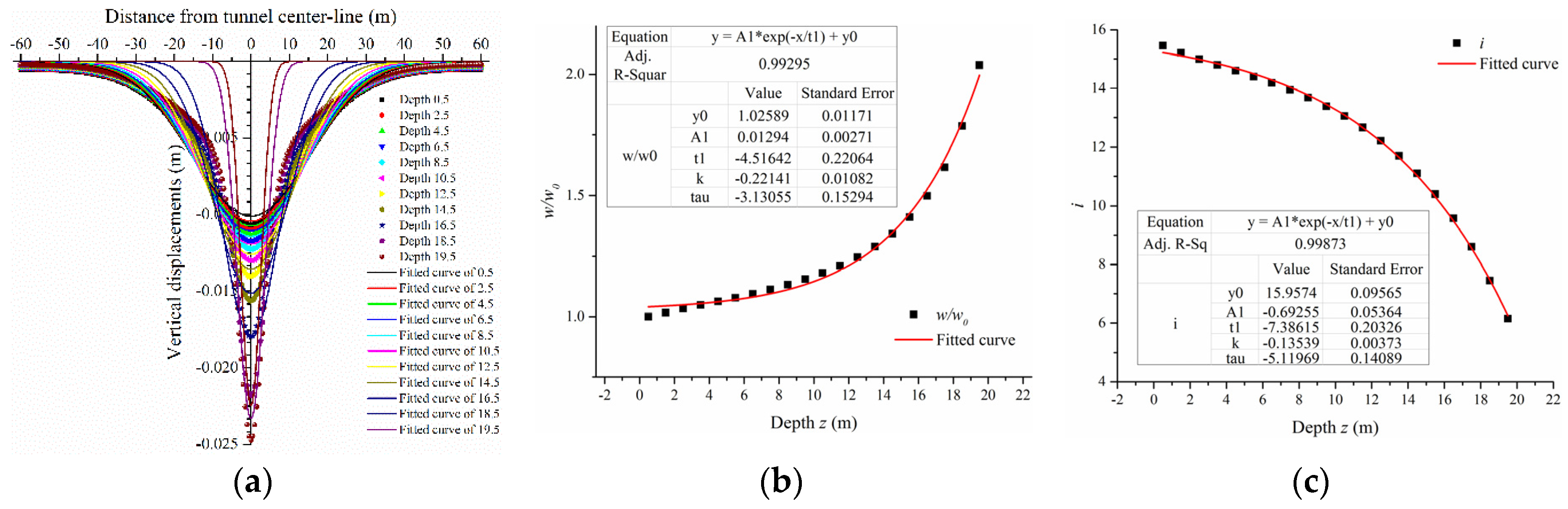
Figure 9. The vertical displacements satisfied a Gaussian distribution which was similar to Peck’s expression (Mair and Taylor [17]), and is given by the following equation:
v = w w 0 exp ( x 2 2 i s 2 ) ,
where w is the maximum displacement occurring at the tunnel centerline at depth z, is is the distance to the point of inflexion, and they are both satisfied by exponential functions at depth z. Note that w0 is the maximum surface settlement (x = 0, z = 0.5) which was later obtained. Accordingly, the fitted expressions were functions related to w0, x, and z.
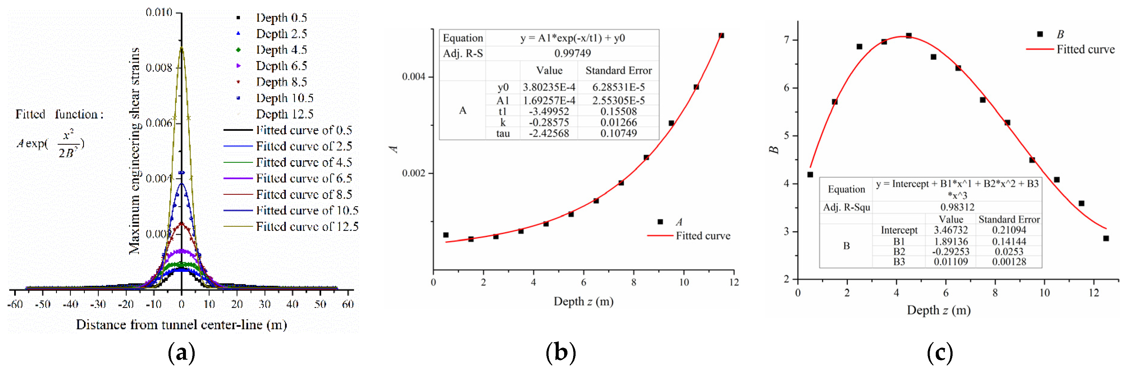
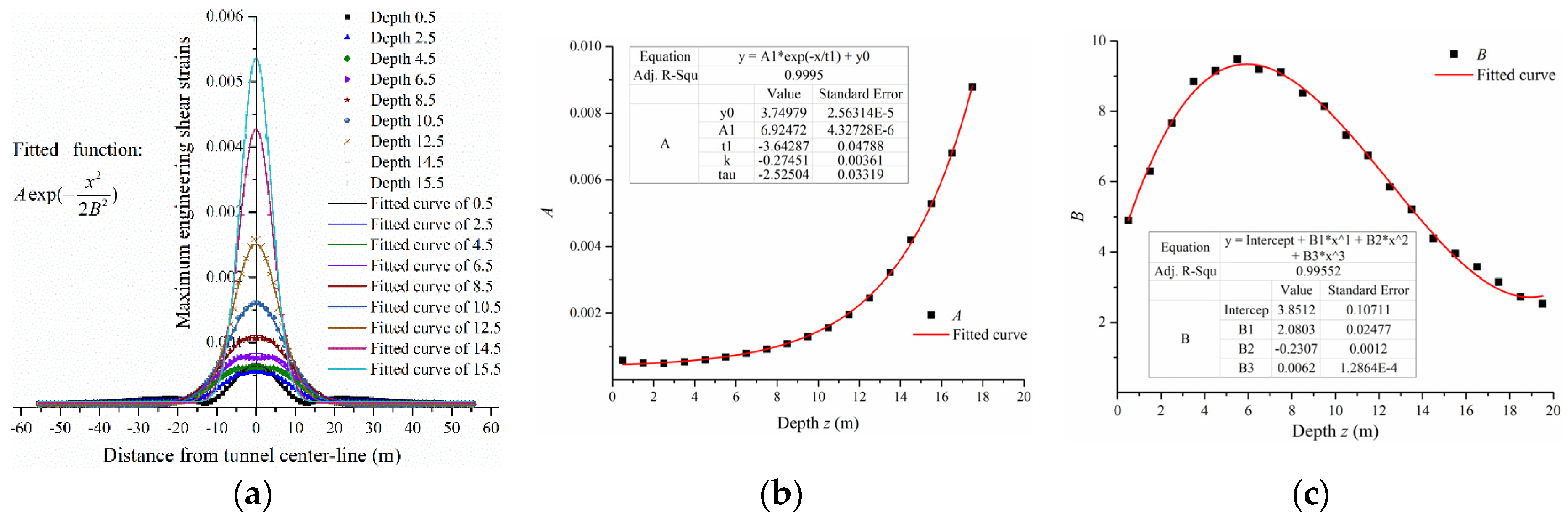
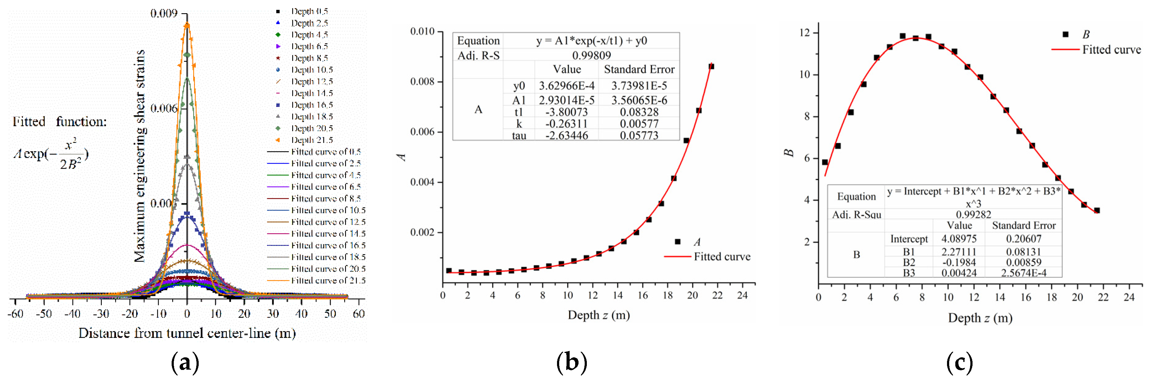
The predictions of maximum shear strains also satisfy a Gaussian distribution, as shown below.
ε s = A exp ( x 2 2 B 2 ) ,
where parameters A and B can be fitted by an exponential function and a cubic polynomial function, respectively. Note that the form of fitted functions resembles the Peck function because the maximum shear strain can be the differential of vertical and horizontal displacements. The forms of differential functions do not change due to the properties of differentials of exponential functions. Similarly, parameter A can also be fitted by an exponential function. The distance to the point of inflexion in the Peck function can be expanded by a polynomial function. Thus, it is suitable to fit parameter B using a cubic polynomial function. The expressions of all fitted parameters listed above are given in Appendix A. Note that some data below the crown of the tunnel were not shown, because there was either no data within the tunnel, or the data were extremely large.
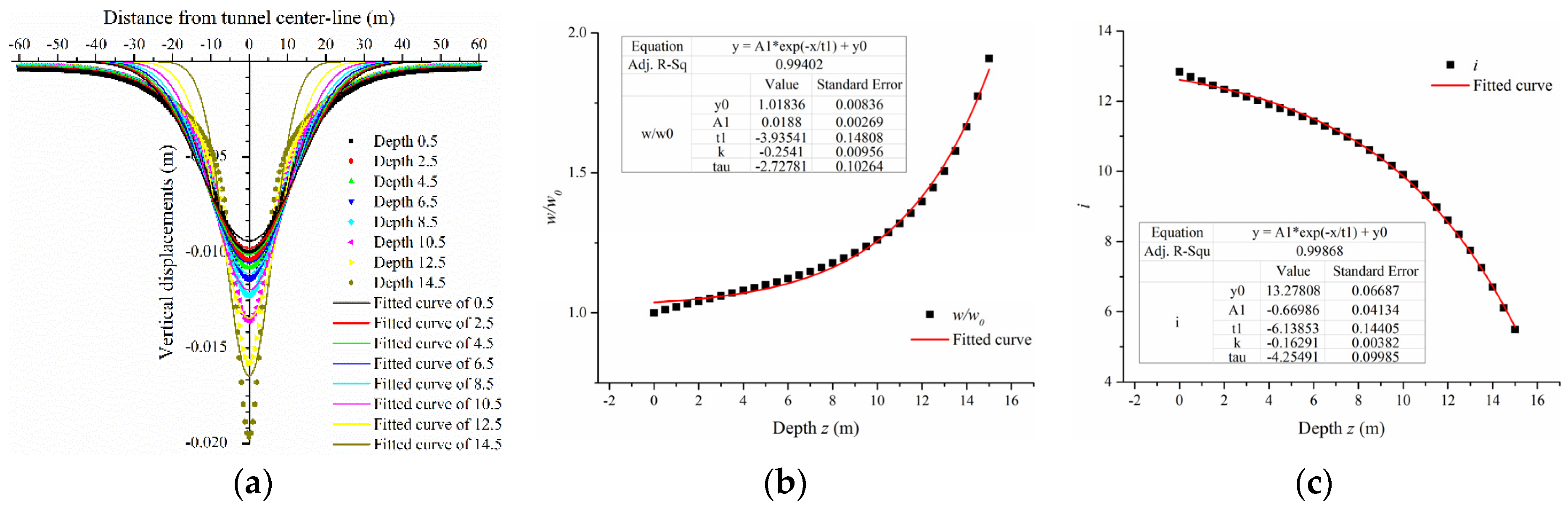
As shown in Figure 4, Figure 5 and Figure 6, the vertical displacements were not fitted perfectly. The reason was probably the distinction between the boundary of the numerical simulations and the Gaussian deformation mechanism. The total half-width of the surface settlement trough distributed in Gaussian was assumed to be 2.5 is (Mair et al. [4]). The soil outside the total width of the surface settlement trough was assumed to be stationary. However, the soil deformed at the same position in the numerical simulations even though the values were fairly small. Additionally, the deeper the buried soil was, the narrower the settlement trough became, and the larger the maximum vertical displacements were. This satisfied the conclusions presented by Fang et al. [18]. Therefore, the fitted expressions of vertical displacements were not exact at deeper depths. Most maximum values of the fitted expressions were smaller than those of the numerical results. Contrarily, the parameters w/w0 and is were both fitted exactly. The parameter w/w0 increased exponentially with an increase in depth z0, while the parameter is decreased exponentially.
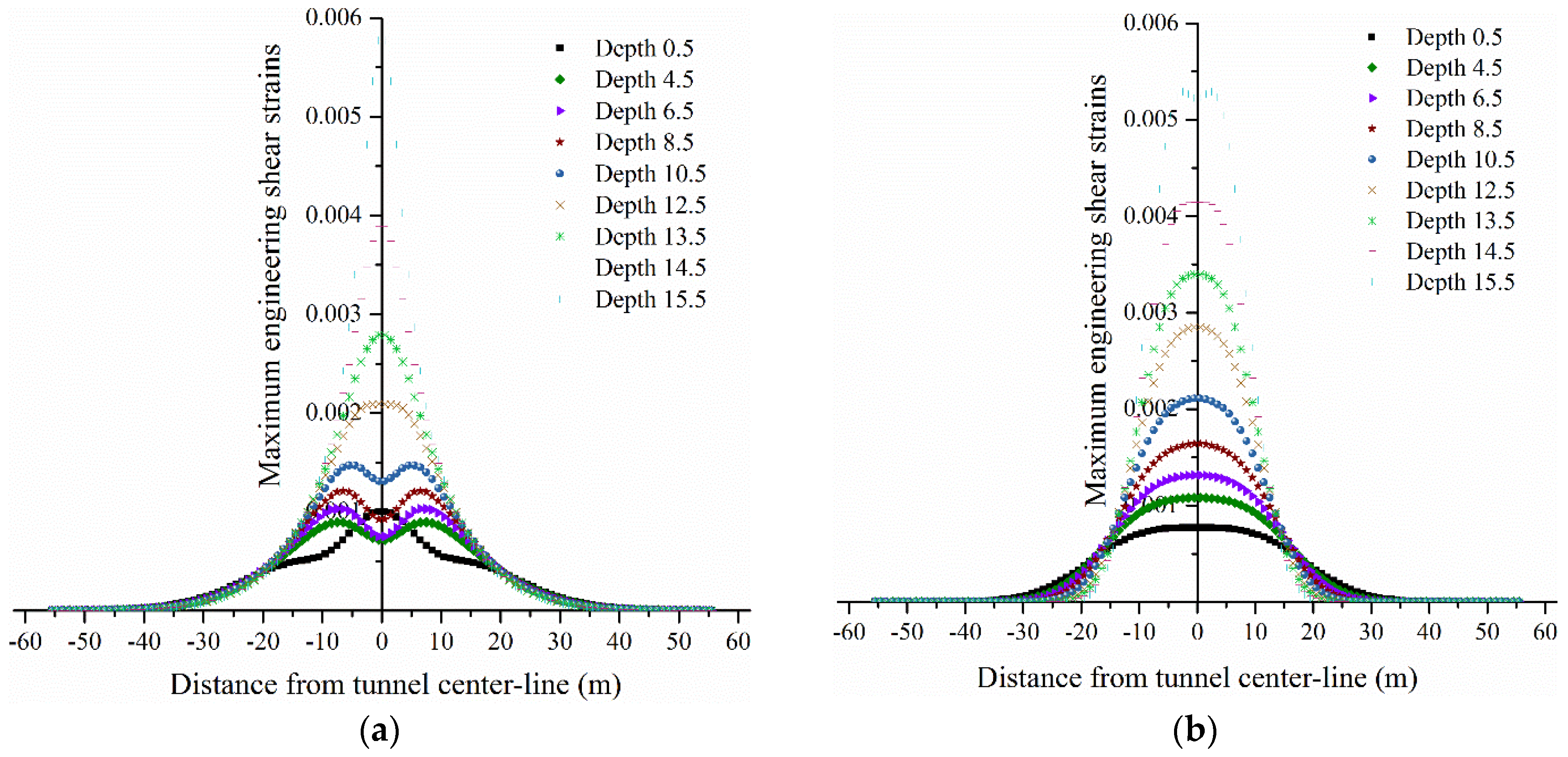
When compared with the vertical displacements, the maximum engineering shear strains were fitted perfectly. The coefficients of determinations of these fitted curves were larger than 0.99. The parameters A and B were also fitted exactly by the extracted results from the fitted expressions at each depth z. The parameter A decreased with an increase in depth z0. We perceived that the coefficients in the expressions changed regularly with overburden depth z0. Maximum engineering shear strain can probably be predicted by an accurate formula which has actual physical meaning. This formula is perhaps relative to the radius of the tunnel r and the overburden depth z0, and it can be studied further.
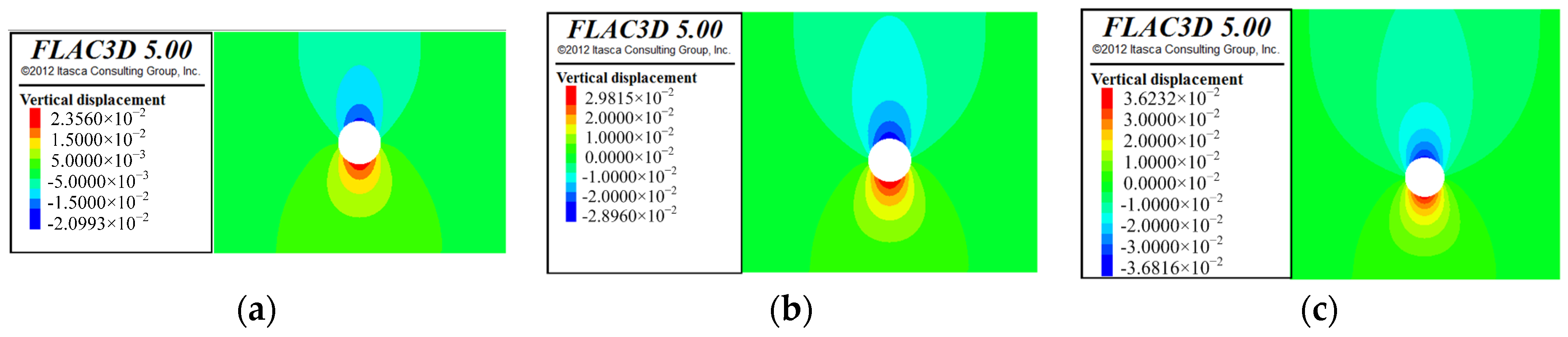
Based on the contours of vertical displacements in Figure 1, the ground displacements were separated into two different regions. The demarcation line was the location of the arch spring of tunnel. One region of displacement occurred in the upper area of the model, while the other occurred in the lower area of the model. As such, the upper area of the model was selected to calculate the settlement of the soil using Equation (1) and the fitted expressions above.
The mechanism was firstly divided into a series of unit elements (1 m × 1 m). Secondly, the energy of each element was calculated, and then summed to obtain ΔE and ΔW. According to the numerical analyses, the negative energy ΔN was about one-tenth of the total value of ΔW. ΔW − ΔN was modified by a coefficient of 1.2 due to the error between the vertical displacement results from the fitted expression and the numerical simulation. The reason for this treatment was that the vertical displacements from the fitted expressions were smaller than those in the numerical results, which was previously discussed. This was because ΔW − ΔN is a function about w0, and ΔE is a real number. Thus, all parameters were finally prepared for the calculation of w0. Using the Matlab software, the maximum surface settlements (w0) were calculated at depths of 15 m, 20 m and 25 m. All analytical results were compared with the numerical results, and are shown in Table 4.
The analytical results were 8.9 mm at a depth of 15 m, 10.3 mm at a depth of 20 m, and 11.1 mm at a depth of 25 mm. The maximum error between the calculation and the numerical results was 4.0 percent, and the minimum error was 3.5 percent. The method of calculating ground settlements due to tunneling using fitted expressions was better than that using the differentials of horizontal and vertical displacements. This research has improved the calculation of surface settlements by directly using fitted expressions of maximum engineering shear strains. The maximum engineering shear strains cannot yet be predicted by the arbitrary location of the tunnel z0, and the tunnel diameter r. The fitted expressions are worth studying further so as to calculate the surface and subsurface settlements.

6. Conclusions

This paper predicted ground settlements due to tunneling in a simple plane-strain displacement mechanism. The soil was assumed to be isotropic, homogeneous elastic material. The maximum surface settlements were calculated from an equilibrium equation, by balancing the work done by gravity against the energy in shearing the soil and the negative work done obstructing the soil’s deformation around the tunnel. To obtain these various kinds of energy, two methods were used to predict the vertical displacements and maximum engineering shear strains. One was obtained indirectly using the differentials of vertical and horizontal displacements which were proposed by other researchers. The other was obtained directly using the fitted expressions from the numerical results. Both analytical results were compared with the numerical results. The key conclusions obtained were as follows:
(1) The proposed method using energy conservation was validated by finite-difference-element numerical simulations of various cases. The volumetric energy could be ignored without keeping the volumetric strain as zero under elastic conditions.
(2) When compared with some foundation projects, SSE regions due to tunneling existed above the crown and below the invert of the tunnel. These regions had similar profiles which were related to overburden depths. It was significant to obtain the energy in shearing the soil before calculating the maximum surface settlement.
(3) The surface and subsurface settlements could be predicted by the proposed method using either empirical or closed-form solutions, as long as a suitable deformation mechanism was given. To obtain the shear strain in an effort to calculate the energy in shearing, the differentials of vertical and horizontal displacements could also be used. However, the accuracy of this method depended on the given deformation mechanism.
(4) The numerical results of the vertical displacements and maximum engineering shear strains could be fitted by simplified Gaussian distributions, and the parameters in these expressions were fitted by simple exponential and cubic polynomial functions. It was shown that all parameters perhaps had some rules regarding the location and radius of the tunnel, which is essential to study further.
(5) Directly calculating surface settlement using fitted maximum engineering shear strains was a creative method. The analytical results of maximum surface settlement were in great agreement with the numerical results. The error of this method was less than 5%. The proposed method of calculating surface settlement using fitted expressions was better than the method using differentials.

Author Contributions

The authors contributed equally to this work.

Acknowledgments

The authors gratefully acknowledge the financial support by the Fundamental Research Funds for the Central Universities under Grant 2016JBZ009, and the Chinese National Natural Science Foundation under Grant 51678035.

Conflicts of Interest

The authors declare no conflict of interest.

Appendix A

The fitted parameters of vertical settlements under various conditions.
w w 0 = 0.04283 exp ( z 3.77468 ) + 0.96471 .
i s = 0.55415 exp ( z 4.83016 ) + 9.40984 . ( depth   15   m )
w w 0 = 0.0188 exp ( z 3.9354 ) + 1.01836 .
i s = 0.66986 exp ( z 6.13853 ) + 13.27808 . ( depth   20   m )
w w 0 = 0.01294 exp ( z 4.51642 ) + 1.02589 .
i s = 0.69255 exp ( z 7.38615 ) + 15.95741 . ( depth   25   m )
The fitted parameters of maximum engineering shear strains under various conditions.
A = 1.69257 × 10 4 exp ( z 3.49952 ) + 3.80235 × 10 4 .
B = 3.4673 + 1.8913 z 0.2925 z 2 + 0.011 z 3 . ( depth   15   m )
A = 6.92472 × 10 5 exp ( z 3.64287 ) + 3.74979 × 10 4 .
B = 3.85123 + 2.08032 z 0.2307 z 2 + 0.00622 z 3 . ( depth   20   m )
A = 2.93014 × 10 5 exp ( z 3.80073 ) + 3.62966 × 10 4 .
B = 4.0897 + 2.2711 z 0.198 z 2 + 0.0042 z 3 . ( depth   25   m )

References

  1. Peck, R.B. Deep excavation and tunnelling in soft ground. In Proceedings of the 7th International Conference on Soil Mechanics and Foundation Engineering, Mexico City, Mexico, 25–29 August 1969; Sociedad Mexicana de Mecanica: Mexico City, Mexico, 1969; Volume 3, pp. 225–290. [Google Scholar]
  2. O’Reilly, M.P.; New, B.M. Settlements above tunnels in the United Kingdom—Their magnitude and prediction. In Tunnelling ’82, 3rd ed.; Institute of Mining and Metallurgy: London, UK, 1982; pp. 173–181. ISBN 090048862X. [Google Scholar]
  3. Clough, G.W.; Schmidt, B. Design and performance of excavations and tunnels in soft clay. In Soft Clay Engineering; Brand, E.W., Brenner, R.P., Eds.; Elsevier: Amsterdam, The Netherlands, 1981; pp. 569–634. ISBN 9780444417848. [Google Scholar]
  4. Mair, R.J.; Taylor, R.N.; Bracegirdle, A. Subsurface settlement profiles above tunnels in clays. Géotechnique 1993, 43, 315–320. [Google Scholar] [CrossRef]
  5. Verruijt, A.; Booker, J.R. Surface settlements due to deformation of a tunnel in an elastic half plane. Géotechnique 1996, 46, 753–756. [Google Scholar] [CrossRef]
  6. Sagaseta, C. Analysis of undrained soil deformation due to ground loss. Géotechnique 1987, 37, 301–320. [Google Scholar] [CrossRef]
  7. Loganathan, N.; Poulos, H.G. Analytical prediction of tunneling-induced ground movements in clays. ASCE J. Geotech. Geoenviron. Eng. 1998, 124, 846–856. [Google Scholar] [CrossRef]
  8. Bobet, A. Analytical solutions of shallow tunnels in saturated ground. ASCE J. Eng. Mech. 2001, 127, 1258–1266. [Google Scholar] [CrossRef]
  9. Potts, D.M.; Zdravkovic, L.; Zdravković, L. Finite Element Analysis in Geotechnical Engineering: Application; Thomas Telford: London, UK, 2001; ISBN 9780727727831. [Google Scholar]
  10. Chou, W.; Bobet, A. Response by the authors to Verruijt, A.; Sagaseta, C.; Strack, O.E. Discussion to the paper: Chou, W.; Bobet, A. Prediction s of ground deformations in shallow tunnels in clay. Tunn. Undergr. Space Technol. 2003, 18, 95–97. [Google Scholar] [CrossRef]
  11. Chou, W.; Bobet, A. Prediction s of ground deformations in shallow tunnels in clay. Tunn. Undergr. Space Technol. 2002, 17, 3–19. [Google Scholar] [CrossRef]
  12. Osman, A.S.; Bolton, M.D. Simple plasticity- based prediction of the undrained settlement of shallow circular foundations on clay. Géotechnique 2005, 55, 435–447. [Google Scholar] [CrossRef] [Green Version]
  13. Osman, A.S.; Bolton, M.D. A new design method for retaining walls in clay. Can. Geotech. J. 2004, 41, 451–466. [Google Scholar] [CrossRef]
  14. Osman, A.S.; Bolton, M.D.; Mair, R.J. Predicting 2D ground movements around tunnels in undrained clay. Géotechnique 2006, 56, 597–604. [Google Scholar] [CrossRef] [Green Version]
  15. Itasca Consulting Group, Inc. FLAC3D—Fast Lagrangian Analysis of Continua in 3 Dimensions, Version 5.0; Itasca: Minneapolis, MN, USA, 2012. [Google Scholar]
  16. Grant, R.J.; Taylor, R.N. Tunnelling-induced ground movements in clay. Proc. Inst. Civ. Eng. Geotech. Eng. 2000, 143, 43–55. [Google Scholar] [CrossRef]
  17. Mair, R.J.; Taylor, R.N. Bored tunneling in urban environment. In Proceedings of the 14th International Conference on Soil Mechanics and Foundation Engineering, Hamburg, Germany, 6–12 September 1997; Volume 4, pp. 2353–2385. [Google Scholar]
  18. Fang, Y.S.; Wu, C.T.; Chen, S.F.; Liu, C. An estimation of subsurface settlement due to shield tunneling. Tunn. Undergr. Space Technol. 2014, 44, 121–129. [Google Scholar] [CrossRef]
Figure 1. Vertical displacements under various conditions: (a) overburden depth of 15 m, (b) overburden depth of 20 mn (c) and overburden depth of 25 m.
Symmetry 10 00186 g001
Figure 2. Behavior of soil due to tunneling under various conditions: (a) overburden depth of 15 m, (b) overburden depth of 20 m, (c) and overburden depth of 25 m. (d) Direction of maximum shear stress.
Symmetry 10 00186 g002
Figure 3. Calculated maximum engineering shear strains at a depth of 20 m: (a) maximum engineering shear strains using the differential of Loganathan and Poulos’s [7] formulas, (b) and maximum engineering shear strains using the differential of Mair et al.’s [4] formulas.
Symmetry 10 00186 g003
Figure 4. (a) Vertical displacements and fitted curves at various depths up to 15 m. (b) Parameter w/w0 and its fitted curve at various depths. (c) Parameter is and its fitted curve at various depths.
Symmetry 10 00186 g004
Figure 5. (a) Vertical displacements and fitted curves at various depths up to 20 m. (b) Parameter w/w0 and its fitted curve at various depths. (c) Parameter is and its fitted curve at various depths.
Symmetry 10 00186 g005
Figure 6. (a) Vertical displacements and fitted curves at various depths up to 25 m. (b) Parameter w/w0 and its fitted curve at various depths. (c) Parameter is and its fitted curve at various depths.
Symmetry 10 00186 g006
Figure 7. (a) Maximum engineering shear strains and fitted curves at various depths up to 15 m. (b) Parameter A and its fitted curve at various depths. (c) Parameter B and its fitted curve at various depths.
Symmetry 10 00186 g007
Figure 8. (a) Maximum engineering shear strains and fitted curves at various depths up to 20 m. (b) Parameter A and its fitted curve at various depths. (c) Parameter B and its fitted curve at various depths.
Symmetry 10 00186 g008
Figure 9. (a) Maximum engineering shear strains and fitted curves at various depths up to 25 m. (b) Parameter A and its fitted curve at various depths. (c) Parameter B and its fitted curve at various depths.
Symmetry 10 00186 g009
Table 1. Calculation results of the three models.
Maximum Settlement of Surface (mm)Maximum Settlement of Crown (mm)ΔE (kN·m)ΔW (kN·m)ΔN (kN·m)Δ (kN·m)Error (%)
Depth 15 m8.921.0187.3199.932.419.810.6
Depth 20 m9.928.9415.6456.856.615.43.7
Depth 25 m10.636.8677.6753.287.912.31.8
Note that Δ = ΔE − (ΔW − ΔN), and the error is equal to Δ divided by ΔE.
Table 2. Volumetric strains and shear strains in the numerical models.
Shear StrainsVolume StrainsThe Ratio (%)
Depth 15 m4.5540.1112.443
Depth 20 m6.531−0.0790.121
Depth 25 m8.620−0.0360.419
Table 3. Prediction of maximum surface settlement using Mair et al.’s [4] and Loganathan & Poulos’s [7] methods.
Numerical Method (mm)Mair et al.’s [4] Method (mm)Loganathan and Poulos’s [7] Method (mm)
Depth 15 m8.65.18.2
Depth 20 m9.98.05.0
Depth 25 m10.711.83.3
Table 4. Analytical maximum surface settlements (w0) compared with numerical results.
Numerical Result (mm)Analytical Result (mm)Error (%)
Depth 15 m8.68.93.5
Depth 20 m9.910.34.0
Depth 25 m10.711.13.7

