PFS: Particle-Filter-Based Superpixel Segmentation

Abstract
:1. Introduction
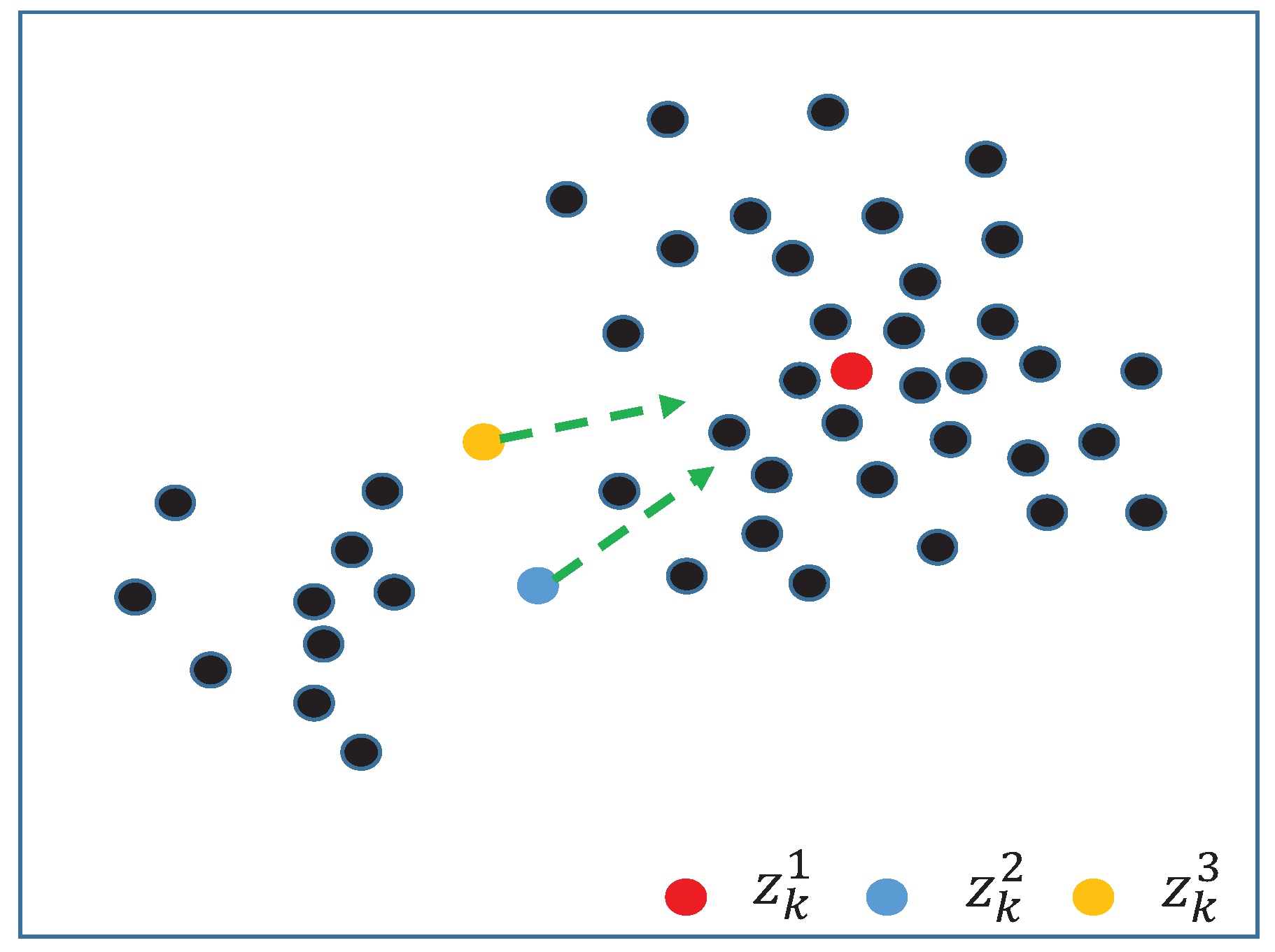
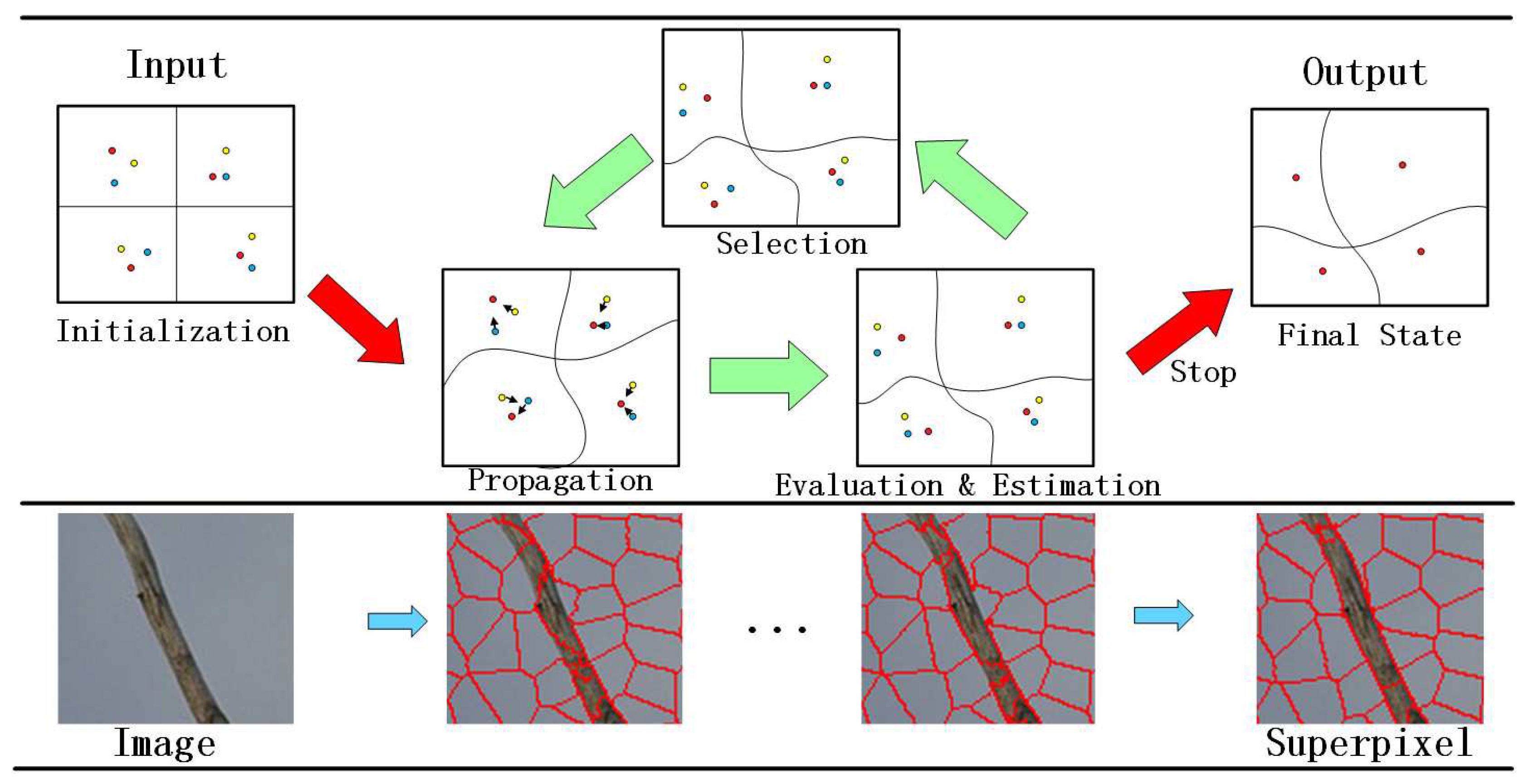
- We propose a novel superpixel segmentation method based on the particle filter, which extends the original tracking problem to region clustering. Multiple particles are used to approximate superpixel centers, which could highly dispersedly be located in feature space to generate a much lower intra-cluster distance.
- Moving and perturbing processes are introduced to guide the propagation step of those particles, which reformulates the particle filter to fit our region cluster problem.
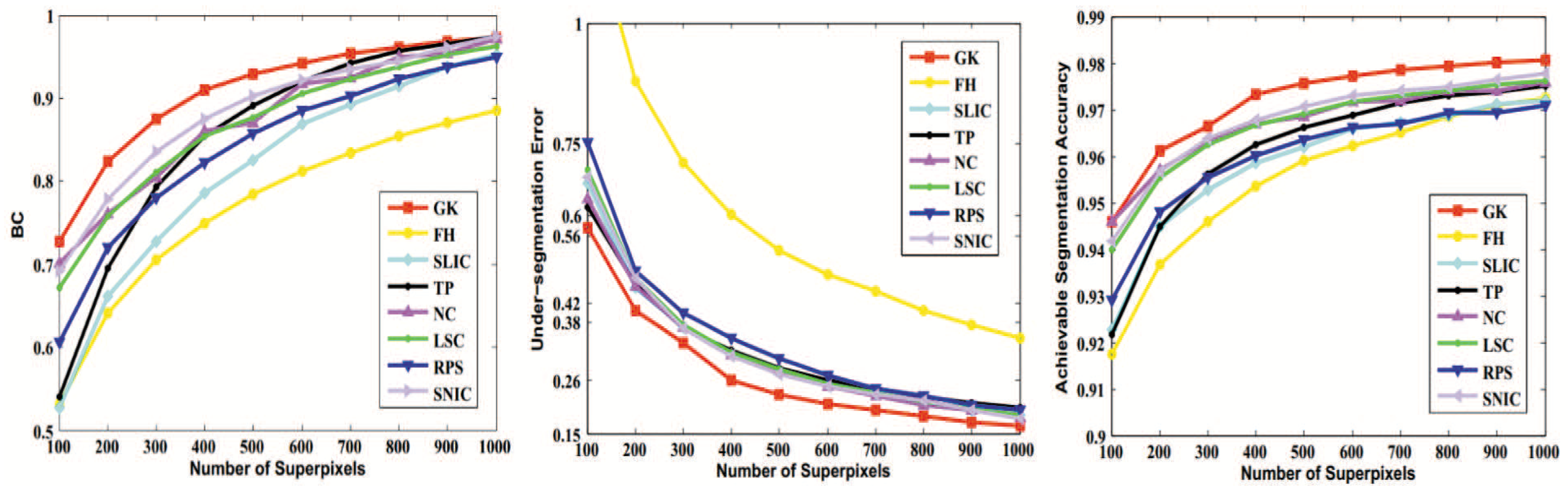
- The segmentation performance of PFS outperforms seven state-of-the-art methods on a quantitative benchmark.
2. Related Work
3. Particle Filtering
4. Superpixel Segmentation via Particle Filtering
4.1. Problem Formulation
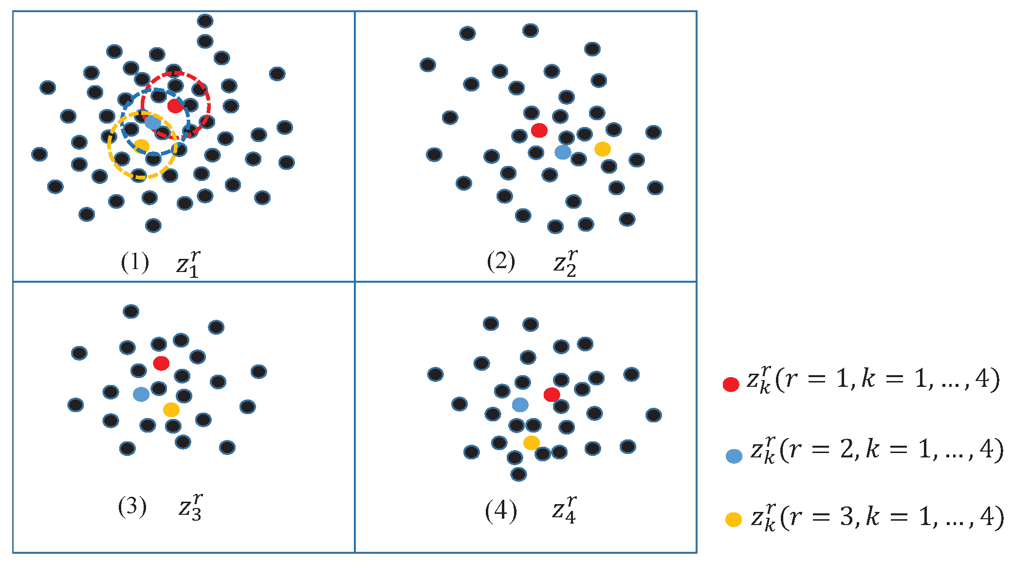
4.2. Initial Particles’ Selection
4.3. Propagation
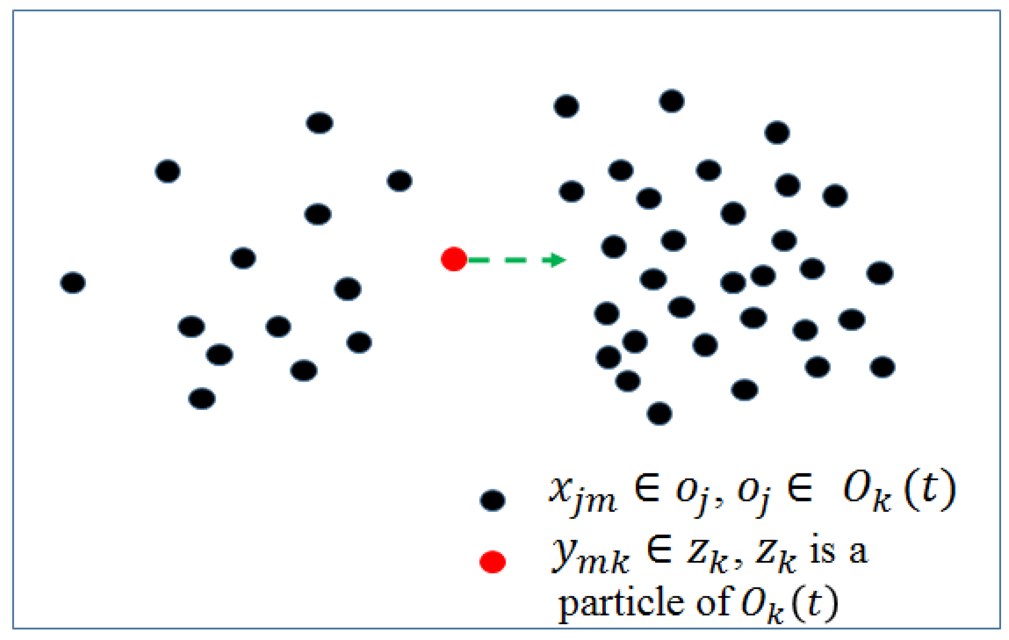
4.3.1. Movement
4.3.2. Perturbation
4.4. Evaluation and Estimation
| Algorithm 1 Algorithm for PFS. |
Require:
|
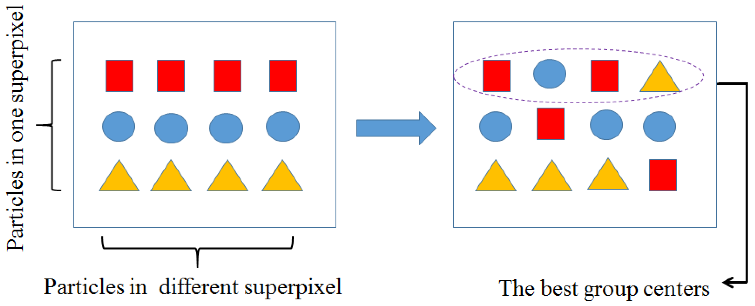
4.5. Selection
5. Experiment
5.1. Performance Evaluation
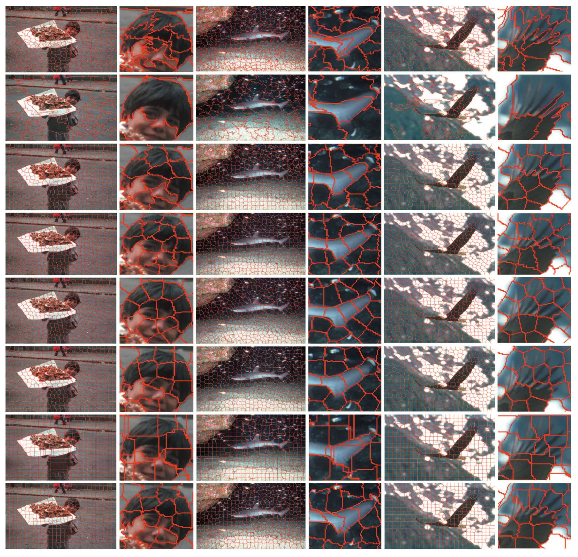
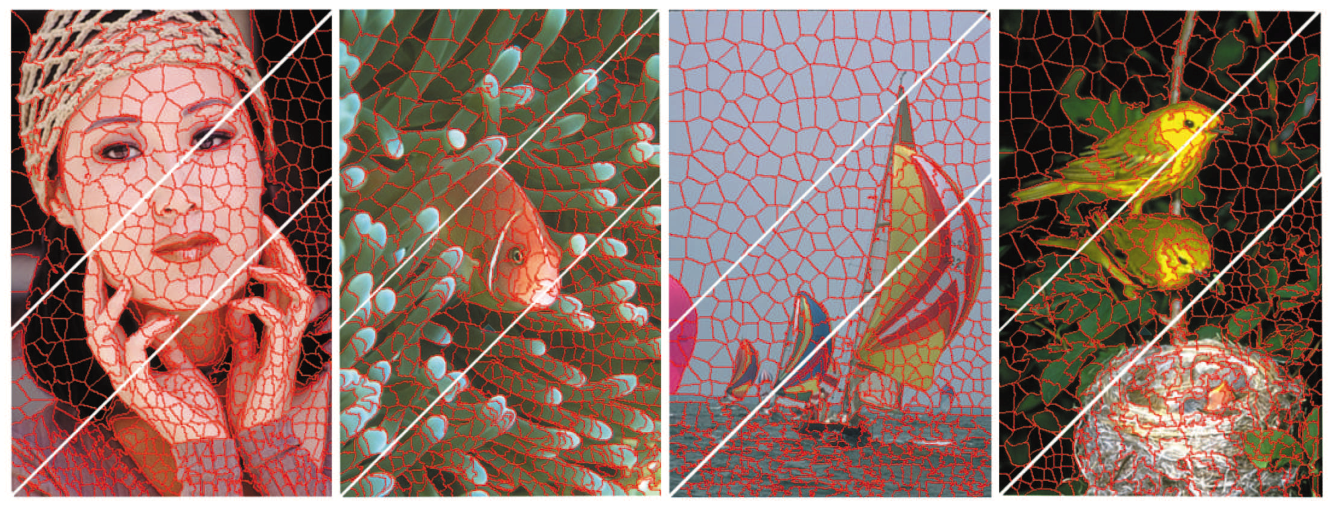
5.2. Visual Comparison
6. Conclusions
Author Contributions
Acknowledgments
Conflicts of Interest
References
- Han, B.J.; Sim, J.Y. Saliency Detection for Panoramic Landscape Images of Outdoor Scenes. J. Vis. Commun. Image Represent. 2017. [Google Scholar] [CrossRef]
- Xiao, Y.; Wang, L.; Jiang, B.; Tu, Z.; Tang, J. A global and local consistent ranking model for image saliency computation. J. Vis. Commun. Image Represent. 2017, 46, 199–207. [Google Scholar] [CrossRef]
- Fareed, M.M.S.; Ahmed, G.; Chun, Q. Salient region detection through sparse reconstruction and graph-based ranking. J. Vis. Commun. Image Represent. 2015, 32, 144–155. [Google Scholar] [CrossRef]
- Zhu, H.; Meng, F.; Cai, J.; Lu, S. Beyond pixels: A comprehensive survey from bottom-up to semantic image segmentation and cosegmentation. J. Vis. Commun. Image Represent. 2016, 34, 12–27. [Google Scholar] [CrossRef]
- Fulkerson, B.; Vedaldi, A.; Soatto, S. Class segmentation and object localization with superpixel neighborhoods. In Proceedings of the 2009 IEEE 12th International Conference on Computer Vision, Kyoto, Japan, 29 September–2 October 2009; pp. 670–677. [Google Scholar]
- Luo, B.; Li, H.; Song, T.; Huang, C. Object segmentation from long video sequences. In Proceedings of the 23rd ACM International Conference on Multimedia, Brisbane, Australia, 26–30 October 2015; pp. 1187–1190. [Google Scholar]
- Uijlings, J.R.; Van De Sande, K.E.; Gevers, T.; Smeulders, A.W. Selective search for object recognition. Int. J. Comput. Vis. 2013, 104, 154–171. [Google Scholar] [CrossRef]
- Mori, G.; Ren, X.; Efros, A.A.; Malik, J. Recovering human body configurations: Combining segmentation and recognition. In Proceedings of the 2004 IEEE Computer Society Conference on Computer Vision and Pattern Recognition, Washington, DC, USA, 27 June–2 July 2004; Volume 2, pp. II-326–II-333. [Google Scholar]
- Yuan, Y.; Fang, J.; Wang, Q. Robust Superpixel Tracking via Depth Fusion. IEEE Trans. Circuits Syst. Video Technol. 2014, 24, 15–26. [Google Scholar] [CrossRef]
- Shi, J.; Malik, J. Normalized cuts and image segmentation. IEEE Trans. Pattern Anal. Mach. Intell. 2000, 22, 888–905. [Google Scholar]
- Felzenszwalb, P.F.; Huttenlocher, D.P. Efficient Graph-Based Image Segmentation. Int. J. Comput. Vis. 2004, 59, 167–181. [Google Scholar] [CrossRef]
- Moore, A.P.; Prince, S.J.D.; Warrell, J.; Mohammed, U.; Jones, G. Superpixel lattices. In Proceedings of the 2008 IEEE Conference on Computer Vision and Pattern Recognition, Anchorage, AK, USA, 23–28 June 2008; pp. 1–8. [Google Scholar]
- Moore, A.P.; Prince, S.J.; Warrell, J. Lattice Cut—Constructing superpixels using layer constraints. In Proceedings of the 2010 IEEE Conference on Computer Vision and Pattern Recognition (CVPR), San Francisco, CA, USA, 13–18 June 2010; pp. 2117–2124. [Google Scholar]
- Veksler, O.; Boykov, Y.; Mehrani, P. Superpixels and Supervoxels in an Energy Optimization Framework. In Proceedings of the Computer Vision—ECCV 2010: 11th European Conference on Computer Vision, Heraklion, Greece, 5–11 September 2010; Part V. Springer: Berlin/Heidelberg, Germany, 2010; pp. 211–224. [Google Scholar]
- Meng, F.; Li, H.; Wu, Q.; Luo, B.; Huang, C.; Ngan, K. Globally Measuring the Similarity of Superpixels by Binary Edge Maps for Superpixel Clustering. IEEE Trans. Circuits Syst. Video Technol. 2016, 28, 906–919. [Google Scholar] [CrossRef]
- Levinshtein, A.; Stere, A.; Kutulakos, K.N.; Fleet, D.J.; Dickinson, S.J.; Siddiqi, K. TurboPixels: Fast Superpixels Using Geometric Flows. IEEE Trans. Pattern Anal. Mach. Intell. 2009, 31, 2290–2297. [Google Scholar] [CrossRef] [PubMed]
- Achanta, R.; Shaji, A.; Smith, K.; Lucchi, A.; Fua, P.; Susstrunk, S. SLIC Superpixels Compared to State-of-the-Art Superpixel Methods. IEEE Trans. Pattern Anal. Mach. Intell. 2012, 34, 2274–2282. [Google Scholar] [CrossRef] [PubMed]
- Shen, J.; Du, Y.; Wang, W.; Li, X. Lazy Random Walks for Superpixel Segmentation. IEEE Trans. Image Process. 2014, 23, 1451–1462. [Google Scholar] [CrossRef] [PubMed]
- Peng, J.; Shen, J.; Yao, A.; Li, X. Superpixel Optimization Using Higher Order Energy. IEEE Trans. Circuits Syst. Video Technol. 2016, 26, 917–927. [Google Scholar] [CrossRef]
- Zhang, Y.; Li, X.; Gao, X.; Zhang, C. A Simple Algorithm of Superpixel Segmentation with Boundary Constraint. IEEE Trans. Circuits Syst. Video Technol. 2017, 27, 1502–1514. [Google Scholar] [CrossRef]
- Li, Z.; Chen, J. Superpixel segmentation using linear spectral clustering. In Proceedings of the IEEE Conference on Computer Vision and Pattern Recognition, Boston, MA, USA, 7–12 June 2015; pp. 1356–1363. [Google Scholar]
- Achanta, R.; Süsstrunk, S. Superpixels and Polygons using Simple Non-Iterative Clustering. In Proceedings of the IEEE Conference on Computer Vision and Pattern Recognition, Honolulu, HI, USA, 21–26 July 2017. [Google Scholar]
- Nummiaro, K.; Koller-Meier, E.; Van Gool, L. An adaptive color-based particle filter. Image Vis. Comput. 2003, 21, 99–110. [Google Scholar] [CrossRef]
- Malladi, R.; Sethian, J.A.; Vemuri, B.C. Shape modeling with front propagation: A level set approach. IEEE Trans. Pattern Anal. Mach. Intell. 1995, 17, 158–175. [Google Scholar] [CrossRef]
- Rodriguez, A.; Laio, A. Clustering by fast search and find of density peaks. Science 2014, 344, 1492–1496. [Google Scholar] [CrossRef] [PubMed]
- Fu, H.; Cao, X.; Tang, D.; Han, Y.; Xu, D. Regularity preserved superpixels and supervoxels. IEEE Trans. Multimed. 2014, 16, 1165–1175. [Google Scholar] [CrossRef]
- Yao, J.; Boben, M.; Fidler, S.; Urtasun, R. Real-Time Coarse-to-Fine Topologically Preserving Segmentation. In Proceedings of the IEEE Conference on Computer Vision and Pattern Recognition (CVPR), Boston, MA, USA, 7–12 June 2015. [Google Scholar]
- Arbelaez, P.; Maire, M.; Fowlkes, C.; Malik, J. Contour Detection and Hierarchical Image Segmentation. IEEE Trans. Pattern Anal. Mach. Intell. 2011, 33, 898–916. [Google Scholar] [CrossRef] [PubMed]
- Comaniciu, D.; Meer, P. Mean shift: A robust approach toward feature space analysis. IEEE Trans. Pattern Anal. Mach. Intell. 2002, 24, 603–619. [Google Scholar] [CrossRef]


| No. Particles | 1 | 3 | 5 | 7 | 9 |
|---|---|---|---|---|---|
| K = 100 | |||||
| K = 500 |
| Method | Ours | LSC | SLIC | SNIC | NC | TP | RPS | FH |
|---|---|---|---|---|---|---|---|---|
| Time (s) | ||||||||
| Code | matlab + C | C++ | C++ | C++ | matlab | C++ | matlab | C++ |
© 2018 by the authors. Licensee MDPI, Basel, Switzerland. This article is an open access article distributed under the terms and conditions of the Creative Commons Attribution (CC BY) license (http://creativecommons.org/licenses/by/4.0/).
Share and Cite
Xu, L.; Luo, B.; Pei, Z.; Qin, K. PFS: Particle-Filter-Based Superpixel Segmentation. Symmetry 2018, 10, 143. https://doi.org/10.3390/sym10050143
Xu L, Luo B, Pei Z, Qin K. PFS: Particle-Filter-Based Superpixel Segmentation. Symmetry. 2018; 10(5):143. https://doi.org/10.3390/sym10050143
Chicago/Turabian StyleXu, Li, Bing Luo, Zheng Pei, and Keyun Qin. 2018. "PFS: Particle-Filter-Based Superpixel Segmentation" Symmetry 10, no. 5: 143. https://doi.org/10.3390/sym10050143
APA StyleXu, L., Luo, B., Pei, Z., & Qin, K. (2018). PFS: Particle-Filter-Based Superpixel Segmentation. Symmetry, 10(5), 143. https://doi.org/10.3390/sym10050143