Abstract
In this paper, we propose a particle-filter-based superpixel (PFS) segmentation method that extends the original tracking problem as a region clustering problem. The basic idea is to approximate superpixel centers by multiple particles to obtain high intra-region similarity. Specifically, we firstly use a density cluster to initialize single-group particles and introduce the association rule for mining other initial candidate particles. In propagation, particles are transferred to neighboring local regions by a moving step aiming to update local candidate particles with a lower energy cost. We evaluate all particles on the basis of their cluster similarity and estimate the largest particles as the final superpixel centers. The proposed method can locate cluster centers in diverse feature space, which alleviates the risk of a local optimum and produces better segmentation performance. Experimental results on the Berkeley segmentation 500 dataset (BSD500) demonstrate that our method outperforms seven state-of-the-art methods.
1. Introduction
Superpixel segmentation is a popular field for computer vision. On the one hand, superpixel segmentation can generate basic elements with local structure information, which can improve the performance of other vision tasks. On the other hand, it can significantly accelerate the computational process for other higher-level vision applications. Hence, as a preprocessing step, superpixel segmentation has been widely applied in computer vision, such as in saliency detection [1,2,3], image and video segmentation [4,5,6], object proposal extraction [7], object detection and recognition [8], and target tracking [9].
Existing superpixel segmentation methods can be mainly classified into two categories: graph- and clustering-based methods. Graph-based methods construct a node adjacency graph on the basis of the similarity of adjacent pixels. Then, they treat the superpixel as a graph split task, which is modeled as a variety of energy minimization problems such as those in [10,11,12,13,14,15]. Because Ncut [10] utilizes the eigen-decomposition to approximate the superpixel partition as a non-deterministic polynomial-time (NP)-hard problem, this will be time consuming and have poor boundary adherence when increasing the image scale and superpixel number. Other graph-based methods mainly utilize combinational optimization to solve this type of energy minimization problem and could reduce the computational complexity efficiently. However, these methods model a superpixel only on the basis of the similarity of adjacent nodes, without considering any seed points’ location, and generate superpixels in irregular [11] or with low boundary adherence [10,12,13]. Clustering-based methods assign initial centers in images evenly and update cluster centers until convergence; examples are TurboPixels (TP) [16], simple linear iterative clustering (SLIC) [17], lazy random walks [18], higher-order superpixels [19], distance-metric-based superpixel segmentation [20], Linear Spectral Clustering (LSC) [21] and Simple Non-Iterative Clustering (SNIC) [22]. These methods employ initial seed points as the anchor points to estimate the position of superpixel centers and label neighboring pixels in local regions. However, these methods either simply perturb initial seeds to the regions with lower gradient or plainly update seed points by weighting the average of corresponding pixel members. This tends to fall into a local optimum solution, which results in inferior segmentation performance.
Inspired by [23], we propose a novel superpixel segmentation method based on the particle filter framework. The core of the particle filter is to use a series of sample points to approximate the probability distribution of the tracking target. The framework can identify the target object by some particles even if other particles lose the object. Hence, the particle filter is robust in terms of the noise and clutter background. In our problem, we treat superpixel segmentation as a multiple-region particle filter problem. For each local region, we select R particles to track a superpixel center. In other words, we use candidate particles to approximate the true superpixel center, which achieves much higher intra-region similarity. Specifically, we first distribute R groups of particle seeds evenly into lattices. Then we propagate each particle toward that with the lowest energy cost. The observation step evaluates each candidate particle by its cluster similarity and estimates the current iteration’s superpixel centers as the lowest centers. The superpixel can be generated by labeling the pixel with the nearest center index. Our framework can avoid becoming stuck in the local optimum and achieves the best segmentation performance compared with seven state-of-the-art methods, regarding the Berkeley segmentation 500 dataset (BSD500) segmentation benchmark. Figure 1 gives some subjective results of the proposed particle-filter-based superpixel (PFS).
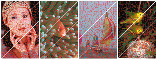
Figure 1.
Results produced by our particle-filter-based superpixel (PFS) method. The numbers of superpixels are about 300, 500, and 1000 in regions separated by two white parallel lines.
Our main contributions are the following:
- We propose a novel superpixel segmentation method based on the particle filter, which extends the original tracking problem to region clustering. Multiple particles are used to approximate superpixel centers, which could highly dispersedly be located in feature space to generate a much lower intra-cluster distance.
- Moving and perturbing processes are introduced to guide the propagation step of those particles, which reformulates the particle filter to fit our region cluster problem.
- The segmentation performance of PFS outperforms seven state-of-the-art methods on a quantitative benchmark.
2. Related Work
Graph-based methods define superpixel segmentation as the problem of searching cut edges in a graph, which could be constructed as an energy minimization problem. They describe image pixels and their similarity relationship via an undirected adjacent graph, which consists of pixel nodes and a similarity edge between adjacent pixels. Shi et al. firstly treat the pixel clustering as a graph partition called normalized cuts (NC) [10]. They consider not only intra-class similarity, but also inter-class dissimilarity, and allow regularly shaped superpixel regions to be generated. However, they employ the eigen-decomposition for the similarity matrix to approximately solve the Ncut cost function, which results in a high computational cost due to the increase in the numbers of image pixels and superpixels. Felzenszwalb et al. [11] then propose a minimum-spanning-tree-based superpixel method (FH). Instead of deleting cut edges, the method gradually adds the minimum weighted edge into the graph to generate a set of disjointed minimum spanning forests. It greedily adds edges into the graph until reaching stop conditions and significantly reduces the computational cost. However, the method generates irregular superpixel regions as the result of ignoring the compactness constraint. In order to obtain regular superpixel segmentation, Moore et al. [12,13] propose two generation methods for regular superpixel regions on the basis of horizontal and vertical lattice constraints. They model the superpixel segmentation as a node labeling problem. They either search multiple horizontal or vertical optimum paths by dynamic programming [12] or partition the graph nodes by graphcut [13]. Veksler et al. [14] utilize multiple overlapping initial patches to constrain the labeling pixel regions. This not only reduces the label space for each pixel, but also shrinks the labeling range. The authors utilize -expansion to obtain regular superpixel regions efficiently. These graph-based methods efficiently utilize combinational optimization technology to reduce the computational complexity. However, they ignore the seed location and heavily depend on similarity between adjacent nodes, which results in inferior boundary adherence. Clustering-based methods have been paid much more attention in recent years. These methods distribute initial seeds in the image evenly and update pixel labels and cluster centers alternatively until convergence. For example, Levinshtein et al. [16] propose a regular superpixel segmentation method based on constructing geometric flow with uniformly distributed seeds (TP). TP gradually evolves the boundary toward the region with the higher local gradient, which can be optimized by a level set framework [24]. However, it cannot guarantee much higher boundary adherence because of the lack of stability and efficiency for the level set method. Achanta et al. propose a popular method, SLIC [17]. The method evenly distributes initial seeds and labels each pixel on the basis of color and location distance in the constrained searched region. It updates the cluster center and pixel labels alternatively until convergence. This algorithm can maintain superpixel compactness and reduce computational cost. Benefitting from the advantage of fast K-means algorithm [17], Peng [19] and Zhang [20] also propose a higher-order energy-based method and a new distance-function-based method, respectively. The higher-order energy-based method adds a pre-segment to constrain the superpixel boundary of the SLIC on the basis of the higher-order energy, while the distance-function-based method introduces several more sophisticated distance functions to maintain superpixel compactness and boundary adherence. In addition, Shen et al. [18] integrate the compactness constraint into lazy random walks by updating seeds via the weighted average of the labeled pixels, which can generate a regular superpixel region. As a variant of SLIC, LSC [21] integrates spectral clustering and the K-means algorithm into a uniform framework, obtaining globally perceptual superpixel regions. Meanwhile, SNIC [22] introduces non-iterational clustering to enhance the connectivity of superpixel regions, which could overcome the limitation of underlying disconnected regions generated by SLIC-like methods. Most of the clustering-based methods above alternatively update initial seeds and pixel labels in an energy minimization problem. However, these methods only redefine superpixel centers as the weighted average of their corresponding pixels, instead of using much more accurate guidelines. In contrast, our method introduces particle filtering to approximate superpixel centers by multiple candidate particles. We guide the selection of cluster centers by considering the local density of pixels and the moving direction explicitly.
3. Particle Filtering
Particle filtering uses multiple weighted sample points to approximate the probability distribution, which is robust in terms of the noise background and partial occlusion. The target object can be described as . denotes all the observations up to time t. Particle filters are used to solve problems in which the posterior density and the observation density are non-Gaussian.
Particle filtering is used to approximate the probability distribution by a weighted sample set . Each sample s represents one hypothetical state of particles, with a corresponding discrete sampling probability .
The evolution of the sample set is denoted by propagating each sample according to a system model. Each element of the sample set is weighted in terms of observations, and N samples are drawn with replacement by choosing a particular sample with probability . The mean state of particles is estimated at each step by
Particle filtering provides a robust optimization framework, as it models uncertainty. It can consider multiple state hypotheses simultaneously. Inspired by its advantages, we model superpixel segmentation as a multiple-region particle filter. We treat each superpixel center as a tracking target and denote candidate centers as particles. We aim to use multiple group candidate centers (particles) to capture superpixel cores. Hence, the problem of superpixel segmentation is modeled as a multiple-region particle filtering problem.
4. Superpixel Segmentation via Particle Filtering
In this section, we introduce the particle-filter-based superpixel segmentation, which mainly consists of three steps: (1) selecting the initial particles; (2) propagating particles toward the center with lower energy cost; and (3) evaluating the observed particles on the basis of their energy cost, and selecting the lowest-energy particles as superpixel centers. The flowchart is shown in Figure 2.
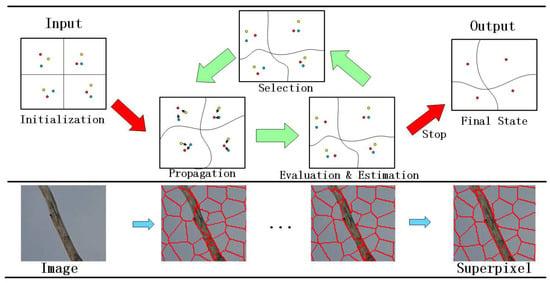
Figure 2.
The pipeline of our algorithm. Top row illustrates particle filtering processing for superpixel segmentation. Bottom row shows intermediate results at each iteration.
4.1. Problem Formulation
As superpixel segmentation is a problem of selecting the target sample set that partitions pixels in different regions, it can be described as an energy minimization problem. In terms of feature space, the distance measure can be defined to construct the energy function to assign the pixel labels into the corresponding sample. In other words, the label of each pixel depends on the minimum similarity between its feature and that of the sample component, which can be detailed as follows.
Generally, a superpixel can be intuitively presented as a color-consistent and spatially compact connected region. Thus a pixel feature can be described as a five-vector, that is, (). The pixel color is represented as to perceive the appearance similarities. The pixel position constrains the image patch with its neighboring region. For five-dimensional color and position inconsistency, the spatial distance weight is added to normalize the Euclidean distance, which effectively guarantees superpixels of similar size.
We let represent the pixel and represent the Kth sample. We calculate the distance between the image pixel and its sample component to partition the image. D is defined in Equation (2) as the five-dimensional Euclidean distance between the pixels and sample:
where the weight constraints the compactness of the superpixel. The larger is, the more compact the superpixels are. In this paper, we select to balance the color consistency and space compactness.
Then, we model the superpixel segmentation as a similarity maximization problem, which can be treated as an energy minimization as follows:
where is the association weight of data with the cluster , if , and if ; then , and the superpixel boundary will be segmented.
We constrain the pixel search range as is done in SLIC [17]. Image pixels are calculated in the region of to select their category, where , N is the number of image pixels, and K is the superpixel number. Minimizing the energy function (Equation (3)) generally introduces an expectation–maximization (EM)-style framework; that is, pixel label assignment and center updating are performed alternatively. Existing methods first evenly distribute centers into images and disturb them toward the lower-local-gradient region. Then they assign pixels to the nearest center and recalculate centers with the corresponding group pixels. However, these methods become easily stuck in the local optimum solution, which results in the inferior superpixel boundary adherence.
In order to solve this problem, we make an attempt to reduce the energy cost on the basis of particle filtering. In the next section, we detail the proposed superpixel segmentation with particle filtering.
4.2. Initial Particles’ Selection
In order to generate K superpixel regions, we initial candidate center particles in the image uniformly at fixed horizontal and vertical intervals S. Inspired by [25], the center will have a higher local density compared with its neighboring pixels. Therefore, we initialize the center particle on the basis of the density function and distance information. The distance between pixels and is denoted as , where . A radius threshold is defined to describe the density of , which is calculated by Equation (4):
where , , or otherwise ; is assigned as the average of the maximum and minimum distances among pixels. Image pixels are partitioned by applying this density function. If , is more likely as a center candidate than .
Although a particle may have the highest local density, it may not be the point with the lowest energy cost. Hence, on the basis of local density alone, one center for each superpixel region will easily become stuck in the local optimum. The lower the cost of the energy function, the higher the superpixel performance with boundary adherence. In order to obtain the segmentation with the lower energy cost, we assign multiple initial particles for each patch; this allows selection of the best center particle with the lowest energy cost. After the first group of center particles have been identified, we use the associate rule to identify the rest. They should obey the following assumptions: (1) any two candidate centers should be far away; (2) candidate centers all have a high local density. Therefore, the first center particle acts as a reference to others; is the distance between and ; and . This equation signifies that we select, as the next candidate center, the point that has a high local density and is far from the reference in region with radius ; is the weight of the distance and density function and is assigned as in this paper. Other candidate centers are selected by Equation (5):
where . This suggests that all candidate centers are far away and with high local density, as shown in Figure 3. On the interval S, the first center is assigned with the highest density in each block. Other groups are selected with the association rule. We select the next center in the region with radius . This has a high local density and is far from the existing previous center. Obeying this regularity, all candidate particles are successively obtained. We denote them as follows:
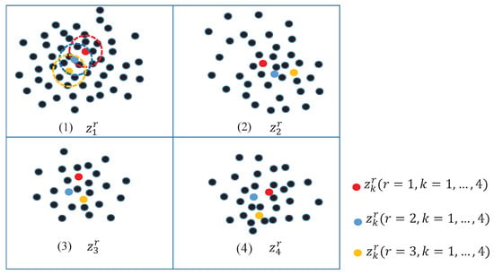
Figure 3.
Location for initial candidate particles. The data is classified into four blocks with three groups of particles. (1) The highest density is assigned as the first particle (red point); the pixel is the second particle (blue point) with the farthest distance and highest density in range of ; the particle of the third group (yellow point) is captured by the same associate rule in terms of and . Then, all particles of the first block are labeled. On the basis of the same rule, particles of blocks (2–4) can be assigned by the same rule.
On the basis of the density function and association rule, initial particles are selected. Every block contains candidate particles with a different color, but one group of particles has the same color, which is beneficial for the propagation step.
4.3. Propagation
We propagate particles toward the particle with the lower energy cost that is more likely to be the best superpixel center. We introduce movement and perturbation optimization to propagate particles.
4.3.1. Movement
For each superpixel in tth time propagation, we define the best particle as that with
Movement propagation updates other particles toward the best particle on the basis of Equation (7):
where , ; is a random number in . As shown in Figure 4, other particles move toward the best particle.
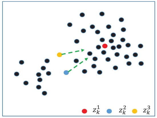
Figure 4.
Moving candidate particles toward the best particle, which is calculated with the lowest energy function. Here, and move toward the best particle with a random step.
4.3.2. Perturbation
The movement process leads to a concentrated distribution of particles. Hence, it is critical to generate diverse particles via a perturbation process. In this section, we show how other particles are perturbed toward the region with a high density distribution—except that with the lowest energy function. The process is shown in Figure 5. Specifically, particles are disturbed toward a much higher density distribution for every dimension. Given the pixels’ region of particle , the density of is defined in the following equation after tth time propagation:
where , is the mth component of , and is the mth component of , which belongs to the region of at tth time propagation; if , and otherwise. For calculating the size of the propagation step, the sum of is denoted as , or otherwise , in Equation (8).
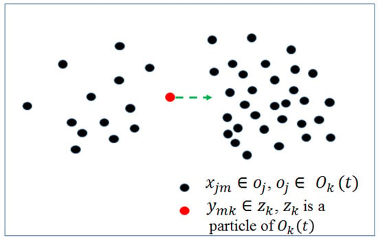
Figure 5.
Particles perturbing toward the region with much higher density distribution.
If , the density function states that of should move to the left while pixels of are concentrated in the left of . Otherwise, the density function states that of should move to the right while pixels of are concentrated in the right of .
Here, represents the difference between the particle component and average pixels located in its right region.
Here, represents the difference between the particle component and average pixels located in its left region.
4.4. Evaluation and Estimation
In the evaluation step, we calculate the energy cost for each group of particles via Equation (3). Then, in the estimation step, we need to identify the superpixel center, that is, the best group, to complete the segmentation task. It is clear how to identify the best candidates from the particle group with the lowest energy cost. This will lead to more tightness in the region clustering in terms of feature space. The iteration will terminate when the stop conditions are satisfied.
Our superpixel generation algorithm (Algorithm 1) is shown as follows.
| Algorithm 1 Algorithm for PFS. |
Require:
|
4.5. Selection
In the tracking problem, the selection step aims at redistributing the samples according to their weights. A sample with a large weight may be selected more frequently. Others with relatively low weights may be chosen with fewer opportunities or not at all. This could save computing resources. In our problem, we aim to relocate the best particle group in the selection step to propagate these particles with a clearer direction. Thus, we propose a crossing process to complete the particle selection.
The best observed particle group obtained by propagation is that with the lowest energy cost among the candidate particles. However, it may not have the minimum intra-cluster distance in each group. Our aim is to exchange particles in different groups. Specifically, we replace the best center particle with that which has the minimum intra-cluster distance among the candidates, as described in Equation (11). Then, selected particles recombine into a new group, which would further decrease Equation (3).
The crossing selection is shown in Figure 6. The best particle group (square) is generated at the tth iteration. Particles with different shapes belong in different groups. Icons with the same shape describe particles in the same group for superpixels. This shows that the intra-cluster distance of each best center particle does not make it minimal in the category. For example, the blue disk has the minimal intra-cluster distance in the second group (second column) and would be moved into the first group after this process. After updating pixel labels, Equation (3) would be decreased again.
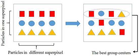
Figure 6.
Crossing selection. Particles in the same row represent centers in different superpixels. Particles in the same column denote different candidate centers in one superpixel. Particles in the first group are the best group centers for image superpixels.
5. Experiment
In order to evaluate the proposed method, we performed our method on the Berkeley segmentation 500 dataset (BSD500). Five hundred natural images are contained in this dataset. We also compared seven state-of-the-art superpixel algorithms with our method: NC [10], TP [16], FH [11], SLIC [17], LSC [21], Regularity preserved superpixels (RPS) [26] and SNIC [22]. We ran segmentation code of these methods, which was made available by the authors.
5.1. Performance Evaluation
Superpixel algorithms have different evaluation criteria with image segmentation. The common metrics are under-segmentation error (UE) [27], boundary recall (BR) [28], and achievable segmentation accuracy (ASA) [29]. We use to denote the segmentation of ground truth and use to represent results of superpixel algorithms.
(1) Boundary recall: BR is described as the contact ratio of ground truth boundaries that fall within the nearest superpixel boundaries. The best superpixel segmentation algorithm has a good ability to adhere well to object boundaries.
where and represent the superpixel region and ground truth. A high value of BR indicates that the segmentation result overlaps with the ground truth and very few true edges were missed. From the BR measurement, our superpixel algorithm outperformed all state-of-the-art methods and produced an increasing superpixel number, as shown in Figure 7, particularly at a lower density. In terms of the BR rate, for 100 superpixels, our method outperformed the best method among all compared methods, that is, SNIC [22], by almost 3%. The reason is that our method can use multiple candidate particles efficiently to approximate superpixel centers with a much higher regional consistency. It also benefits from the guidance of our propagation and selection steps, which alleviate the risk of the energy cost becoming stuck into local optimum. However, SNIC [22] updates its centers on the basis of weighting average pixel members and tends to stop at the local optimum.

Figure 7.
Performance evaluation in terms of boundary recall (BR), under-segmentation error (UE) and achievable segmentation accuracy (ASA).
(2) Under-segmentation error: To map the image boundary, a superpixel only overlapping one object is used to evaluate the segmentation method. A better superpixel generation algorithm would try to avoid the under-segmentation areas. This error is computed in terms of the bleeding of the superpixel region over ground truth and is used to penalize the superpixel that could not be aligned to the ground truth boundary tightly. The formula is expressed by
where N is the total number of pixels, and is the area of the superpixel . Lost pixels are denoted as . Then, B represents the minimum area of overlapping. In our experiment, the value of B was of . A lower UE represents that fewer superpixels straddle over multiple object regions. In other words, irregular superpixels tend to yield a higher UE. Figure 7 gives the UE of superpixel segmentation by the compared methods. It can be seen that our method outperformed the compared state-of-the-art methods. This demonstrates that our superpixels not only had high boundary adherence, but also had regions of regular and compact shape.
(3) Achievable segmentation accuracy: This measure evaluates whether the object is recognized [29] and computes the highest achievable accuracy by overlapping the area of the superpixel with ground truth; the method is defined by
A higher ASA signifies that more objects are recognized correctly in an image. The value of the ASA was calculated by averaging all of the images in the BSD500 and plotting against the number of superpixels, as shown in Figure 7. Our algorithm outperformed the compared methods and generated the most correct overlapping regions, which had the same label, shared between superpixels and ground truth. In particular, along with the increasing numbers of superpixels, our method obtained higher segmentation performance. This suggests that multiple particles could more easily approximate superpixel centers with higher regional consistency under dense superpixel conditions.
We also discuss the effect of the number of particles. The BR for different particles numbered under 100, and 500 superpixels are shown in Table 1. It can be seen that the performance increased with the increasing of the particle number. PFS obtained the best BR for five particles. Meanwhile, the performance tended to be stable when . This was because it is difficult to converge few particles for the same region to the lowest energy cost. Oppositely, more particles associated with the same local region will converge to the same optimal solution. In order to obtain balance between the performance and runtime, we selected the particle number in our experiments.

Table 1.
The effect of particle number in terms of boundary recall.
We selected five particles in our method and compared the runtime with that of the state-of-the-art methods for 200 superpixels with on an Intel 2.33 GHz CPU with a 4 GB RAM desktop. The time is shown in Table 2. It suggests that our method obtains comparable running times to the state-of-the-art methods. However, the multiple groups of particles with perturbation and crossing increase the running time.

Table 2.
Average running time (seconds per image).
5.2. Visual Comparison
Figure 8 shows some subjective results for the proposed PFS method. It can be seen that our method has several advantages, as follows: (1) It obtains high object-boundary adherence; (2) it maintains a fine structure of the object boundary; (3) it generates a regular and compact superpixel region. Specifically, for the duck image, the duck has a similar appearance to the sky, particularly for the wings. Our method can extract the region boundary between these well and yields less region leakage, which verifies the ability for weak boundary preserving of the PFS. Furthermore, for the branches, our method also maintains the region boundary, which demonstrates that our method can preserve the fine structure of the object region. This is because multiple-PFS segmentation can efficiently locate seeds in long and narrow object regions, making it superior to regular lattices or local-gradient-perturbation-based seed-location methods. In addition, our method can yield regular and compact superpixels even in the clutter background. In short, these advantages verify our method’s robustness and efficiency.
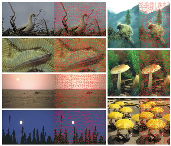
Figure 8.
Some subjective results for our particle-filter-based superpixel (PFS) segmentation.
Figure 9 shows some subjective results compared between our method and seven state-of-the-art methods. As can be seen, PFS outperformed all compared methods in the complex and clutter background. For example, for the bird image, in order to adhere to the boundary of the wing region, FH [11] pays the price of losing regularity. Although other seed-based methods [16,17,21,22] generate regular and compact superpixels, they yield superpixels with high UE. However, our method not only fits the wing’s boundary better than other methods, but also generates regular and compact superpixels in the clutter sky and ocean background. This suggests that our method could adaptively fit the object boundary, that is, reduce regularity to fit the irregular object parts and generate compact superpixels in relatively smooth regions. This is because our method can use multiple particles to accurately locate different object regions, which generates superpixels with consistent appearance features. The insight into this idea is that, for example, the more dispersed the superpixel centers are, the better the boundaries’ adherence. In contrast, other seed-based methods only coarsely locate their seeds in uniform lattices and adjust the center position locally. This increases the risk of centers losing locations of irregular object regions, which results in a high UE. For RPS [26], it is also hard to accurately locate the junction of superpixel borders on the object boundary. It can be seen that RPS yields a higher segmentation error. These compared results demonstrate that our method can adaptively adjust region regularity and boundary adherence even in the clutter background and complex object shape. This is a benefit of our multiple-particle-filtering framework, particularly the propagation and selection steps.
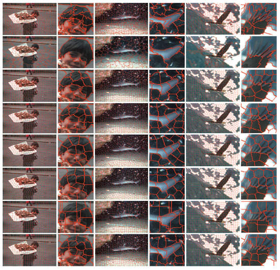
Figure 9.
Visual comparison between our algorithm and other algorithms. From top to bottom, results were processed by our algorithm, FH [11], simple linear iterative clustering (SLIC) [17], TurboPixels (TP) [16], normalized cuts (NC) [10], LSC [21], RPS [26], and SNIC [22].
6. Conclusions
In this paper, we propose a novel superpixel segmentation method based on particle filtering, which extends the original tracking problem to multiple-region clustering. The basic idea is to approximate superpixel centers by multiple particles to obtain greater intra-region similarity. Toward this goal, we use a density cluster and associate rule to mine initial candidate particles. Then, particles are transferred to neighboring local regions with lower energy cost in the propagation step. We evaluate all particles on the basis of their cluster similarity and estimate the largest as the final superpixel centers. The proposed method can alleviate the risk of a local optimum and obtain a better segmentation performance. Meanwhile, PFS has the ability of adaptively adjusting regions’ regularity and boundary adherence even in the clutter background and complex object shape. Experimental results on the BSD500 segmentation dataset demonstrate that our method outperformances seven state-of-the-art methods.
Author Contributions
L.X. and B.L. conceived and worked together to this paper. L.X. compiled the computing program by Matlab and analyzed the data. B.L. compiled some subfunctions by C Mex files. Z.P. and K.Q. pointed out some key steps and reformulated the formulas.
Acknowledgments
This work is supported by the Typical Spectrum of Radio Signal (szjj2016-092) and the National Natural Science Foundation (61372187 and 61473239).
Conflicts of Interest
The authors declare no conflict of interest.
References
- Han, B.J.; Sim, J.Y. Saliency Detection for Panoramic Landscape Images of Outdoor Scenes. J. Vis. Commun. Image Represent. 2017. [Google Scholar] [CrossRef]
- Xiao, Y.; Wang, L.; Jiang, B.; Tu, Z.; Tang, J. A global and local consistent ranking model for image saliency computation. J. Vis. Commun. Image Represent. 2017, 46, 199–207. [Google Scholar] [CrossRef]
- Fareed, M.M.S.; Ahmed, G.; Chun, Q. Salient region detection through sparse reconstruction and graph-based ranking. J. Vis. Commun. Image Represent. 2015, 32, 144–155. [Google Scholar] [CrossRef]
- Zhu, H.; Meng, F.; Cai, J.; Lu, S. Beyond pixels: A comprehensive survey from bottom-up to semantic image segmentation and cosegmentation. J. Vis. Commun. Image Represent. 2016, 34, 12–27. [Google Scholar] [CrossRef]
- Fulkerson, B.; Vedaldi, A.; Soatto, S. Class segmentation and object localization with superpixel neighborhoods. In Proceedings of the 2009 IEEE 12th International Conference on Computer Vision, Kyoto, Japan, 29 September–2 October 2009; pp. 670–677. [Google Scholar]
- Luo, B.; Li, H.; Song, T.; Huang, C. Object segmentation from long video sequences. In Proceedings of the 23rd ACM International Conference on Multimedia, Brisbane, Australia, 26–30 October 2015; pp. 1187–1190. [Google Scholar]
- Uijlings, J.R.; Van De Sande, K.E.; Gevers, T.; Smeulders, A.W. Selective search for object recognition. Int. J. Comput. Vis. 2013, 104, 154–171. [Google Scholar] [CrossRef]
- Mori, G.; Ren, X.; Efros, A.A.; Malik, J. Recovering human body configurations: Combining segmentation and recognition. In Proceedings of the 2004 IEEE Computer Society Conference on Computer Vision and Pattern Recognition, Washington, DC, USA, 27 June–2 July 2004; Volume 2, pp. II-326–II-333. [Google Scholar]
- Yuan, Y.; Fang, J.; Wang, Q. Robust Superpixel Tracking via Depth Fusion. IEEE Trans. Circuits Syst. Video Technol. 2014, 24, 15–26. [Google Scholar] [CrossRef]
- Shi, J.; Malik, J. Normalized cuts and image segmentation. IEEE Trans. Pattern Anal. Mach. Intell. 2000, 22, 888–905. [Google Scholar]
- Felzenszwalb, P.F.; Huttenlocher, D.P. Efficient Graph-Based Image Segmentation. Int. J. Comput. Vis. 2004, 59, 167–181. [Google Scholar] [CrossRef]
- Moore, A.P.; Prince, S.J.D.; Warrell, J.; Mohammed, U.; Jones, G. Superpixel lattices. In Proceedings of the 2008 IEEE Conference on Computer Vision and Pattern Recognition, Anchorage, AK, USA, 23–28 June 2008; pp. 1–8. [Google Scholar]
- Moore, A.P.; Prince, S.J.; Warrell, J. Lattice Cut—Constructing superpixels using layer constraints. In Proceedings of the 2010 IEEE Conference on Computer Vision and Pattern Recognition (CVPR), San Francisco, CA, USA, 13–18 June 2010; pp. 2117–2124. [Google Scholar]
- Veksler, O.; Boykov, Y.; Mehrani, P. Superpixels and Supervoxels in an Energy Optimization Framework. In Proceedings of the Computer Vision—ECCV 2010: 11th European Conference on Computer Vision, Heraklion, Greece, 5–11 September 2010; Part V. Springer: Berlin/Heidelberg, Germany, 2010; pp. 211–224. [Google Scholar]
- Meng, F.; Li, H.; Wu, Q.; Luo, B.; Huang, C.; Ngan, K. Globally Measuring the Similarity of Superpixels by Binary Edge Maps for Superpixel Clustering. IEEE Trans. Circuits Syst. Video Technol. 2016, 28, 906–919. [Google Scholar] [CrossRef]
- Levinshtein, A.; Stere, A.; Kutulakos, K.N.; Fleet, D.J.; Dickinson, S.J.; Siddiqi, K. TurboPixels: Fast Superpixels Using Geometric Flows. IEEE Trans. Pattern Anal. Mach. Intell. 2009, 31, 2290–2297. [Google Scholar] [CrossRef] [PubMed]
- Achanta, R.; Shaji, A.; Smith, K.; Lucchi, A.; Fua, P.; Susstrunk, S. SLIC Superpixels Compared to State-of-the-Art Superpixel Methods. IEEE Trans. Pattern Anal. Mach. Intell. 2012, 34, 2274–2282. [Google Scholar] [CrossRef] [PubMed]
- Shen, J.; Du, Y.; Wang, W.; Li, X. Lazy Random Walks for Superpixel Segmentation. IEEE Trans. Image Process. 2014, 23, 1451–1462. [Google Scholar] [CrossRef] [PubMed]
- Peng, J.; Shen, J.; Yao, A.; Li, X. Superpixel Optimization Using Higher Order Energy. IEEE Trans. Circuits Syst. Video Technol. 2016, 26, 917–927. [Google Scholar] [CrossRef]
- Zhang, Y.; Li, X.; Gao, X.; Zhang, C. A Simple Algorithm of Superpixel Segmentation with Boundary Constraint. IEEE Trans. Circuits Syst. Video Technol. 2017, 27, 1502–1514. [Google Scholar] [CrossRef]
- Li, Z.; Chen, J. Superpixel segmentation using linear spectral clustering. In Proceedings of the IEEE Conference on Computer Vision and Pattern Recognition, Boston, MA, USA, 7–12 June 2015; pp. 1356–1363. [Google Scholar]
- Achanta, R.; Süsstrunk, S. Superpixels and Polygons using Simple Non-Iterative Clustering. In Proceedings of the IEEE Conference on Computer Vision and Pattern Recognition, Honolulu, HI, USA, 21–26 July 2017. [Google Scholar]
- Nummiaro, K.; Koller-Meier, E.; Van Gool, L. An adaptive color-based particle filter. Image Vis. Comput. 2003, 21, 99–110. [Google Scholar] [CrossRef]
- Malladi, R.; Sethian, J.A.; Vemuri, B.C. Shape modeling with front propagation: A level set approach. IEEE Trans. Pattern Anal. Mach. Intell. 1995, 17, 158–175. [Google Scholar] [CrossRef]
- Rodriguez, A.; Laio, A. Clustering by fast search and find of density peaks. Science 2014, 344, 1492–1496. [Google Scholar] [CrossRef] [PubMed]
- Fu, H.; Cao, X.; Tang, D.; Han, Y.; Xu, D. Regularity preserved superpixels and supervoxels. IEEE Trans. Multimed. 2014, 16, 1165–1175. [Google Scholar] [CrossRef]
- Yao, J.; Boben, M.; Fidler, S.; Urtasun, R. Real-Time Coarse-to-Fine Topologically Preserving Segmentation. In Proceedings of the IEEE Conference on Computer Vision and Pattern Recognition (CVPR), Boston, MA, USA, 7–12 June 2015. [Google Scholar]
- Arbelaez, P.; Maire, M.; Fowlkes, C.; Malik, J. Contour Detection and Hierarchical Image Segmentation. IEEE Trans. Pattern Anal. Mach. Intell. 2011, 33, 898–916. [Google Scholar] [CrossRef] [PubMed]
- Comaniciu, D.; Meer, P. Mean shift: A robust approach toward feature space analysis. IEEE Trans. Pattern Anal. Mach. Intell. 2002, 24, 603–619. [Google Scholar] [CrossRef]
© 2018 by the authors. Licensee MDPI, Basel, Switzerland. This article is an open access article distributed under the terms and conditions of the Creative Commons Attribution (CC BY) license (http://creativecommons.org/licenses/by/4.0/).