1. Introduction
Multiple-input multiple-output (MIMO) radar technology was formally introduced in 2004 [
1]. The concept of MIMO radar is widely used in various military and civilian equipment. It has attracted much attention due to its high positioning accuracy, low-speed moving-target detection performance, and very low interception probability [
2,
3,
4]. At the receiving end of MIMO radar, each receiving element receives all the transmitted signals and acquires multiple echo signals by matching the filter after signal processing of clutter filtering.
MIMO radar can detect targets by transmitting multiple orthogonal signals. The mutual coupling phenomenon is obvious between the MIMO radar antenna array elements if the element distance is too close. Therefore, in order to ensure the orthogonality between MIMO radar multiple channels, it is necessary to maintain sufficient distance between the radar antenna elements, which is difficult for installation because of the bulkiness and expensiveness of a MIMO radar system. In addition, there are still many problems with civilian MIMO radar applications, such as automobile radar, which has poor robustness of output waveform and an obvious multipath effect [
5]. In order to solve a series of problems caused by a large transmitting array, a sparse array method was adopted to simplify the hardware composition of the MIMO radar system [
6]. However, this method will lead to an increase in the side lobe level of MIMO radar, which needs to be optimized by various algorithms to offset the side lobes without changing the size of MIMO radar. The genetic algorithm (GA), particle swarm optimization (PSO), least squares algorithm (LS), and other traditional intelligent algorithms have been previously derived to meet the requirements of antenna array distribution [
7,
8,
9,
10].
As one of the important aspects of array signal processing, direction of arrival (DOA) has been widely used in many fields, such as radar, communication, sonar, seismic exploration, radio astronomy, and biomedical engineering. Multiple signal classification (MUSIC) and estimation rotational parameter via rotational invariance (ESPRIT) are two typical algorithms used for estimating the DOA. The classic process used for MUSIC performance analysis in DOA estimation is illustrated in [
11], where high signal-to-noise (SNR) maximum-likelihood estimator (MLE) performance was obtained. Two methods of image generation from multistatic data were analyzed in [
12], and the MUSIC method adopted the singular vectors having small or zero singular values. The performance of time-reversal (TR) MUSIC for computational TR applications was studied in [
13] to give a theoretical analysis of MUSIC for DOA estimation. In [
14], a combined signal parameter unitary estimation by an ESPRIT-based algorithm was used to optimize the DOA of MIMO radar. However, the genetic algorithm has limitations: it easily falls into the local extremum and cannot find the optimal solution. The DOA estimation for MIMO radar with mutual coupling is also addressed in [
15,
16]. The reweighted sparse representation algorithm based on noncircular sources was suggested to provide higher resolution and better angle estimation performance than ESPRIT algorithm. A pilot pattern algorithm based on the least squares (LS) algorithm for channel estimation in MIMO-orthogonal frequency division multiplexing (OFDM) systems is discussed in [
17]. The joint smoothed
l0-norm algorithm for fast sparse DOA estimation has been proposed for multiple measurement vectors in MIMO radar systems [
18]. The results indicated that it can eliminate the white or colored Gaussian noises and achieve better DOA estimation performance. The nuclear norm minimization algorithm [
19] was proposed to extend the virtual array aperture, which provides better performance compared with the conventional sparse recovery-based algorithms and can handle the case of underdetermined DOA estimation in MIMO radar systems. The single-link MIMO system was originally developed on the basis of virtual array elements. Different methods to realize the physical structure of the single radio frequency (RF) link radar receivers are discussed in [
20]. The single RF link MIMO transmission system was investigated more systematically in [
21]. The antenna feed terminal entity element in the MIMO system was replaced by a virtual antenna element, and the transmitter array was more efficient by using the binary phase shift keying (BPSK) modulation. This technique not only solves the size problem of MIMO antennas, but reduces the mutual coupling between antennas, which greatly improves the efficiency of MIMO systems. The single RF link MIMO-OFDM system was proposed [
22,
23,
24] to realize the purpose of multicarrier signal transmission. Several signals were superimposed in the time domain and the OFDM waveform was finally formed. This solves the problem of replication interference caused by the beam switching in the receiver of MIMO antennas compared to the previous systems. A beam-switched antenna was realized by using eight parasitic antenna elements and PIN diodes, which effectively met the demand of generating more waveforms at the transmitter. A compact frequency tunable single RF link MIMO transmission scheme was proposed in [
25]. This approach simplifies the DC bias circuit and various loads in the BPSK modulation, so the external reconfigurable matching circuits can be omitted for simplification.
A virtual array is created by sending independent waveforms from the transmitting array to the receiving array, which improves the degrees of freedom of phased array and MIMO systems. This kind of MIMO radar reduces false alarms and increases its robustness to noise [
26]. Traditional algorithms are usually applied in the ideal sparse environment, however, MIMO radar signals are not sparse enough in the time and frequency domains. Therefore, the time frequency ridge estimation algorithm was proposed [
27] to improve the reconstruction accuracy of MIMO radar signals. To suppress the high grating lobes in the near-field imaging results in MIMO synthetic aperture radar array, the relationship between the target’s point spread function and the transmitter/receiver (T/R) array pattern was studied, and the proper height of the T/R arrays was adjusted to focus on the near-field edge points perfectly [
28,
29,
30,
31].
A colocated algorithm was presented for distributed MIMO radar systems in [
32]. In order to estimate the location parameter, range sum measurements were performed to determine the distance between the receiver and the target. As for the single RF link MIMO radar, it can achieve a similar performance for the same target distance with a small detection error rate. Besides, considering the simplicity and cost-effective advantages, it is a good candidate for wireless communications.
In this work, using the switch parasitic antenna as the carrier, the single RF link MIMO radar was studied to realize the traditional MIMO measurement ability of velocity and range. Based on the single RF link technology, the MIMO radar antenna was optimized to achieve better system performance. A simulation platform was established to verify the method and the correctness of single RF link MIMO theory. Several important modules of the single RF link MIMO radar system will be introduced, and the differences between the single RF link MIMO radar system and the conventional MIMO radar system will be discussed in detail.
The remainder of the paper is organized as follows.
Section 2 describes the working principles of MIMO radar, combining the single RF link chain with the MIMO system.
Section 3 introduces the establishment of single RF link MIMO radar simulation platform and gives the implementation method for each part of the MIMO system. The main factors that influence the single RF link MIMO radar performance are discussed in
Section 4. A method based on the simulation results is put forward to increase the system robustness. Finally, the conclusion is given in
Section 5.
Main notations in this paper:
| (·)H: Conjugate transpose | G(·): Gamma distribution |
| U(x): unit step function | Kv(·): v order Bessel function |
| J0 (·): zero order Bessel function | E[·]: expected operation |
2. MIMO Radar Principle
The complexity of the MIMO radar system is a major impediment to its development of wide applications. The cost of the RF chains and power consumption is increased by the number of the antenna element arrays. For such circumstances, a MIMO system with a single RF link chain is proposed, which not only reduces the dimensions and cost, but shows better performance compared to the traditional complex MIMO system.
A single RF link MIMO radar first generates a control signal through two random digital signals. One of the signals is the control signal of the initial orthogonal basis, and the result obtained by the two signal XOR operations controls the opening direction of the single pole double throw(SPDT) switch. Assuming that
and
represent the projection of the two orthogonal digital signals of the scatter directions [
33,
34], the virtual channel representation can be expressed as:
where
and
will be determined by the virtual angles
and
. The matrix
represents the complex gain between different transmitting and receiving patterns of the MIMO channel.
As for the single RF MIMO transmitter, the transmitting version pattern can be described as:
can be considered as the sampled transmitting pattern of the MIMO radar. As for the single receiver port, it is not possible to realize the spatial sampling of the incident wave.
Neff denotes the number of the symbol period division for different patterns. The received vector at the end of the period can be described as:
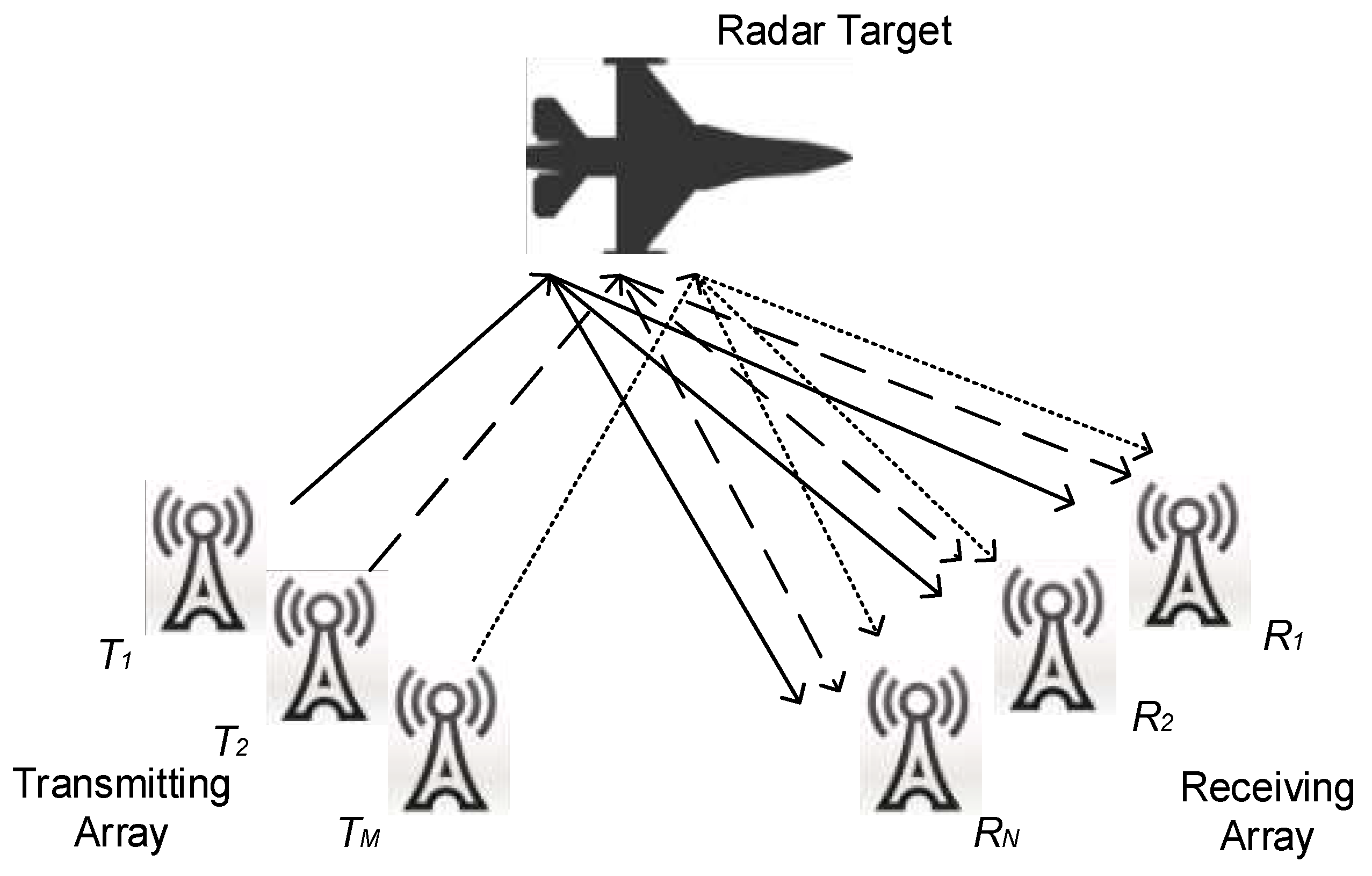
The MIMO radar system adopts a series of transmitting antennas to construct orthogonal signals in the time domain and transmits them to air space at the same time. The reflection on the target of the electromagnetic wave is received by multiple antennas at the receiver. The space position and motion state information of the target are extracted by a comprehensive process of the reflection wave. A schematic diagram of MIMO radar is shown in
Figure 1. The whole MIMO radar system consists of
M transmitting antennas and
N receiving antennas. The
M transmitting antennas can work simultaneously to transmit orthogonal signals and the
N receiving antennas can receive all the target echoes simultaneously, thus forming
M ×
N observation channels. The introduced observation channels are far more than the actual number of physical array elements and, ultimately, multichannel information acquisition capability is realized using this method. Accordingly, the multiple MIMO RF links make signal processing more complicated than traditional radar.
False alarm is the phenomenon that occurs when, even if there is no signal at the input of the radar receiver, it still judges that the signal existed. Since radar performance has always been affected by outside interferences, such as sea surface and internal receiver thermal noise, it is necessary for radar to acquire a certain signal-to-noise ratio (SNR) when extracting a signal from the received waveform. As for the adaptive detection algorithms for radar targets, two adaptive detectors were proposed in [
35], which eliminated the need for matched filtering for colocated MIMO radar target detection. In [
36], the persymmetric generalized likelihood ratio test (PGLRT) for distributed MIMO radar was studied, which has a simpler form and a more efficient computation process. The problem of adaptive multichannel signal detection in homogeneous Gaussian disturbance was discussed in [
37]. In the current work, the cell-averaging constant false alarm rate (CA-CFAR) was adopted to correct the adverse effect caused by false alarm detection. The advantages of CFAR are that it can adjust the detection threshold adaptively according to the characteristics of the reference window and, besides, the false alarm probability is low compared to other algorithms.
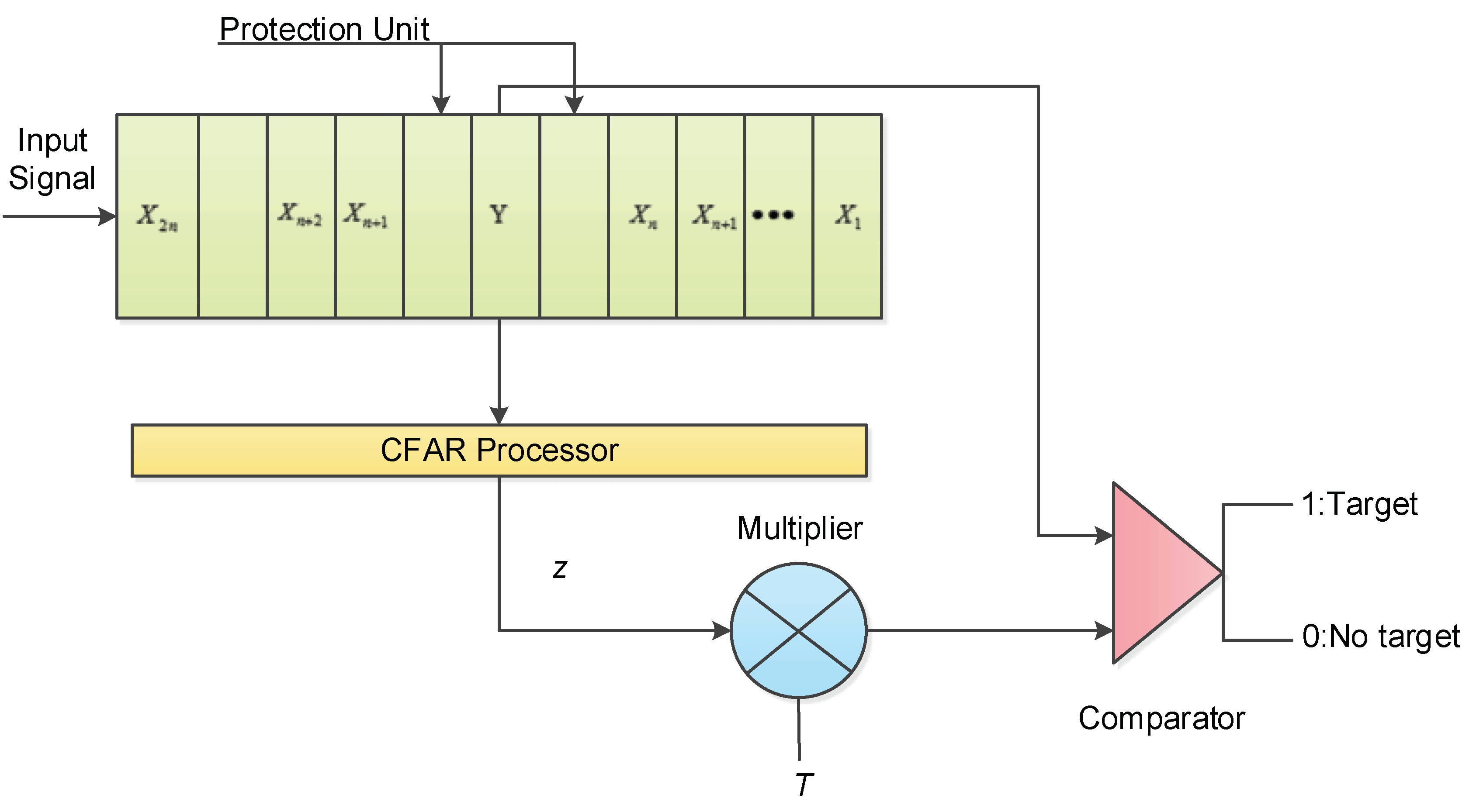
There are many CFAR detection algorithms, such as the element averaging method and the element maximum method.
Figure 2 illustrates the classic CA-CFAR algorithm process. The protection unit plays a role in preventing the target energy from leaking to the sides of the unit, which is generally used in the single-target case. There are
n signals on both sides of the protection unit, used as the reference unit, and
Y is called the detection unit. Clutter level estimation
Z is obtained by processing the reference unit via the CFAR processor. After being multiplied with the normalized factor
T, it enters into the comparator for comparison. If the result is higher than
T×
z, it indicates that the target is found; if it is below, the target is not found.
K distribution is a recognized hybrid model that reflects the radar clutter characteristics. The probability density function of the
K distribution is shown in (4):
U(
x) represents the unit step function and
Kv(·) is the
v order Bessel function of the second kind.
v and
a denote the shape coefficient and scaling factor, respectively. For a variable
θ that is uniformly distributed between 0 and 2π, the characteristic function
CY (
u;
v) can be defined as:
J0 (·) and
E[·] represent the zero-order Bessel function expected operation. When the second Bessel function approaches infinity, the characteristic function
CY (
u;
v) has a limited value:
If the limit can be expressed as (7), then we can get (8):
Therefore, when the order tends to infinity, the distribution is changed into Rayleigh distribution.
In particular, if we set
v =
n + 0.5, then the second kind of Bessel function can be expressed as:
Assuming
G(
y;
a,
i) is the Gamma distribution of
a and
i:
If we plug (10) into (4), we obtain:
When we integrate x on both sides of (12), we obtain (14).
According to (13), every element in the sequence {
αi = 2, …,
n + 2} is non-negative, which means the variables of Rayleigh distribution can be considered as a mixture of several two-dimensional χ
2 distribution variables. Defining a sequence of weights {
p1(
i);
i = 0, 1, 2, …}, where
p1(
i) =
αi when
i = 2, 3, 4, …,
n + 2 and
p1(
i) = 0 when
i takes other values, then we can express (11) as:
The polynomial coefficient sequence {pm(i); i = 0, 1, 2, …} is obtained after M times convolution of itself, which means pm(i) = pm−1(i)* p1(i) and the coefficient sequence can be obtained by the fast Fourier transformation (FFT) algorithm.
3. MIMO Radar Simulation Platform
This section introduces the structure of the traditional MIMO radar simulation platform, and then compares the performance of the MIMO radar simulation platform with the MIMO radar simulation platform optimized by the single RF link.
The composition of a MIMO radar system is complex and can be divided into several modules, including the signal generation module, the target module, the channel module, the signal receiving module, and the data analysis module. The structure of the traditional MIMO radar simulation platform is shown in
Figure 3.
In the signal generation module and receiving module, an antenna array is used for transmitting and receiving. The signal-processing module includes filtering, frequency conversion, and demodulation processes. For different kinds of applications, it may employ the FFT principle, pulse compression, space-time adaptive processing, and intelligent algorithm. The data analysis process uses various algorithms to obtain the target distance, velocity, detection probability, and other physical quantities. The final processing results are obtained to complete the whole radar detection process.
3.1. Signal Generation Module
MIMO radar uses a linear frequency modulation (LFM) as a transmitting signal. The
PRI,
β, and
τ parameters represent the pulse repetition interval, signal pulse bandwidth, and pulse width, respectively. The time domain LFM signal is shown in
Figure 4. It can be expressed as:
LFM signal can be categorized as a wide time bandwidth signal and can meet the demand of pulse compression technology. According to the theory of signals and systems, the time width of the signal is inversely proportional to the bandwidth, and the product of the two physical quantities is fixed. LFM signaling is widely used because of its simplicity, convenient processing, and mature technology. In order to adapt to different circumstances, the pulse repetition interval of the LFM signal can also be non-uniform. Correspondingly, additional processing is required at the receiver and the algorithm is more complex. In this paper, we will discuss the performance of single RF link MIMO radar with a uniform pulse repetition interval LFM signal.
3.2. Noise and Data Receiver Module
Radar targets can reflect electromagnetic waves in space. For different kinds of radar targets, the characteristics of the reflected signals are different. Generally, the radar cross-section (RCS) is used to measure the characteristics of the target.
The σ, A, and λ parameters represent the radar target RCS, the irradiated area, and the operating wavelength of radar, respectively. For most complex scattering targets, RCS represents the equivalent area. The larger σ is, the more likely the target is to be detected by radars. For the opposite condition, it is not easily detected and has excellent stealth performance.
If the RCS of targets in the same processing cycle is constant, and different treatment periods are not related to each other, then the radar target falls into the slow fluctuating category; if the pulses are not related to each other, the radar target falls into the rapidly fluctuating category. If the target has no fluctuation characteristics, it is called a “no fluctuation target” (also called Swerling 0 type). The radar targets can be roughly divided into four categories according to the type of the fluctuating target and their respective probability density functions, as is shown in
Table 1.
The five radar targets correspond to different target types. In general, Swerling I and II apply to the approximately equal scattering targets at low speed and high speed, respectively. Swerling III and IV apply to the strong dispersion and a plurality of small reflecting targets at low speed and high speed, respectively. Swerling 0 type corresponds to the target in uniform linear motion. In this study, the radar target focused on was the Swerling 0 type, and the rest of the targets were obtained by modifying the target type in the software.
In the MIMO radar receiver, the received signal is not only reflected by the target signal, but interfered with by all kinds of noise and clutter. They can be divided into external noise and the internal noise. External noise is mainly caused by the interference from external electromagnetic waves, such as discharge phenomena. Internal noise is mainly caused by materials or internal circuits affects, such as thermal noise. A noise signal can be classified as additive noise and multiplicative noise according to its attributes. Thermal noise and shot noise belong to the additive noise category.
If the source signal and the noise signal are represented as s(t) and n(t), then the noise signal is usually expressed in the form of s(t) + n(t). In the process of establishing the system platform, the additive noise is generally regarded as the background noise of the system. Channel-fading and the noise generated by the nonlinear system are multiplicative noise, which is generally expressed in the form of s(t) × [1 + n(t)]. If the source signal disappears, then the multiplicative noise has no effect on the system. The noise and interference in this paper are all additive.
In this work, the interference module adopted the Rayleigh noise, which is mainly used to describe the statistical laws of the flat fading signals. The envelope of the Rayleigh noise distribution is the sum of the Gaussian noise signal envelopes of two orthogonal distributions. The probability density function is:
For the actual work environment, the radar signals will always be interfered with by other clutter when the working environment changes, including natural clutter such as the ground and waves, or artificial clutter such as chaff, corner reflectors, and so on. The noise type can be adjusted according to the requirements of different radar application environments.
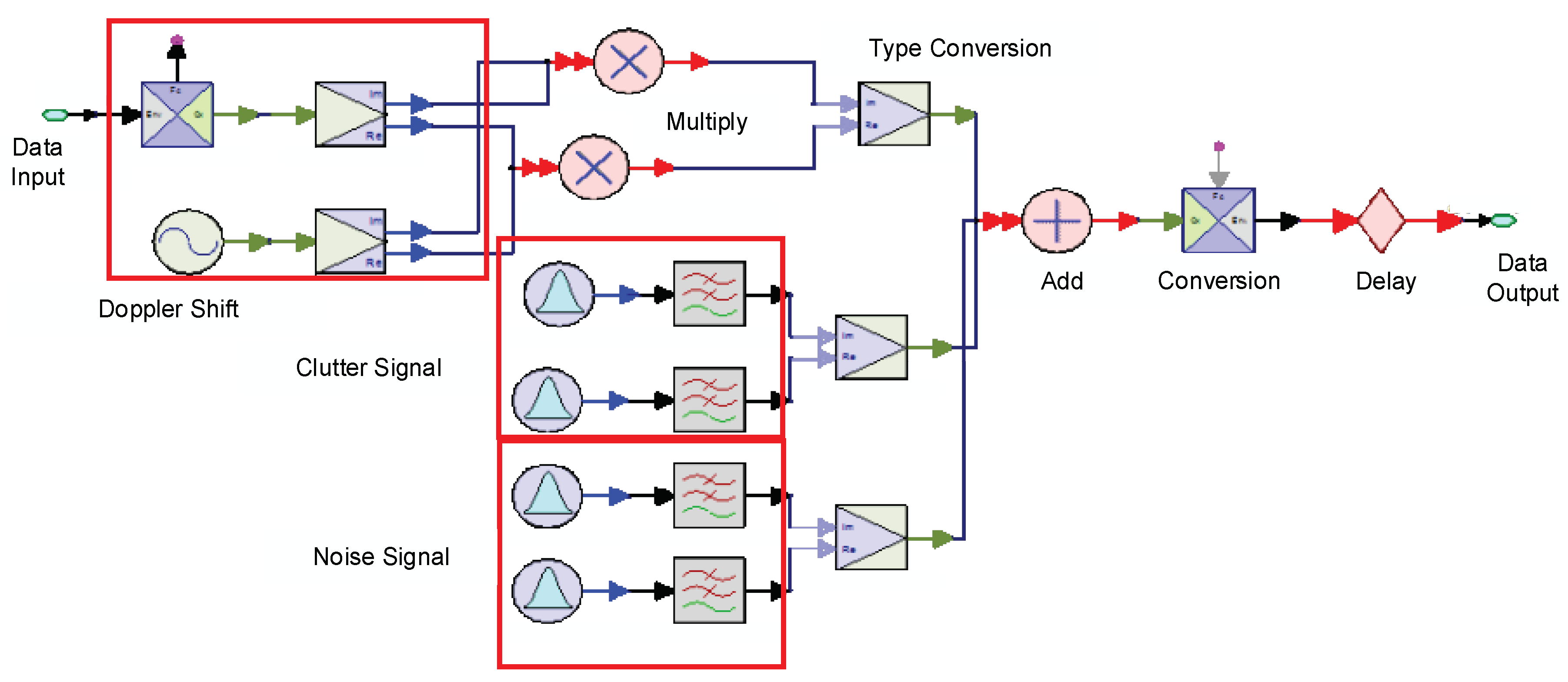
As can be seen from
Figure 5, the signal generated in the previous step is multiplied with a complex signal in the real part and the imaginary part, respectively. The complex signal amplitude is 1 V, and the frequency
Fd is the Doppler shift of the radar target. The clutter and noise of the Rayleigh distribution are generated by Gaussian signal generator. The difference is that the bandwidth is different from the amplitude. After the superposition, the target delay is added by a delay element and the distance of the target can be calculated. The resulting signal is a reflected signal with clutter, noise, and target information.
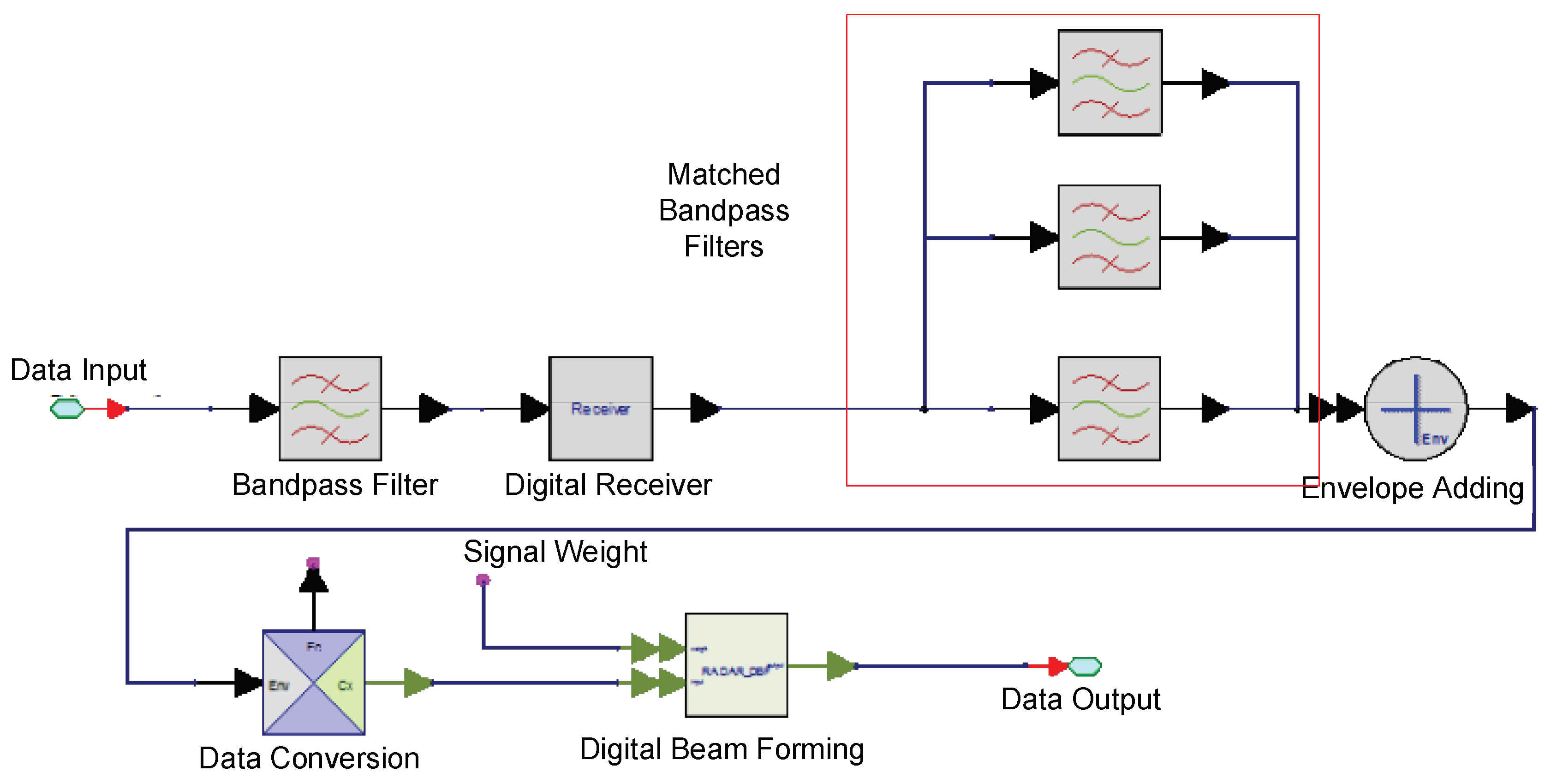
The data-receiving module is one of the most important modules in MIMO radar. Through this module, MIMO radar will receive the signal reflected by the radar target and calculate the radar targets such as speed, distance, DOA, and other information through the process of matching filtering, detection, and beam forming. The structure of the data-receiving module of traditional MIMO radar system is shown in
Figure 6.
In
Figure 6, three filters are listed as an example but, in an actual situation, the filters should be matched to the number of transmitter orthogonal signals, and the useful target information is filtered after the data-processing and digital beam-forming (DBF) processes. Assuming the MIMO radar can transmit
M orthogonal waveforms and each link needs corresponding matching filter, then the
M ×
N matching filters will make the system very complex and expensive for maintenance.
3.3. Signal Receiving and Processing Module
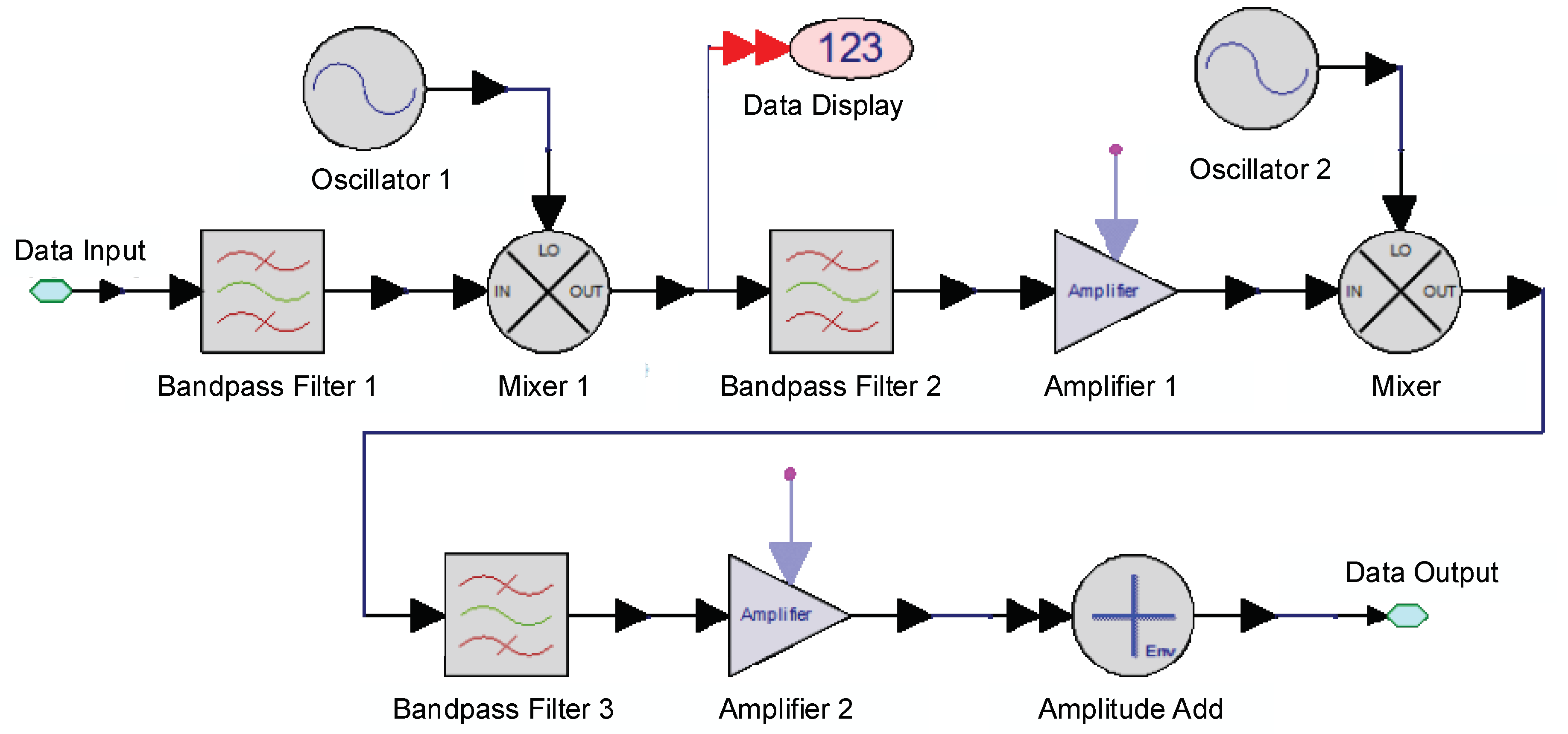
The signal receiving and processing module was mainly completed by a related algorithm in Matlab software. Firstly, the received signal needed to be down-converted from an RF signal to a baseband signal for analysis. In order to reduce the interference, two down-conversion processes were performed after the bandpass filters, which were used for filtering out other interferences introduced by the mixing. The CA-CFAR process eliminates the impact of false alarm probability and returns the target information. If the target is successfully detected, the return value is 1, otherwise it is 0. Finally, several repeated measurements were performed to obtain the average value of the target detection probability. The frequency conversion module is shown in
Figure 7.
The working flow of the frequency conversion module is as follows. The received signal went through two mixers to convert the signal to the middle frequency and the baseband frequency. After each frequency conversion, the signal passed through the bandpass filter to filter out the interference signal and was then rectified through a power amplifier. The final output signal will be analyzed in next step. The structure of the upper and lower frequency conversion modules is basically the same. Since the received echo signals are mixed with various noise and disturbances in the time domain, the target will not be observed directly. It is necessary to switch the time domain signals into frequency domain signals to filter the interference of time domain noise and clutter.
There are many kinds of system clutter, and the common probability density distributions include Weibull distribution, Rayleigh distribution, log–normal distribution, and
K distribution. The expression of the Rayleigh distribution and the
K distribution are shown in (18) and (4), respectively. The expressions for the Weibull distribution and the log–normal distribution are:
where
μ and
θ are the mean value and standard deviations of the normal distribution, respectively.
λ and
K are the scaling factor and the shape coefficient of Weibull distribution, respectively.
When the Doppler frequency is 100 Hz, the frequency of the clutter sources and the pulse repetition are 10 GHz and 1 kHz, respectively. The power spectral density (PSD) obeys the Gaussian distribution, and the sampling rate of the system is 10 MHz. The scale factor, shape coefficient, and the variance of K distribution are all 1.
The signal clutter is different for different power spectral densities. The general clutter power spectrum density includes Gaussian power spectrum, Cauchy power spectrum, all-pole power spectrum, and so on. In fact, the concept is generally used to measure the capacity of carrying the electromagnetic waves for every unit. In the dynamic target detection process, the Doppler shift of the received pulse radar signal can be obtained by FFT. Fd and fPRF are the target Doppler shift and pulse repetition rate of the pulse radar, respectively. N and n are the sampling number and the serial number of the FFT process, respectively.
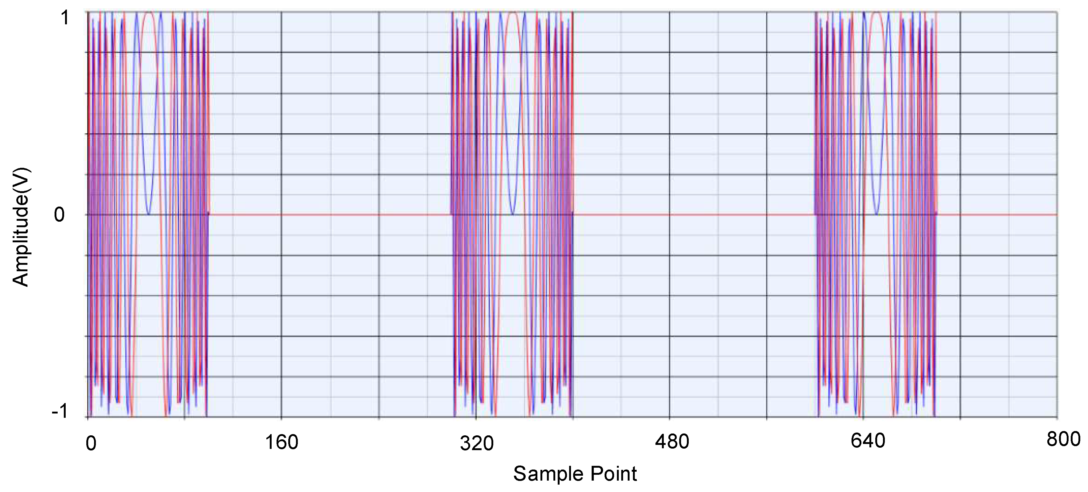
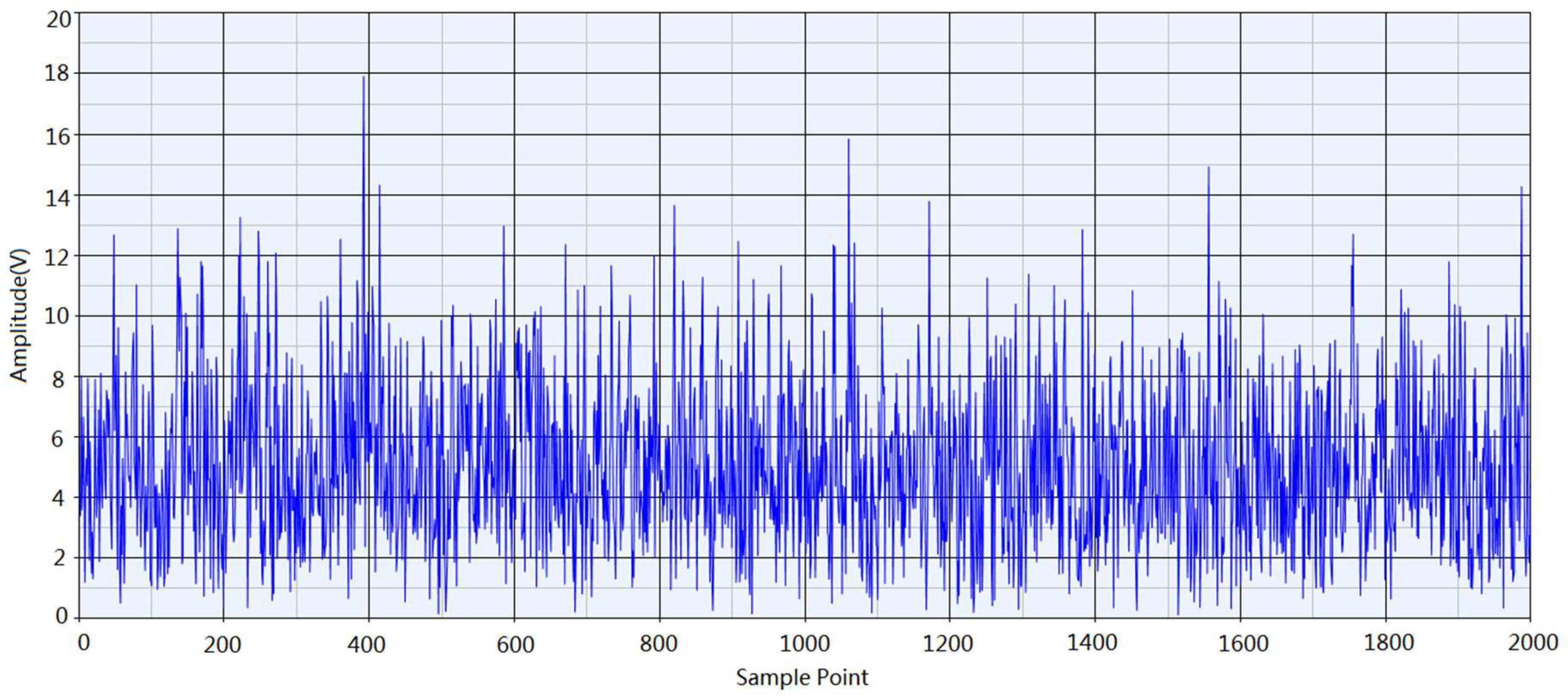
It can be seen from (21) that the number of FFT sampling points affects the system accuracy of the Doppler frequency shift. The calculation error will be reduced if the FFT number is large enough, thus the final solution of the Doppler frequency shift is more accurate, but the corresponding amount of calculation required will become larger. The number of points can be changed according to the requirements of parameter accuracy, and the number must be an integer power of 2. In order to balance the calculation and system accuracy, the number of FFT in this platform was 32 for the simulation. If the target was not detected, no significant peaks are found in the received waveform (
Figure 8). The distance between the target and the radar can be obtained by (22).
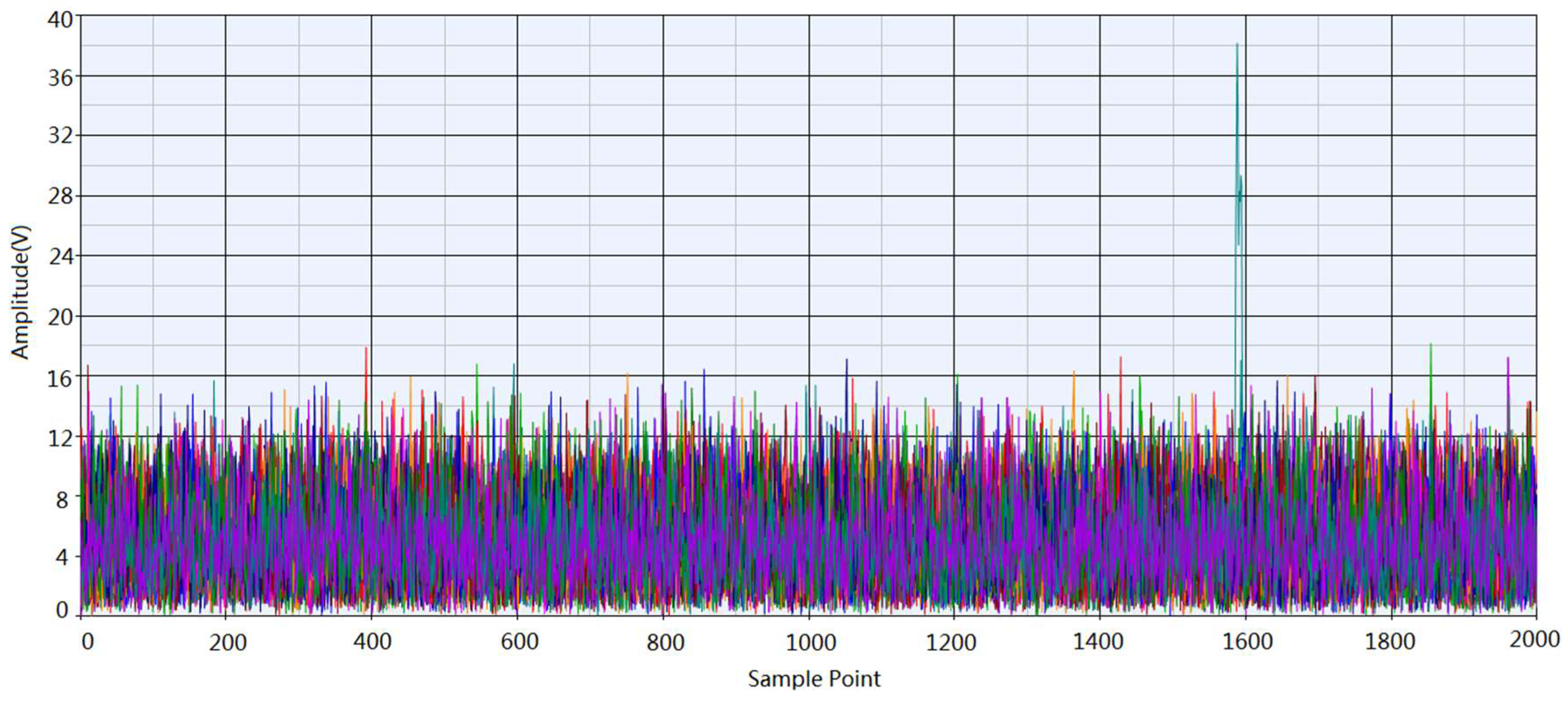
The Doppler frequency shift is also related to the pulse repetition frequency, which determines the upper limit that the system can measure. In different application situations, the pulse repetition frequency needs to be carefully selected to satisfy different target speeds. After the signal processing, if the target was detected, as is shown in
Figure 9, there is a peak in amplitude and its position corresponds to the horizontal coordinate of sampling points, which means the position of the target.
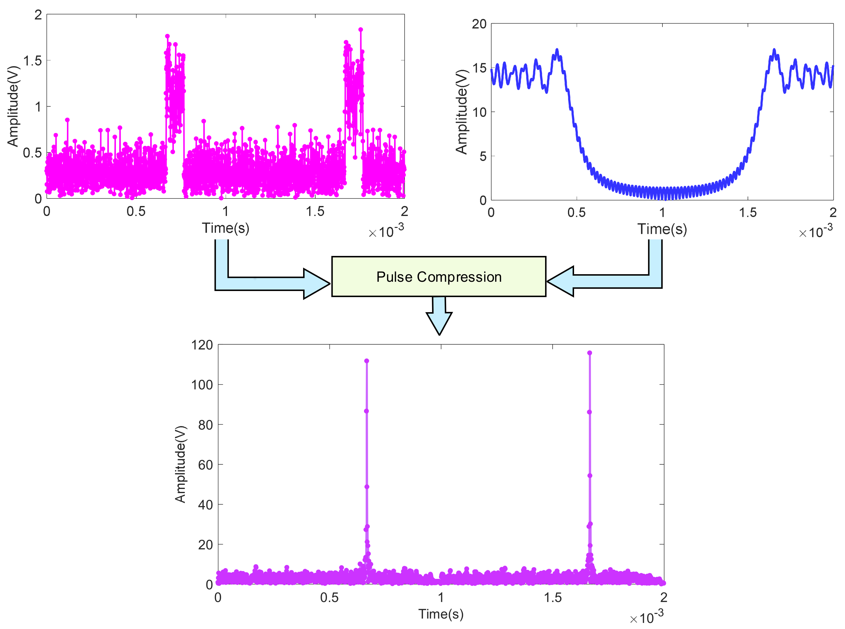
The blind speed phenomenon exists in the pulse radar mechanism. If the range is too small, the target may not be able to detect the result correctly when the target speed is greater. In order to solve this problem, pulse compression (PC) can be used to compress the received waveform into narrow pulses to improve the radar range resolution. In the simulation system, the problem can be solved by accessing a pulse compression element. The structure is shown in
Figure 10. This method can effectively improve the measurement performance of the MIMO radar.
It is worth noting that in the single RF link in MIMO radar systems, the two output signals are modulated by two sets of orthogonal bases, so the receiver also needs to establish a group of filters corresponding to the different orthogonal bases, which are controlled by SPDT switch. After the two groups of signals pass through different filters, we will obtain the speed and position information and the weighted average value as the final results. The traditional MIMO radar with the same 2 × 2 element structure cannot form groups of orthogonal bases even though there is no need for the switches, which has its own advantages and disadvantages. There is no doubt that, in the miniaturization of radar, single link RF MIMO radar is more suitable than traditional MIMO radar.
4. System Performance Discussion
In order to verify the correctness of the single RF link MIMO radar theory and its superiority compared to traditional MIMO radar, this section will compare the performance of target detection in the single RF link MIMO radar system and the traditional MIMO radar system under the ideal environment, which will focus on the speed and distance detection capability.
4.1. Performance Comparison Results
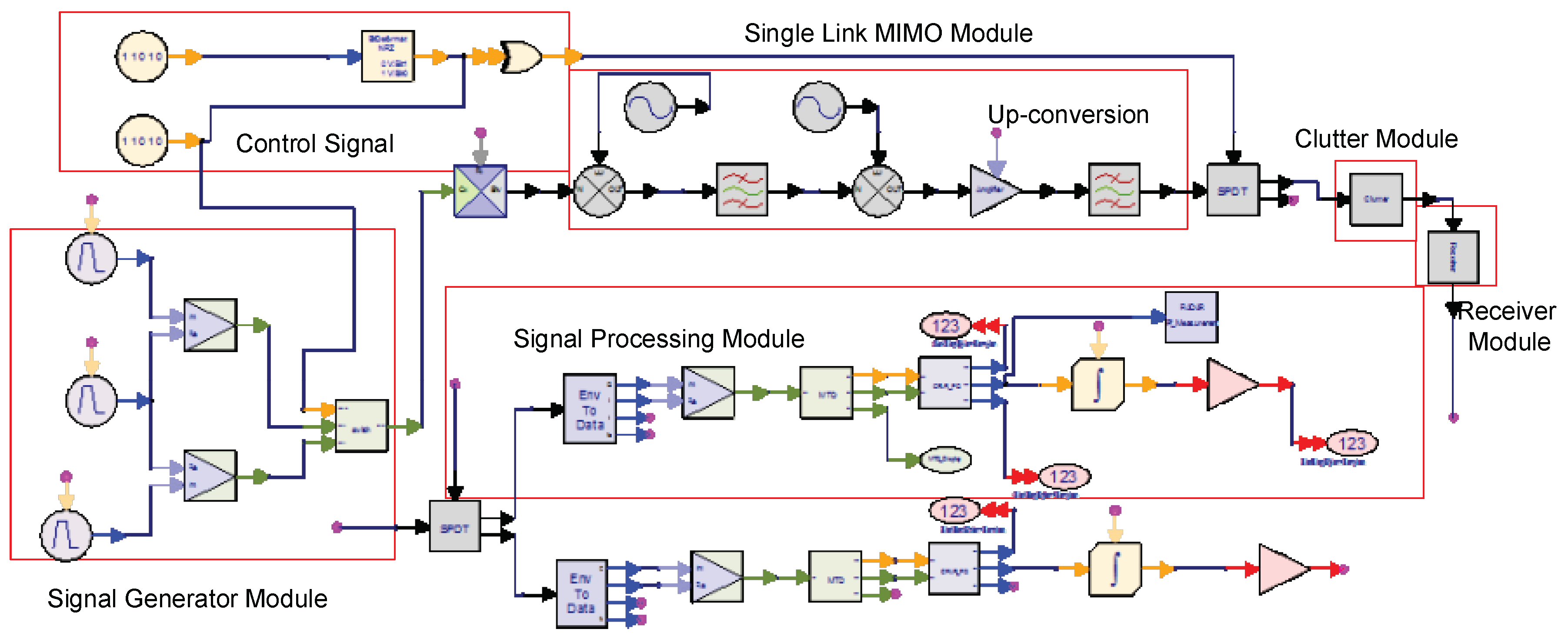
Unlike traditional MIMO radar, single link RF MIMO radar first generates control signals through two random digital signals. One of the signals is the control signal of the initial orthogonal basis, and the result of the two signal XOR operations controls the opening direction of the SPDT switch. In this work, two pseudorandom codes were used (PN15 and PN9).
The emission waveform is reflected by the radar target, which can be considered as the modulation process that carries the speed and distance information of the radar target on the transmitting waveform. The clutter interference in the channel adopts Rayleigh clutter, which is added to the transmitting signal by the clutter module. At the receiving end, the single link MIMO system can recover the two pre-modulated signals with a low bit-error rate. The restored signals will enter the correct matching filter. Then, we can filter out the unwanted clutter and noise in the reflected signal and get the velocity and distance information of the target through FFT. The CA-CFAR algorithm was adopted to get the result of the detected target. Finally, the Monte Carlo method was used to calculate the detection probability of the system.
The sampling frequency and the working frequency of the simulation were 20 MHz and 10 GHz, respectively. The baseband transmission with 60 MHz signal was up-converted to the middle frequency of 2.9 GHz. The repetition rate and the width of the pulse were 20 kHz and 500 ns, respectively. The simulation system setup in SystemVue software is shown in
Table 2.
As for the Swerling 0 target with radar distance of 9000 m and speed of 270 m/s, the target velocity and target distance of the two radar systems can be acquired from
Figure 11. The traditional MIMO radar system can be acquired by replacing the single-link MIMO module with the module shown in
Section 3. The results are compared in
Table 3 with the system setup shown in
Table 2.
It is not difficult to find that the ideal detection capability of target distance and velocity in single RF link MIMO radar and normal MIMO radar is basically the same. For both the detection of target velocity or the target distance, the error rate is kept in a small range with a slight difference, which is due to the calculation accuracy of the simulation platform. The detection speed of the two kinds of radars differ by only one sampling point, which can be seen as a calculation error and can be effectively reduced by increasing the number of FFT. In summary, the proposed single RF link MIMO radar can achieve the desired effect, as expected.
The detection probability of radar was measured by Monte Carlo method. D(t) is the indicating function that represents the result of target detection. If it equals 0, the target is not found, and 1 denotes that the target is detected. After 1000 simulations, the detection probability of single RF link MIMO radar and traditional MIMO radar were both above 99%, which verifies the correctness of the single RF link MIMO radar system.
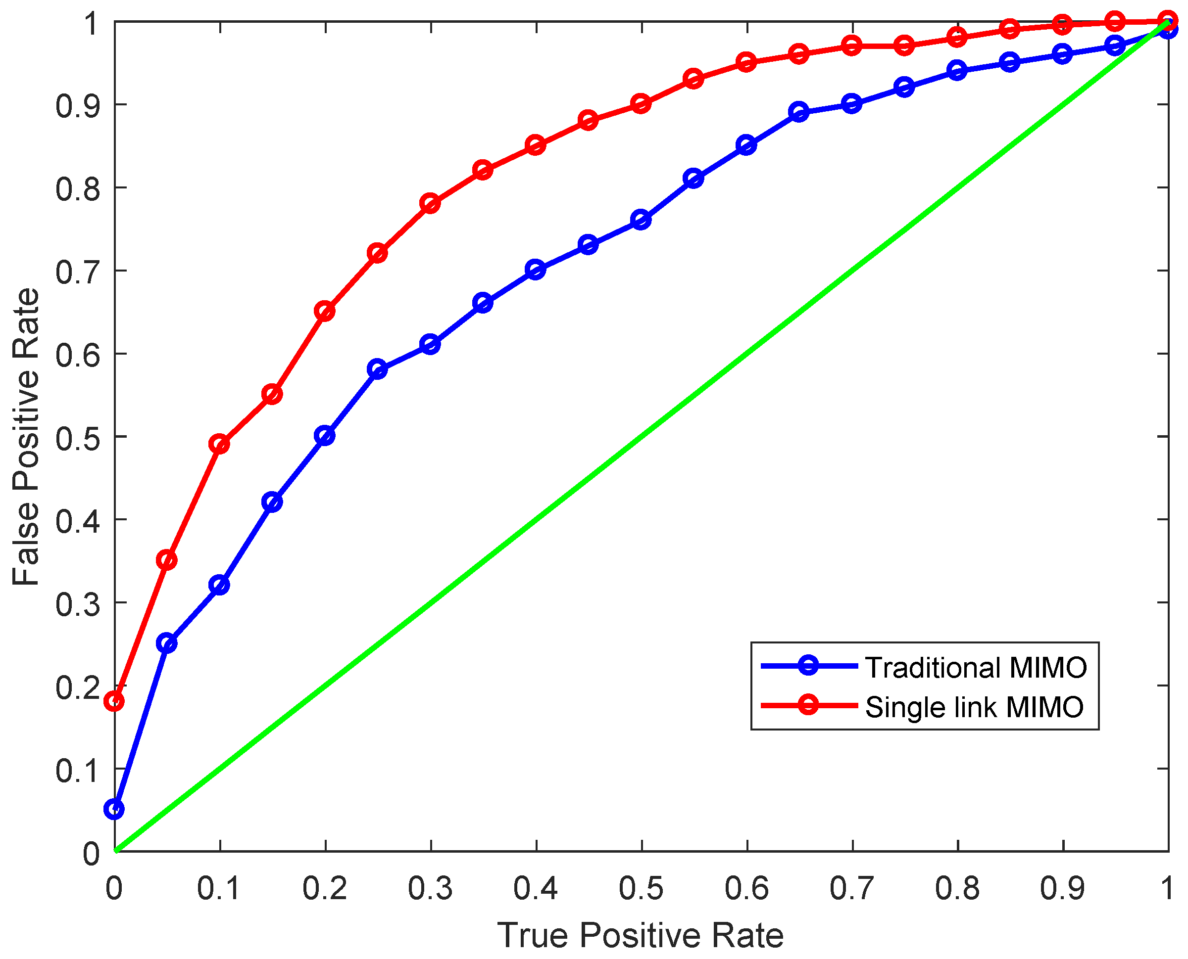
The receiver operating characteristic (ROC) curve, or the sensitivity curve, can be used to characterize the detection performance of MIMO radar [
38]. The working characteristic curve of the subjects is composed of false positive rate as the horizontal axis and true positive rate as the longitudinal axis. The true positive rate can also be denoted as the sensitivity, which means the accurate prediction probability for each radar signal of all enemy aircrafts. The true positive rate can also be called the specificity, which indicates the false prediction probability of each radar signal of all non-enemy aircrafts. Because each radar’s prediction standard varies, the sensitivity and specificity combinations are also different.
The more that the ROC curve is distributed toward the top left corner, the more accurate the detection system. The ROC curve closest to the upper left corner has the best threshold with the least error and the lowest total number of false positives and false negatives. The ROC curves of the two radar systems are drawn under the same coordinates to compare their performance, as is shown in
Figure 12. As can be concluded from the results, the single-link MIMO radar is nearer to the upper left corner than the traditional MIMO radar. The larger area under curve (AUC) indicates a better performance and higher accuracy of the single-link RF MIMO radar.
4.2. Parameter Discussion on System Performance
Compared with the traditional MIMO radar, single RF link MIMO radar has its disadvantages. For example, it uses too many SPDT switches, which will affect the overall detection probability of the system, such as the bit error rate of the control signal. Although the ideal single RF MIMO radar has excellent performance (although in nonideal circumstances), the switching time, isolation, switch loss, and other parameters of the SPDT switch will exert influence on the performance of single RF link MIMO radar to some extent, such as the radar dynamic range and the target detection probability.
This section is based on the radar simulation platform established in the
Section 3, and the theoretical analysis and simulation verification are discussed. Different parameters that influence the performance of the single RF link MIMO radar system are analyzed. For the simulation described in this paper, the initial simulation system parameter setup for single RF link MIMO radar is shown in
Table 4.
4.2.1. Switch Time
The switching time refers to the time consumed when the switch is changed from status 1 to state 2. For different conditions, Ton and Toff, can be used to indicate the starting point and ending point, respectively. For SPDT switches, the switching time is 0 under ideal conditions, and two-way signals can be seamlessly switched at any time. In the nonideal case, the signal is changing during the switching time, which will lead to the control signal error result during the sampling process. In order to eliminate the error of the control signal, Ton and Toff should be smaller than the sampling interval to ensure the correctness of the control signal. With a stable symbol rate, this goal is achieved by selecting switch components with appropriate switching time.
The switching process of the SPDT switch can be regarded as a linear change process in a very short time. Setting
v1(
t) as input signal and
v2(
t) as the control signal,
v3(
t) and
v4(
t) as two outputs, and the threshold value of control signal as 0.5, if
v2(
t) is larger than 0.5, the main input signal outputs from the
v3(
t) path. If the switch is switched at
t =
T instant, the two outputs are:
If
v2(
t) is smaller than 0.5, the main input signal outputs from the
v4(
t) path. If the switch is switched at
t =
T instant, the two outputs are:
It can be concluded that to prevent any error in the control signal, Ton or Toff should be less than the sampling time interval. In the case of fixed symbol rate, we want to achieve this goal by selecting components that have a suitable switching time.
4.2.2. Isolation
Isolation refers to the ratio of the power of the initial signal to the power of the other ports, the general unit is dB. It is an important indicator of the performance of the MIMO system, which can be described as:
Pi and Ps represent the power of the input port and the isolation port, respectively. Low isolation will lead to mutual confusion of signal components between two signals, causing erred judgement for the radar-receiving part. The ideal condition set in the simulation system is 200 dB. In actual engineering, the requirements depend on the specific circumstances. When 30 dB is used, the output signal of the isolated port is 0.1% of the output signal of the original port, which can meet engineering requirements in most cases.
From (26) and (27), we can infer that the antenna that is not occupied will transmit signals outward due to isolation. Because of the existence of this signal, the signal energy in the working link will be reduced and the performance of the system will be affected. Therefore, for the single RF link MIMO radar system, because of the multiple SPDT switches, the isolation index plays a more important role than other parameters. Theoretically, the higher the isolation degree, the greater the energy employed when the other conditions are constant. For the switches selected in this study, the isolation is different at various frequencies, with higher frequency responding to lower isolation. Although the specific isolation value is not given in the case of 10 GHz, the isolation degree under 27 GHz has sufficiently low isolation, which can be used in X band single RF link MIMO radar applications.
4.2.3. Signal-to-Noise Ratio
Signal-to-noise ratio (SNR) is an important indicator of performance for both MIMO radar and single RF link system. The SNR is the ratio of signal power to noise power in the channel:
For a single RF link communication system, SNR is positively correlated with channel capacity. In theory, when the SNR increases to a certain extent, its performance is the same as the traditional MIMO channel. For MIMO radar systems, targets with higher SNR are more likely to be detected. However, because of the introduction of the extra SPDT switch, the input two-tone third-order intercept point (IIP3) value of the switch will impose additional restrictions on the system performance. If it exceeds this limit, the switch will enter the nonlinear operating range during the receiver processing, resulting in the deviation of the result. Therefore, the SNR of single RF link MIMO radar system should be controlled in a certain range.
When the signal power is predetermined, the SNR of the system will decrease with the increase of clutter energy. Therefore, in order to explain their relationship, the remaining conditions were set as follows. The insertion loss and isolation were 0.5 dB and 30 dB, respectively. The clutter amplitudes ranged from 8 V to 14 V with a step length of 1 V, and Monte Carlo method was used for 1000 simulations. The noise amplitude and clutter power were positively correlated. The influence of the clutter amplitude on the detection probability of the single RF MIMO radar system is shown in
Table 5. When the clutter amplitude is smaller than 8 V, the detection probability of the target is higher than 99.8%, which is not listed in the table. From the data, we can conclude that the clutter amplitude has a great impact on the single RF link MIMO radar. The target detection probability decreases with increasing clutter amplitude and the speed of the detection probability reduction gradually accelerates. In this system, when the clutter amplitude is 11 V, the detection probability of the target begins to decrease greatly. When it reaches 14 V, the detection probability is reduced to the lowest value of 97.8% in the table.
When the SNR is low, the single RF link MIMO radar system discussed in this paper is still ideal, which means the signal can still be recovered completely. When the single link RF system is used in an actual situation, the signal cannot be correctly demodulated by the low SNR condition because the signal will not be correctly matched with the bandpass filter, thus the signal detection probability will be reduced. So, the SNR is more important for the single RF link MIMO radar system than for the traditional MIMO radar system.
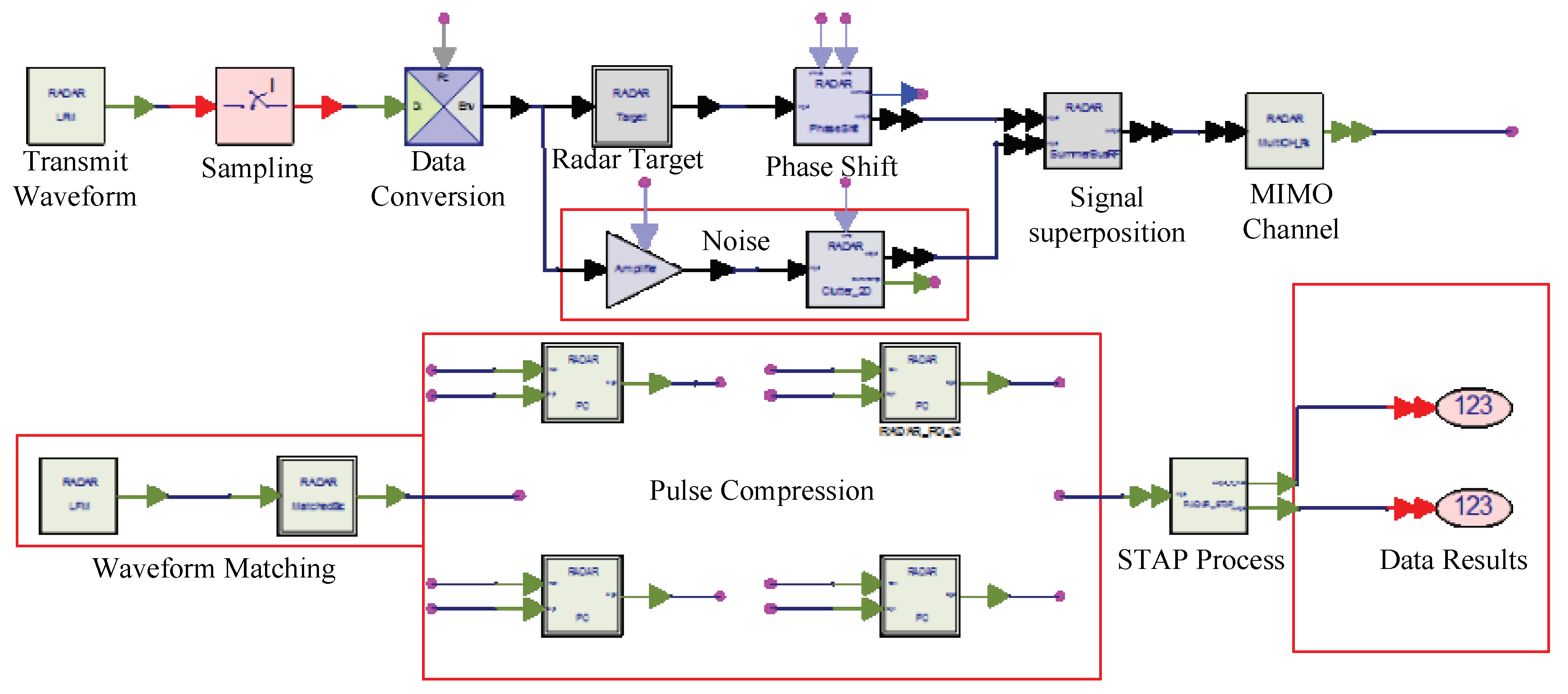
In this work, only one kind of clutter was studied, but in a real situation the radar system is often disturbed by many types of clutter. At this point, the system performance will inevitably be influenced. To solve this problem, we can add matching filters at the receiver part. If the actual clutter power or noise power has seriously affected the reception of the target—that is, the detection probability is lower than the allowed limit of the system—the space-time adaptive processing (STAP) can be used to suppress the clutter and noise of the received signal. The schematic diagram of the STAP process carried out by conventional radar is shown in
Figure 13.
The transmitting signal passes through the radar target module and the radar shift module, which inserts the continuous changing phase in the time interval, while the other branch produces clutter interference. The two signals are superimposed in the time domain and transmitted through the MIMO channel. The whole system is made up of four antennas and the four channel signals are processed by the pulse-compressed modules. Finally, the results are obtained through the STAP element.
4.2.4. Insertion Loss
Insertion loss is also an important character of RF devices. If the insertion loss is too large, the error rate will be high and deteriorate system performance. The insertion loss can be expressed as:
To explore the effect of insertion loss for single RF link MIMO radar system, the SPDT switch insertion loss ranging from 0 dB to 3 dB with scanning interval of 0.5 dB was investigated. The single RF link MIMO radar system detection probability values that varied with the insertion loss are listed in
Table 6, which were obtained from the 1000 simulations performed by Monte Carlo method.
It can be concluded that the high insertion loss will result in lower target detection probability. When the insertion loss is less than 1.5 dB, the detection probability can reach more than 99%. With the increase in the insertion loss, the detection probability will decrease rapidly, which is almost below 98% when the insertion loss is higher than 2.5 dB. This is because the insertion loss will cause energy loss at the transmitter antenna, which weakens the receiving signal.
4.2.5. Dynamic Range
The introduction of insertion loss will also affect another important performance index of the radar system, the dynamic range. Within this range, the radar receiver will not be distorted due to the excessive amplitude of the received signal or not be detected because the receiving signal is too small.
Pmax and Pmin are the upper limit and lower limit of the receiving signal amplitude, respectively. In order to make sure the system is working under the linear area of the receiver, the transmitter has to consume more energy, which reduces the efficiency of the single RF link MIMO radar system. Meanwhile, the introduction of insertion loss will theoretically increase and lead to the decrease of dynamic range. Therefore, for the single RF link MIMO radar, the insertion loss introduced by the newly added SPDT switch will greatly affect the performance of the radar. In order to work properly, it is very important to adopt an SPDT switch with small loss.
In order to reduce the impact of insertion loss, it is necessary to first detect the normal working state of each part of the system to prevent unnecessary loss due to the internal problems of the system. Secondly, the elements with low insertion loss can be selected. If the switch is not available, the gain of the transmitter amplifier can be properly increased to a certain range to compensate for the loss of the signal energy caused by the insertion loss. In this system, the gain of the transmitter amplifier is 10. In order to explore the influence of amplifier gain on the detection probability of the target, the initial insertion loss was set to 3 dB to make the results more obvious. Under the conditions listed in
Table 3, 1000 groups of experiments for each gain were carried out to get the detection probability, as is shown in
Figure 14.
From this result, we can see that detection probability increases with the increase of transmitter amplifier gain. When the power amplifier multiplier is 11.5, the detection probability has risen from the lowest value of 96.8% to 99.5%. When the power amplifier multiple is 13, the detection probability is very close to 1. The result indicates that it is feasible to compensate for the insertion loss introduced by the new SPDT switch by improving the gain of the power amplifier at the transmitter side. The physical properties, such as power and capacity of switches and other components, have not been taken into consideration. Under the actual working conditions of radar, the choice of power amplifier needs to be varied according to the performance of internal physical components.
To sum up, in order to achieve higher performance of the single RF link MIMO radar system, the switching time, isolation, and insertion loss of the insertion switch should meet the requirements of the real condition. In theory, if we choose an SPDT switch with excellent performance, we can solve the above problems. Some parameters can be corrected according to the relationship between the performance and parameters of the MIMO radar and the precision of the radar system.


