Degree Approximation-Based Fuzzy Partitioning Algorithm and Applications in Wheat Production Prediction

Abstract
1. Introduction
2. Related Works
2.1. Literature Review
2.2. Mathematical Preliminary
3. The Proposed Framework
3.1. The Need of This Framework
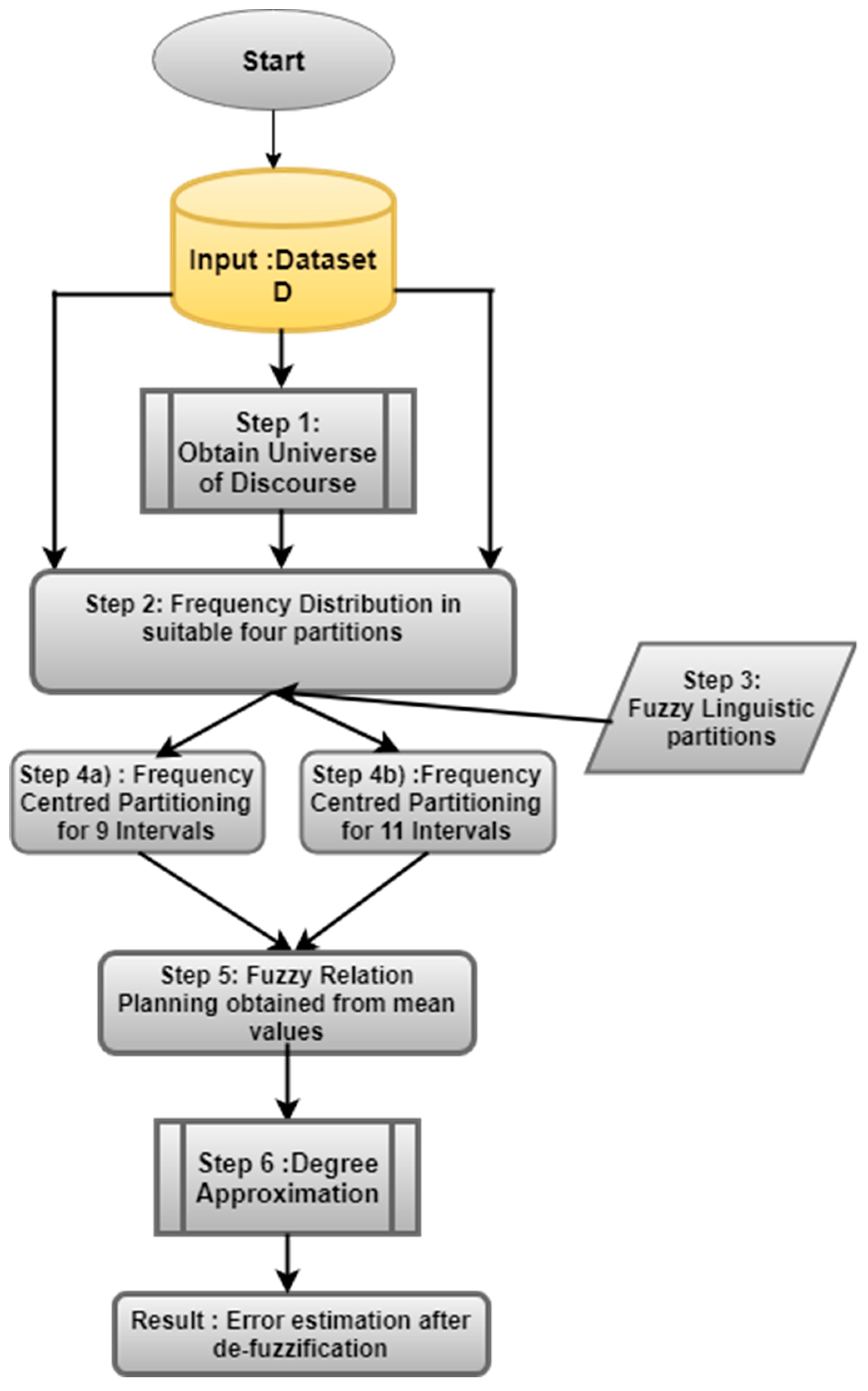
3.2. The Workflow Diagram
3.3. DAbFP Algorithm
3.4. Numerical Example
4. Results and Discussion
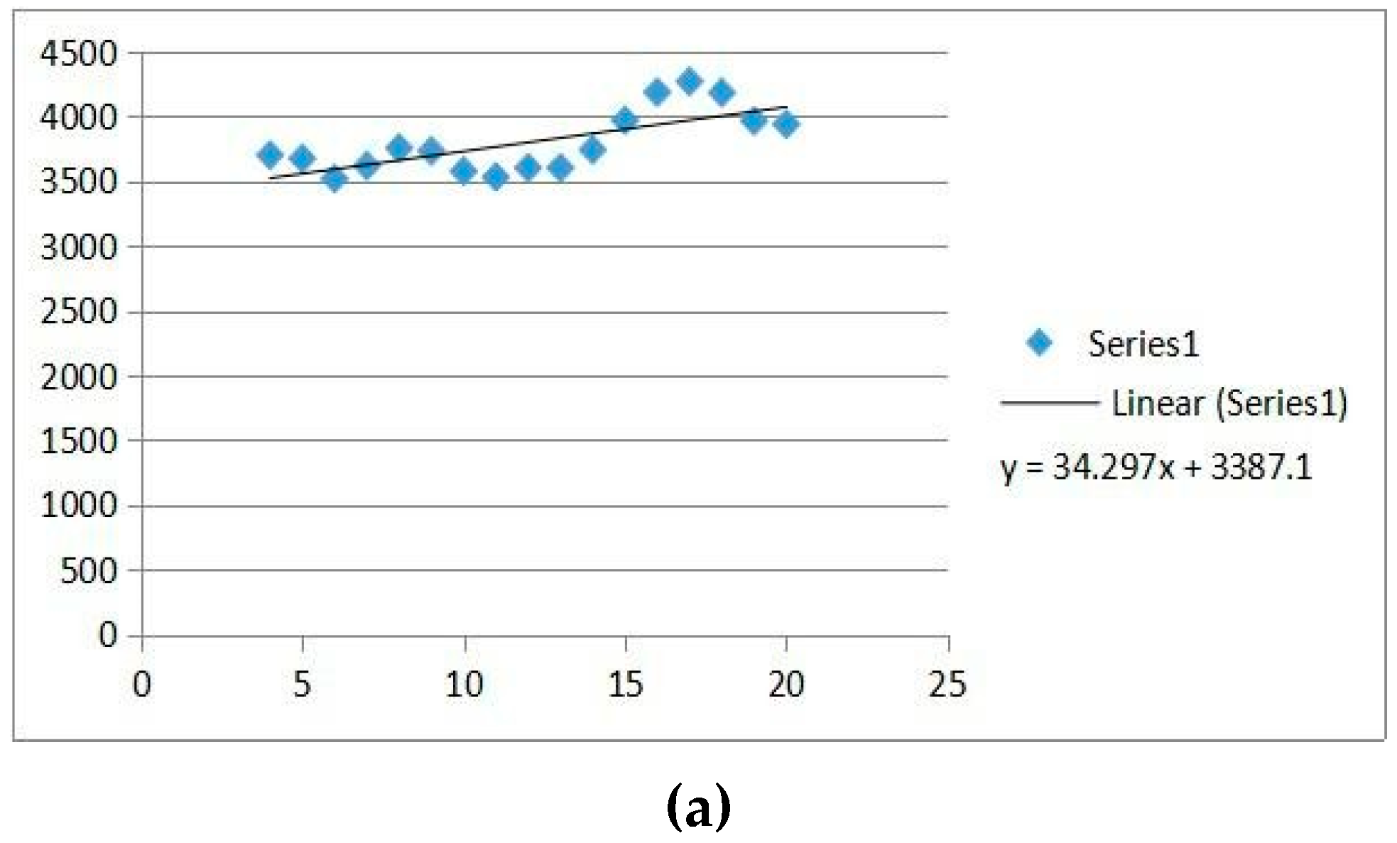
4.1. Linear Polynomial
4.2. Quadratic Polynomial
4.3. Cubic Polynomial
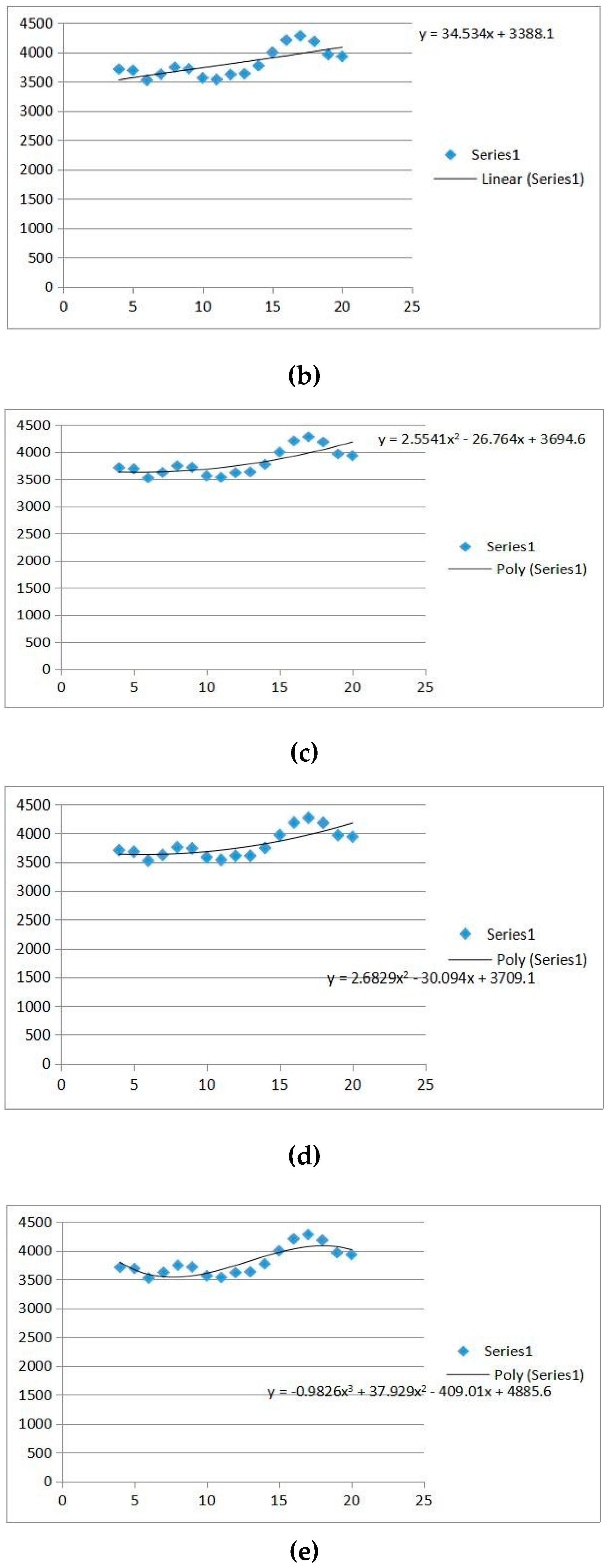
4.4. Results
5. Conclusions
Author Contributions
Funding
Conflicts of Interest
Compliance with Ethical Standards
References
- Song, Q.; Chissom, B. Fuzzy time series and its models. Fuzzy Sets Syst. 1993, 54, 269–277. [Google Scholar] [CrossRef]
- Song, Q.; Chissom, B. Forecasting enrollments with fuzzy time series-Part, I. Fuzzy Sets Syst. 1993, 45, 1–10. [Google Scholar] [CrossRef]
- Song, Q.; Chissom, B. Forecasting enrollments with fuzzy time series-Part II. Fuzzy Sets Syst. 1994, 62, 1–8. [Google Scholar] [CrossRef]
- Song, Q.; Leland, R.; Chissom, B. A new fuzzy time-series model of fuzzy number observations. Fuzzy Sets Syst. 1995, 73, 341–348. [Google Scholar] [CrossRef]
- Choudhury, A.; Jones, J. Crop Yield Prediction Using Time Series Models. J. Econ. Econ. Educ. Res. 2014, 15, 53. [Google Scholar]
- Kumar, S.; Kumar, N. A Novel Method for Rice Production Forecasting Using Fuzzy Time Series. Int. J. Comput. Sci. Issues 2012, 9, 455. [Google Scholar]
- Kumar, S.; Kumar, N. Two Factor Fuzzy Time Series Model for Rice Forecasting. Int. J. Comput. Math. Sci. 2015, 4, 2347–8527. [Google Scholar]
- Kumar, N.; Ahuja, S.; Kumar, V.; Kumar, A. Fuzzy time series forecasting of wheat production. Int. J. Comput. Sci. Eng. 2010, 2, 635–640. [Google Scholar]
- Egrioglu, E.; Aladag, C.; Yolcu, U.; Uslu, V.; Basaran, M. Finding an optimal interval length in high order fuzzy time series. Expert Syst. Appl. 2010, 37, 5052–5055. [Google Scholar] [CrossRef]
- Eğrioğlu, E. A New Time-Invariant Fuzzy Time Series Forecasting Method Based on Genetic Algorithm. Adv. Fuzzy Syst. 2012, 2012, 2. [Google Scholar] [CrossRef]
- Qiu, W.; Liu, X.; Li, H. A generalized method for forecasting based on fuzzy time series. Expert Syst. Appl. 2011, 38, 10446–10453. [Google Scholar] [CrossRef]
- Song, Q. A note on fuzzy time series model selection with sample autocorrelation functions. Cybern. Syst. 2003, 34, 93–107. [Google Scholar] [CrossRef]
- Garg, B.; Beg, M.; Ansari, A. Fuzzy time series model to forecast rice production. In Proceedings of the IEEE International Conference on Fuzzy Systems, Hyderabad, India, 7–10 July 2013. [Google Scholar]
- Huarng, K. Effective lengths of intervals to improve forecasting in fuzzy time series. Fuzzy Sets Syst. 2001, 123, 387–394. [Google Scholar] [CrossRef]
- Huarng, K. Heuristic models of fuzzy time series for forecasting. Fuzzy Sets Syst. 2001, 123, 369–386. [Google Scholar] [CrossRef]
- Hwang, J.; Chen, S.; Lee, C. Handling Forecasting Problems using Fuzzy Time Series. Fuzzy Sets Syst. 1998, 100, 217–228. [Google Scholar] [CrossRef]
- Lee, L.; Wang, L.; Chen, S. Handling Forecasting Problems based on Two-Factors High-Order Time Series. IEEE Trans. Fuzzy Syst. 2006, 14, 468–477. [Google Scholar] [CrossRef]
- Sheta, A. Software Effort Estimation and Stock Market Prediction Using Takagi-Sugeno Fuzzy Models. In Proceedings of the IEEE International Conference on Fuzzy System, Vancouver, BC, Canada, 16–21 July 2006; pp. 171–178. [Google Scholar]
- Chu, S.; Kim, H. Automatic knowledge generation from the stock market data. In Proceedings of the 93 Korea Japan Joint Conference on Expert Systems, Seoul, South Korea, 1993; pp. 193–208. [Google Scholar]
- Wolfers, J.; Zitzewitz, E. Prediction markets in theory and practice. Natl. Bureau Econ. Res. 2006, 1–11. [Google Scholar] [CrossRef]
- Hammouda, K.; Karray, F. A Comparative Study of Data Clustering Techniques. Available online: www.pami.uwaterloo.ca/pub/hammouda/sde625-paper.pdf (accessed on 10 November 2018).
- Babuska, R.; Roubos, J.; Verbruggen, H. Identification of MIMO systems by input-output TS fuzzy models. In Proceedings of the Fuzzy-IEEE’98, Anchorage, AK, USA, 4–9 May 1998. [Google Scholar]
- Van Eyden, R.J. Application of Neural Networks in the Forecasting of Share Prices; Finance and Technology Publishing: Haymarket, VA, USA, 1996. [Google Scholar]
- Hiemstra, Y. A stock market forecasting support system based on fuzzy logic. In Proceedings of the Twenty-Seventh Hawaii International Conference on System Sciences HICSS-94, Wailea, HI, USA, 4–7 January 1994. [Google Scholar]
- Chiu, S. Fuzzy model identification based on cluster estimation. J. Intell. Fuzzy Syst. 1994, 2, 267–278. [Google Scholar]
- Gomide, F. A review of: Fuzzy Sets and Fuzzy Logic: Theory and Applications by George Klir and Bo Yuan, Prentice Hall PTR. Int. J. Gen. Syst. 1997, 26, 292–294. [Google Scholar] [CrossRef]
- Ribeiro, R.; Hans-Jürgen, Z.; Yager, R.; Kacprzyk, J. Soft Computing in Financial Engineering; Physica: Heidelberg, Germany, 1999. [Google Scholar]
- Dostál, P. The Use of Optimization Methods in Business and Public Services. In Handbook of Optimization Intelligent Systems Reference Library; Springer: Berlin/Heidelberg, Germany, 2013; pp. 717–777. [Google Scholar]
- Dostál, P. The Use of Soft Computing for Optimization in Business, Economics, and Finance. In Meta-Heuristics Optimization Algorithms in Engineering, Business, Economics, and Finance; IGI Global: Hershey, PA, USA, 2013; pp. 41–86. [Google Scholar]
- Li, Z.; Chen, G.; Halang, W. Anticontrol of Chaos for Takagi-Sugeno Fuzzy Systems, Integration of Fuzzy Logic and Chaos Theory; Springer: Berlin/Heidelberg, Germany, 2006; pp. 185–227. [Google Scholar]
- Peters, E.E. Fractal Market Analysis: Applying Chaos Theory to Investment and Economics; Wiley: New York, NY, USA, 2009. [Google Scholar]
- Peters, E.E. Chaos and Order in the Capital Markets: A New View of Cycles, Prices, and Market Volatility; John Wiley & Sons: New York, NY, USA, 1996. [Google Scholar]
- Trippi, R.R. Chaos & Nonlinear Dynamics in the Financial Markets; Irwin Professional Publishing: Cheney, KS, USA, 1995. [Google Scholar]
- Altrock, C. Fuzzy Logic & Neurofuzzy—Applications in Business & Finance; Prentice Hall: Upper Saddle River, NJ, USA, 1996. [Google Scholar]
- Hamam, A.; Eid, M.; El Saddik, A.; Georganas, N.D. Fuzzy logic system for evaluating Quality of Experience of haptic-based applications. In International Conference on Human Haptic Sensing and Touch Enabled Computer Applications; Springer: Berlin/Heidelberg, Germany, 2008; pp. 129–138. [Google Scholar]
- Alreshoodi, M.; Woods, J. An Empirical Study based on a Fuzzy Logic System to Assess the QoS/QoE Correlation for Layered Video Streaming. In Proceedings of the IEEE International Conference on Computational Intelligence and Virtual Environments for Measurement Systems and Applications, Milan, Italy, 15–17 July 2013. [Google Scholar]
- Doctor, F.; Hagras, H.; Callaghan, V. A Fuzzy Embedded Agent based Approach for Realizing Ambient Intelligence in Intelligent Inhabited Environments. Ph.D. Thesis, The University of Texas at Arlington, Arlington, TX, USA, 2005. [Google Scholar]
- Wang, L.X.; Mendel, J.M. Generating fuzzy rules by learning from examples. IEEE Trans. Syst. Man Cybern. 1992, 22, 1414–1427. [Google Scholar] [CrossRef]
- Castillo, O.; Melin, P. A new approach for plant monitoring using type-2 fuzzy logic and fractal theory. Int. J. Gen. Syst. 2004, 33, 305–319. [Google Scholar] [CrossRef]
- Yolcu, U.; Egrioglu, E.; Uslu, R.V.R.; Basaran, M.A.; Aladag, C.H. A new approach for determining the length of intervals for fuzzy time series. Appl. Soft Comput. 2009, 9, 647–651. [Google Scholar] [CrossRef]
- Garg, B.; Beg, M.M.S.; Ansari, A.Q.; Imran, B.M. Fuzzy Time Series Prediction Model, Communications in Computer and Information Science; Springer: Berlin/Heidelberg, Germany, 2011; Volume 141, pp. 126–137. [Google Scholar]
- Garg, B.; Beg, M.M.S.; Ansari, A.Q.; Imran, B.M. Soft Computing Model to Predict Average Length of Stay of Patient, Communications in Computer and Information Science; Springer: Berlin/Heidelberg, Germany, 2011; Volume 141, pp. 221–232. [Google Scholar]
- Khuong, M.N.; Tuan, T.M. A New Neuro-Fuzzy Inference System for Insurance Forecasting. In Advances in Information and Communication Technology; Springer: Thai Nguyen, Vietnam, 2016. [Google Scholar]
- Son, L.; Thong, P. Some novel hybrid forecast methods based on picture fuzzy clustering for weather nowcasting from satellite image sequences. Appl. Intell. 2017, 46, 1–15. [Google Scholar] [CrossRef]
- Stathakis, D.; Savin, I.; Nègre, T. Neuro-fuzzy modeling for crop yield prediction. The International Archives of the Photogrammetry. Remote Sens. Spat. Inf. Sci. 2006, 34, 1–4. [Google Scholar]
- Lee, M.H.; Sadaei, J.H. Introducing polynomial fuzzy time series. J. Intell. Fuzzy Syst. 2013, 25, 117–128. [Google Scholar]
- Jilani, T.A.; Burney, S.M.A.; Ardil, C. Multivariate high order fuzzy time series forecasting for car road accidents. Int. J. Comput. Intell. 2007, 4, 15–20. [Google Scholar]
- Chen, S.M.; Hwang, J.R. Temperature prediction using fuzzy time series. IEEE Trans. Syst. Man Cybern. Part B Cybern. 2000, 30, 263–275. [Google Scholar] [CrossRef] [PubMed]
- Poulsen, J.R. Fuzzy Time Series Forecasting; Aalborg University Esbjerg: Esbjerg, Denmark, 2009. [Google Scholar]
- Detyniecki, M.; Bouchon-meunier, D.B.; Yager, D.R.; Prade, R.H. Mathematical Aggregation Operators and their application to video querying. Available online: http://citeseerx.ist.psu.edu/viewdoc/summary?doi=10.1.1.21.17 (accessed on 10 November 2018).
- Yalaz, S.; Arife, A. Fuzzy Linear Regression for the Time Series Data which is Fuzzified with SMRGT Method. Süleyman Demirel Üniversitesi Fen Bilimleri Enstitüsü Dergisi 2016, 20, 405–413. [Google Scholar] [CrossRef]
- Pant Nagar farm, G.B. Pant University of Agriculture and Technology, India. Available online: http://www.gbpuat.ac.in/facility/farm/index.html (accessed on 10 November 2018).
- Khan, M.; Son, L.; Ali, M.; Chau, H.; Na, N.; Smarandache, F. Systematic review of decision making algorithms in extended neutrosophic sets. Symmetry 2018, 10, 314. [Google Scholar] [CrossRef]
- Khoshnevisan, B.; Rafiee, S.; Mahmoud, O.; Mousazadeh, H. Development of an intelligent system based on ANFIS for predicting wheat grain yield on the basis of energy inputs. Inf. Process. Agric. 2014, 1, 14–22. [Google Scholar] [CrossRef]
- Kamali, H.; Shahnazari-Shahrezaei, P.; Kazemipoor, H. Two new time-variant methods for fuzzy time series forecasting. J. Intell. Fuzzy Syst. 2013, 24, 733–741. [Google Scholar]
- Yang, W.; Li, M.; Zheng, L.; Sun, H. Evaluation Model of Winter Wheat Yield Based on Soil Properties. In International Conference on Computer and Computing Technologies in Agriculture; Springer: Cham, Switzerland, 2015; pp. 638–645. [Google Scholar]
- Luna, I.; Ballini, R. Adaptive fuzzy system to forecast financial time series volatility. J. Intell. Fuzzy Syst. 2012, 23, 27–38. [Google Scholar]
- Kasabov, N.K.; Song, Q. DENFIS: Dynamic evolving neural-fuzzy inference system and its application for time-series prediction. IEEE Trans. Fuzzy Syst. 2000, 10, 144–154. [Google Scholar] [CrossRef]
- Aladag, C.; Egrioglu, E.; Yolcu, U.; Uslu, V. A high order seasonal fuzzy time series model and application to international tourism demand of Turkey. J. Intell. Fuzzy Syst. 2014, 26, 295–302. [Google Scholar]
- Pham, B.T.; Son, L.H.; Hoang, T.-A.; Nguyen, D.-M.; Bui, D.T. Prediction of shear strength of soft soil using machine learning methods. Catena 2018, 166, 181–191. [Google Scholar] [CrossRef]
- Son, L.; Huy, N.Q.; Thong, T.N.; Dung, T.T.K. An effective solution for sustainable use and management of natural resources through webGIS open sources and decision-making support tools. In Proceedings of the 5th International Conference on GeoInformatics for Spatial-Infrastructure Development in Earth and Allied Sciences, Hanoi, Vietnam, 9–11 December 2010. [Google Scholar]
- Tuan, T.; Chuan, P.; Ali, M.; Ngan, T.; Mittal, M.; Son, L. Fuzzy and neutrosophic modeling for link prediction in social networks. Evol. Syst. 2018, 1–6. [Google Scholar] [CrossRef]
- Kadir, M.K.A.; Ayob, M.Z.; Miniappan, N. Wheat yield prediction: Artificial neural network based approach. In Proceedings of the 4th International Conference on Engineering Technology and Technopreneuship (ICE2T), Kuala Lumpur, Malaysia, 27–29 August 2014. [Google Scholar]
- Vovan, T. An improved fuzzy time series forecasting model using variations of data. Fuzzy Optim. Decis. Mak. 2018, 1–23. [Google Scholar] [CrossRef]
- Georgi, C.; Spengler, D.; Itzerott, S.; Kleinschmit, B. Automatic delineation algorithm for site-specific management zones based on satellite remote sensing data. Precis. Agric. 2018, 19, 684–707. [Google Scholar] [CrossRef]
- Paustian, M.; Theuvsen, L. Adoption of precision agriculture technologies by German crop farmers. Precis. Agric. 2017, 18, 701–716. [Google Scholar] [CrossRef]
- Novak, V. Detection of Structural Breaks in Time Series Using Fuzzy Techniques. Int. J. Fuzzy Logic Intell. Syst. 2018, 18, 1–12. [Google Scholar] [CrossRef]
- Grzegorzewski, P. On Separability of Fuzzy Relations. Int. J. Fuzzy Logic Intell. Syst. 2017, 17, 137–144. [Google Scholar] [CrossRef]
- Phuong, P.T.M.; Thong, P.H.; Son, L.H. Theoretical Analysis of Picture Fuzzy Clustering: Convergence and Property. J. Comput. Sci. Cybern. 2018, 1, 17–32. [Google Scholar] [CrossRef]
- Jha, S.; Kumar, R.; Chatterjee, J.M.; Khari, M.; Yadav, N.; Smarandache, F. Neutrosophic soft set decision making for stock trending analysis. Evol. Syst. 2018, 1–7. [Google Scholar] [CrossRef]
- Ngan, R.T.; Son, L.H.; Cuong, B.C.; Ali, M. H-max distance measure of intuitionistic fuzzy sets in decision making. Appl. Soft Comput. 2018, 69, 393–425. [Google Scholar] [CrossRef]
- Giap, C.N.; Son, L.H.; Chiclana, F. Dynamic structural neural network. J. Intell. Fuzzy Syst. 2018, 34, 2479–2490. [Google Scholar] [CrossRef]
- Ali, M.; Son, L.H.; Thanh, N.D.; Van Minh, N. A neutrosophic recommender system for medical diagnosis based on algebraic neutrosophic measures. Appl. Soft Comput. 2018, 71, 1054–1071. [Google Scholar] [CrossRef]
- Ali, M.; Son, L.H.; Khan, M.; Tung, N.T. Segmentation of dental X-ray images in medical imaging using neutrosophic orthogonal matrices. Expert Syst. Appl. 2018, 91, 434–441. [Google Scholar] [CrossRef]
- Ali, M.; Dat, L.Q.; Son, L.H.; Smarandache, F. Interval complex neutrosophic set: Formulation and applications in decision-making. Int. J. Fuzzy Syst. 2018, 20, 986–999. [Google Scholar] [CrossRef]
- Son, L.H.; Tuan, T.M.; Fujita, H.; Dey, N.; Ashour, A.S.; Ngoc, V.T.N.; Chu, D.T. Dental diagnosis from X-Ray images: An expert system based on fuzzy computing. Biomed. Signal Process. Control 2018, 39, 64–73. [Google Scholar] [CrossRef]
- Nguyen, G.N.; Son, L.H.; Ashour, A.S.; Dey, N. A survey of the state-of-the-arts on neutrosophic sets in biomedical diagnoses. Int. J. Mach. Learn. Cybern. 2017, 1–13. [Google Scholar] [CrossRef]
- Ngan, R.T.; Ali, M.; Son, L.H. δ-equality of intuitionistic fuzzy sets: A new proximity measure and applications in medical diagnosis. Appl. Intell. 2018, 48, 499–525. [Google Scholar] [CrossRef]
- Ali, M.; Son, L.H.; Deli, I.; Tien, N.D. Bipolar neutrosophic soft sets and applications in decision making. J. Intell. Fuzzy Syst. 2017, 33, 4077–4087. [Google Scholar] [CrossRef]
- Thanh, N.D.; Ali, M.; Son, L.H. A novel clustering algorithm in a neutrosophic recommender system for medical diagnosis. Cognit. Comput. 2017, 9, 526–544. [Google Scholar] [CrossRef]
- Son, L.H.; Viet, P.V.; Hai, P.V. Picture inference system: A new fuzzy inference system on picture fuzzy set. Appl. Intell. 2017, 46, 652–669. [Google Scholar] [CrossRef]
- Son, L.H.; Tien, N.D. Tune up fuzzy C-means for big data: Some novel hybrid clustering algorithms based on initial selection and incremental clustering. Int. J. Fuzzy Syst. 2017, 19, 1585–1602. [Google Scholar] [CrossRef]


| F1 | very meagre produce |
| F2 | meagre produce |
| F3 | better than poor produce |
| F4 | not so quality produce |
| F5 | average production |
| F6 | superior produce |
| F7 | very superior produce |
| F8 | Very very superior produce |
| F9 | tremendous produce |
| Fuzzy Sets | Upper | Lower | Frequency |
|---|---|---|---|
| F1 | 233,200 | 343,355 | 3 |
| F2 | 233,355 | 343,511 | 2 |
| F3 | 233,511 | 343,666 | 2 |
| F4 | 233,666 | 343,822 | 3 |
| F5 | 233,822 | 344,133 | 4 |
| F7 | 234,133 | 344,288 | 3 |
| F8 | 234,288 | 344,444 | 2 |
| F9 | 234,444 | 344,600 | 1 |
| Fuzzy Sets | Upper | Lower | New Fuzzy Sets |
|---|---|---|---|
| AF1A | 932,007 | 3252.76 | Z1 |
| 3253.76 | 3303.8 | Z2 | |
| 3303.8 | 3356.66 | Z3 | |
| AF2A | 3356.66 | 3432.435 | Z4 |
| 3432.435 | 3512.2 | Z5 | |
| AF3A | 3512.2 | 3589.985 | Z6 |
| 3589.985 | 3677.75 | Z7 | |
| AF4A | 3677.75 | 3729.5 | Z8 |
| 3729.5 | 3771.45 | Z9 | |
| 3771.45 | 3823.3 | Z10 | |
| AF5A | 3823.3 | 3862.1985 | Z11 |
| 3862.1985 | 3900.175 | Z12 | |
| 3900.175 | 3949.9725 | Z13 | |
| 3949.9725 | 3988.865 | Z14 | |
| AF7A | 4234.3 | 4285.25 | Z15 |
| 4285.25 | 4238 | Z16 | |
| 4238 | 4289.95 | Z17 | |
| AF8A | 4289.95 | 4367.735 | Z18 |
| 4367.735 | 4445.5 | Z19 | |
| AF9A | 4445.5 | 4600 | Z20 |
| Fuzzy Sets | Upper | LOWER | Frequency Uency |
|---|---|---|---|
| A1 | 3200 | 3327 | 3 |
| A2 | 3327 | 3454 | 1 |
| A3 | 3454 | 3581 | 2 |
| A4 | 3581 | 3709 | 3 |
| A5 | 3709 | 3836 | 1 |
| A6 | 3836 | 4091 | 4 |
| A7 | 3937 | 4120 | 3 |
| A8 | 4091 | 4218 | 2 |
| A9 | 4218 | 4345 | 2 |
| A10 | 4345 | 4472 | 1 |
| A11 | 4472 | 4600 | 1 |
| Fuzzy Sets | Upper | Lower | New Fuzzy Sets |
|---|---|---|---|
| A1 | 3200.000 | 3253.423 | NF1 |
| 3253.423 | 3295.847 | NF2 | |
| 3295.847 | 3330.270 | NF3 | |
| A2 | 3330.270 | 3460.540 | NF4 |
| A3 | 3460.540 | 3521.175 | NF5 |
| 3521.175 | 3579.810 | NF6 | |
| A4 | 3579.810 | 3630.233 | NF7 |
| 3630.233 | 3670.657 | NF8 | |
| 3670.657 | 3711.080 | NF9 | |
| A5 | 3711.080 | 3841.350 | NF10 |
| A6 | 3841.350 | 3870.168 | NF11 |
| 3870.168 | 3900.985 | NF12 | |
| A7 | 3900.985 | 3929.803 | NF13 |
| 3929.803 | 3970.720 | NF14 | |
| A8 | 4091.990 | 4149.525 | NF15 |
| 4149.525 | 4220.160 | NF16 | |
| A9 | 4220.160 | 4290.795 | NF17 |
| 4290.795 | 4351.430 | NF18 | |
| A10 | 4351.430 | 4469.700 | NF19 |
| A11 | 4469.700 | 4600.000 | NF20 |
| Year | Product | Fuzzy Sets | FLR Relations | Avg. | Mid Fuzzy Value |
|---|---|---|---|---|---|
| 1981 | 3552 | Z6 | - | - | 3549.9875 |
| 1982 | 4177 | Z15 | - | - | 4159.225 |
| 1983 | 3372 | Z4 | Z4<-Z15,Z6 | 3854.60625 | 3394.4375 |
| 1984 | 3455 | Z5 | Z5<-Z4,Z15 | 3776.83125 | 3472.2125 |
| 1985 | 3702 | Z8 | Z8<-Z5,Z4 | 3433.325 | 3692.575 |
| 1986 | 3670 | Z8 | Z8<-Z8,Z5 | 3582.39375 | 3692.575 |
| 1987 | 3865 | Z12 | Z12<-Z8,Z8 | 3692.575 | 3880.5315 |
| 1988 | 3592 | Z7 | Z7<-Z12,Z8 | 3786.55325 | 3627.7625 |
| 1989 | 3222 | Z1 | Z1<-Z7,Z12 | 3754.147 | 3225.925 |
| 1990 | 3750 | Z9 | Z9<-Z1,Z7 | 3426.84375 | 3744.425 |
| 1991 | 3851 | Z11 | Z11<-Z9,Z1 | 3485.175 | 3841.644 |
| 1992 | 3231 | Z1 | Z1<-Z11,Z9 | 3793.0345 | 3225.925 |
| 1993 | 4170 | Z15 | Z15<-Z1,Z11 | 3533.7845 | 4159.225 |
| 1994 | 4554 | Z20 | Z20<-Z15,Z1 | 3692.575 | 4522.2 |
| 1995 | 3872 | Z12 | Z12<-Z20,Z15 | 4340.7125 | 3880.5315 |
| 1996 | 4439 | Z19 | Z19<-Z12,Z20 | 4201.36575 | 4405.5125 |
| 1997 | 4266 | Z17 | Z17<-Z19,Z12 | 4143.022 | 4262.925 |
| 1998 | 3219 | Z1 | Z1<-Z17,Z19 | 4334.21875 | 3225.925 |
| 1999 | 4305 | Z18 | Z18<-Z1,Z17 | 3744.425 | 4327.7375 |
| 2000 | 3928 | Z13 | Z13<-Z18,Z1 | 3776.83125 | 3919.419 |
| Year | Product | Fuzzy Sets | FLR relation | Avg. | Fuzzy |
|---|---|---|---|---|---|
| 1981 | 3552 | F6 | - | - | 3549.9925 |
| 1982 | 4177 | F16 | - | - | 4186.3425 |
| 1983 | 3372 | F4 | F4<-F16,F6 | 3868.1675 | 3390.905 |
| 1984 | 3455 | F5 | F5<-F4,F16 | 3788.62375 | 3486.3575 |
| 1985 | 3702 | F9 | F9<-F5,F4 | 3438.63125 | 3687.868325 |
| 1986 | 3670 | F9 | F9<-F9,F5 | 3587.112913 | 3687.868325 |
| 1987 | 3865 | F11 | F11<-F9,F9 | 3687.868325 | 3852.25875 |
| 1988 | 3592 | F7 | F7<-F11,F9 | 3770.063538 | 3603.021665 |
| 1989 | 3222 | F1 | F1<-F7,F11 | 3727.640208 | 3221.211665 |
| 1990 | 3750 | F10 | F10<-F1,F7 | 3412.116665 | 3772.714995 |
| 1991 | 3851 | F11 | F11<-F10,F1 | 3496.96333 | 3852.25875 |
| 1992 | 3231 | F2 | F2<-F11,F10 | 3812.486873 | 3263.634995 |
| 1993 | 4170 | F16 | F16<-F2,F11 | 3557.946873 | 4186.3425 |
| 1994 | 4554 | F20 | F20<-F16,F2 | 3724.988748 | 4536.35 |
| 1995 | 3872 | F12 | F12<-F20,F16 | 4361.34625 | 3884.07625 |
| 1996 | 4439 | F19 | F19<-F12,F20 | 4210.213125 | 4409.065 |
| 1997 | 4266 | F17 | F17<-F19,F12 | 4146.570625 | 4249.9775 |
| 1998 | 3219 | F1 | F1<-F17,F19 | 4329.52125 | 3221.211665 |
| 1999 | 4305 | F18 | F18<-F1,F17 | 3735.594583 | 4313.6125 |
| 2000 | 3928 | F13 | F13<-F18,F1 | 3767.412083 | 3915.89375 |
| Year | Product | Fuzzy Sets | FLR Relations | Avg | Mid Fuzzy Value |
|---|---|---|---|---|---|
| 1981 | 3552 | Z6 | - | - | 3549.9875 |
| 1982 | 4177 | Z15 | - | - | 4159.225 |
| 1983 | 3372 | Z4 | - | - | 3394.4375 |
| 1984 | 3455 | Z5 | Z5<-Z4,Z15,Z6 | 3701.216667 | 3472.2125 |
| 1985 | 3702 | Z8 | Z8<-Z5,Z4,Z15 | 3675.291667 | 3692.575 |
| 1986 | 3670 | Z8 | Z8<-Z8,Z5,Z4 | 3519.741667 | 3692.575 |
| 1987 | 3865 | Z12 | Z12<-Z8,Z8,Z5 | 3619.120833 | 3880.5315 |
| 1988 | 3592 | Z7 | Z7<-Z12,Z8,Z8 | 3755.227167 | 3627.7625 |
| 1989 | 3222 | Z1 | Z1<-Z7,Z12,Z8 | 3733.623 | 3225.925 |
| 1990 | 3750 | Z9 | Z9<-Z1,Z7,Z12 | 3578.073 | 3744.425 |
| 1991 | 3851 | Z11 | Z11<-Z9,Z1,Z7 | 3532.704167 | 3841.644 |
| 1992 | 3231 | Z1 | Z1<-Z11,Z9,Z1 | 3603.998 | 3225.925 |
| 1993 | 4170 | Z15 | Z15<-Z1,Z11,Z9 | 3603.998 | 4159.225 |
| 1994 | 4554 | Z20 | Z20<-Z15,Z1,Z11 | 3742.264667 | 4522.2 |
| 1995 | 3872 | Z12 | Z12<-Z20,Z15,Z1 | 3969.1186667 | 3880.5315 |
| 1996 | 4439 | Z19 | Z19<-Z12,Z20,Z15 | 4187.318833 | 4405.5125 |
| 1997 | 4266 | Z17 | Z17<-Z19,Z12,Z20 | 4269.414667 | 4262.925 |
| 1998 | 3219 | Z1 | Z1<-Z17,Z19,Z12 | 4182.989667 | 3225.925 |
| 1999 | 4305 | Z18 | Z18<-Z1,Z17,Z19 | 3964.7875 | 4327.7375 |
| 2000 | 3928 | Z13 | Z13<-Z18,Z1,Z17 | 3938.8625 | 3919.419 |
| Year | Product | Fuzzy Sets | FLR Relation | Avg | Fuzzy |
|---|---|---|---|---|---|
| 1981 | 3552 | F6 | - | - | 3549.9925 |
| 1982 | 4177 | F16 | - | - | 4186.3425 |
| 1983 | 3372 | F4 | - | - | 3390.905 |
| 1984 | 3455 | F5 | F5<-F4,F16,F6 | 3709.08 | 3486.3575 |
| 1985 | 3702 | F9 | F9<-F5,F4,F16 | 3687.868333 | 3687.868325 |
| 1986 | 3670 | F9 | F9<-F9,F5,F4 | 3521.710275 | 3687.868325 |
| 1987 | 3865 | F11 | F11<-F9,F9,F5 | 3620.69805 | 3852.25875 |
| 1988 | 3592 | F7 | F7<-F11,F9,F9 | 3742.665133 | 3603.021665 |
| 1989 | 3222 | F1 | F1<-F7,F11,F9 | 3714.382913 | 3221.211665 |
| 1990 | 3750 | F10 | F10<-F1,F7,F11 | 3558.830693 | 3772.714995 |
| 1991 | 3851 | F11 | F11<-F10,F1,F7 | 3532.316108 | 3852.25875 |
| 1992 | 3231 | F2 | F2<-F11,F10,F1 | 3615.395137 | 3263.634995 |
| 1993 | 4170 | F16 | F16<-F2,F11,F10 | 3629.536247 | 4186.3425 |
| 1994 | 4554 | F20 | F20<-F16,F2,F11 | 3767.412082 | 4536.35 |
| 1995 | 3872 | F12 | F12<-F20,F16,F2 | 3995.442498 | 3884.07625 |
| 1996 | 4439 | F19 | F19<-F12,F20,F16 | 4202.25625 | 4409.065 |
| 1997 | 4266 | F17 | F17<-F19,F12,F20 | 4276.497083 | 4249.9775 |
| 1998 | 3219 | F1 | F1<-F17,F19,F12 | 4181.039583 | 3221.211665 |
| 1999 | 4305 | F18 | F18<-F1,F17,F19 | 3960.084722 | 4313.6125 |
| 2000 | 3928 | F13 | F13<-F18,F1,F17 | 3928.267222 | 3915.89375 |
| 9th Interval | 11th Interval | ||
|---|---|---|---|
| FLR 2nd Degree | FLR 3rd Degree | FLR 2nd Degree | FLR 3rd Degree |
| - | - | - | - |
| - | - | - | - |
| 42,986.55822 | - | 44,818.16021 | - |
| 22,492.80058 | 4800.826944 | 23,809.72442 | 5074.567696 |
| 5095.1044 | 20,567.86223 | 4501.739025 | 19,945.9129 |
| 188.677696 | 5947.185924 | 90.136036 | 5579.492416 |
| 33,522.68046 | 56,558.82804 | 32,002.70545 | 55,301.16624 |
| 13,352.2647 | 4826.914576 | 14,330.00526 | 5237.706384 |
| 261,321.3504 | 224,460.8555 | 265,543.3655 | 227,439.3328 |
| 78.1456 | 397.2049 | 166.6681 | 274.2336 |
| 4424.378256 | 7505.276689 | 3904.875121 | 6893.316676 |
| 335,389.2404 | 322,242.4169 | 340,019.6045 | 326,621.3941 |
| 111,708.356 | 113,595.2875 | 109,089.5024 | 110,861.0298 |
| 479,672.5971 | 471,614.5746 | 474,288.4066 | 465,702.5158 |
| 226.8036 | 873.498025 | 357.777225 | 1163.4921 |
| 276,987.4796 | 253,157.9099 | 272,989.5303 | 248,358.7027 |
| 107,355.8331 | 87,527.8142 | 104,900.1977 | 84,577.43568 |
| 555,013.0801 | 616,925.4189 | 560,578.6435 | 625,225.4669 |
| 99,454.4525 | 70,892.79005 | 97,145.04576 | 67,992.64852 |
| 7617.7984 | 21,036.6016 | 8266.4464 | 22,734.6084 |
| MSE = 130,938.2001 | MSE = 134,290.0745 | MSE = 130,933.4741 | MSE = 134,057.8249 |
| AFER = 7.352165941 | AFER = 7.50564575 | AFER = 7.360701563 | AFER = 7.497227115 |
| 9th Interval | 11th Interval | ||
|---|---|---|---|
| FLR 2nd Degree | FLR 3rd Degree | FLR 2nd Degree | FLR 3rd Degree |
| - | - | - | - |
| - | - | - | - |
| 86,872.72867 | - | 86,973.79553 | - |
| 42,656.78884 | 31,205.36382 | 43,329.25339 | 30,070.88937 |
| 1748.494225 | 5821.308506 | 1515.5449 | 5985.730056 |
| 53.41855744 | 2014.178496 | 11.20374784 | 1939.204525 |
| 38,394.91329 | 55,270.0822 | 36,517.22259 | 54,101.41093 |
| 7616.54162 | 2309.148473 | 8616.88906 | 2698.84406 |
| 222,169.1256 | 187,981.991 | 227,928.7106 | 192,375.311 |
| 1499.2384 | 5409.6025 | 1044.5824 | 4573.8169 |
| 13,907.90945 | 21,993.80947 | 12,407.55388 | 20,095.30221 |
| 278,480.7993 | 253,320.5535 | 285,381.6062 | 260,326.8975 |
| 145,760.7025 | 158,971.1792 | 141,014.3692 | 153,420.3511 |
| 536,451.9471 | 548,144.1831 | 527,917.3339 | 538,011.1009 |
| 174.636225 | 113.5823063 | 63.5209 | 17.53515625 |
| 290,677.1154 | 275,185.8551 | 285,894.6794 | 269,126.8781 |
| 103,181.132 | 85,931.00097 | 100,960.487 | 83,089.84966 |
| 599,950.6294 | 668,580.3041 | 603,535.0764 | 674,659.1905 |
| 66,975.2661 | 39,664.34711 | 66,480.0217 | 38,764.05762 |
| 30,520.09 | 63,695.6644 | 30,317.7744 | 63,988.7616 |
| MSE = 137,060.6376 | MSE = 141,506.5973 | MSE = 136,661.6458 | MSE = 140,779.1254 |
| AFER = 7.687795338 | AFER = 7.758800407 | AFER = 7.653515775 | AFER = 7.720197268 |
| 9th Interval | 11th Interval | ||
|---|---|---|---|
| FLR 2nd Degree | FLR 3rd Degree | FLR 2nd Degree | FLR 3rd Degree |
| - | - | - | - |
| - | - | - | - |
| 290,632.1524 | - | 313,062.5185 | - |
| 77,523.93313 | 103,695.3347 | 81,762.1411 | 114,607.7066 |
| 7830.037656 | 1600 | 8025.920156 | 1299.6025 |
| 15,835.50426 | 6608.649401 | 17,384.10606 | 7268.858358 |
| 120,277.2455 | 98,004.56003 | 125,760.2382 | 103,028.674 |
| 4043.230265 | 2068.721482 | 4999.281871 | 2928.454871 |
| 119,470.9499 | 119,186.2386 | 116,370.5638 | 114,544.0704 |
| 14,713.69 | 19,909.21 | 14,859.61 | 20,793.64 |
| 21,494.40413 | 34,105.81594 | 20,329.99744 | 33,467.62901 |
| 309,726.0861 | 253,318.1376 | 319,561.3766 | 260,429.7685 |
| 89,440.41254 | 131,289.6959 | 81,819.51089 | 122,710.9307 |
| 367,945.1196 | 452,673.8343 | 348,552.3228 | 431,268.5495 |
| 18,985.39516 | 6037.29 | 24,176.36266 | 9254.44 |
| 150,648.9335 | 185,762.3792 | 137,798.9429 | 170,127.8712 |
| 41,022.08703 | 46,271.79584 | 35,822.33797 | 39,841.27777 |
| 674,680.875 | 729,631.6726 | 684,819.8035 | 744,583.9843 |
| 109,253.5845 | 55,372.86685 | 112,612.3927 | 56,584.23018 |
| 4830.25 | 11,491.84 | 8172.16 | 7779.24 |
| MSE = 135,464.105 | MSE = 132,766.3554 | MSE = 136,438.3104 | MSE = 131,795.231 |
| AFER = 7.752071496 | AFER = 8.228273107 | AFER = 7.744400101 | AFER = 8.305847824 |
| Year | Enrollement Data | Chissom [1,2] | Proposed Method (DAbFP) | |
|---|---|---|---|---|
| 2nd Degree | 3rd Degree | |||
| 1971 | 13,055 | - | 13,561 | 13,261 |
| 1972 | 13,563 | 14,000 | 13,756 | 13,786 |
| 1973 | 13,867 | 14,000 | 13,756 | 13,776 |
| 1974 | 14,696 | 14,000 | 14,451 | 14,431 |
| 1975 | 15,460 | 15,500 | 15,361 | 15,271 |
| 1976 | 15,311 | 16,000 | 15,361 | 15,661 |
| 1977 | 15,603 | 16,000 | 15,721 | 15,321 |
| 1978 | 15,861 | 16,000 | 15,900 | 15,887 |
| 1979 | 16,807 | 16,000 | 17,085 | 17,067 |
| 1980 | 16,919 | 16,813 | 17,085 | 17,067 |
| 1981 | 16,388 | 16,813 | 16,487 | 16,480 |
| 1982 | 15,433 | 16,789 | 15,385 | 15,371 |
| 1983 | 15,497 | 16,000 | 15,385 | 15,371 |
| 1984 | 15,145 | 16,000 | 15,029 | 15,012 |
| 1985 | 15,163 | 16,000 | 15,029 | 15,012 |
| 1986 | 15,984 | 16,000 | 15,885 | 15,780 |
| 1987 | 16,859 | 16,000 | 17,069 | 17,054 |
| 1988 | 18,150 | 16,813 | 17,981 | 17,934 |
| 1989 | 18,970 | 19,000 | 18,802 | 18,780 |
| 1990 | 19,328 | 19,000 | 18,904 | 18,800 |
| 1991 | 19,337 | 19,000 | 18,904 | 18,800 |
| 1992 | 18,876 | - | 18,816 | 18,800 |
| MSE | 775,687 | 415,382 | 323,421 | |
| AFER | 37.4876 | 16.61 | 14.43 | |
| Year | Jilani and Burney [67] | Qiu et al. [11] | Yalaz et al. [64] | Khoshnevisan et al. [57] | Proposed Method DAbFP | |||||
|---|---|---|---|---|---|---|---|---|---|---|
| 2nd Degree | 3rd Degree | 2nd Degree | 3rd Degree | 2nd Degree | 3rd Degree | 2nd Degree | 3rd Degree | 2nd Degree | 3rd Degree | |
| 1981 | - | - | - | - | - | - | - | - | - | - |
| 1982 | - | - | - | - | - | - | - | - | - | - |
| 1983 | 44,312.75772 | - | 45,322.7237 | - | 35,332.72372 | - | 35,212.72372 | - | 35,312.72372 | - |
| 1984 | 14,926.9 | 88,729.9956 | 12,827.5625 | 88,721.8856 | 11,826.5625 | 91,721.8856 | 16,726.5625 | 81,721.8856 | 11,826.5625 | 81,721.8856 |
| 1985 | 1893.198902 | 39,129.6906 | 1862.1189 | 36,122.6406 | 1765.118902 | 27,122.6406 | 1772.118902 | 26,122.64063 | 1762.118902 | 26,122.64063 |
| 1986 | 2250.702729 | 6459.78075 | 2200.59273 | 5955.77575 | 2090.592729 | 5045.77575 | 3090.592729 | 5135.775754 | 2090.592729 | 5035.775754 |
| 1987 | 30,182.05079 | 50,014.0981 | 29,982.0508 | 35,014.0981 | 28,892.05079 | 32,014.0981 | 28,982.05079 | 31,014.09811 | 28,882.05079 | 31,014.09811 |
| 1988 | 900.2539934 | 19,558.9699 | 792.253773 | 15,558.0697 | 772.2537734 | 15,560.0697 | 782.2537734 | 16,559.0697 | 782.2537734 | 15,559.0697 |
| 1989 | 108,560 | 295,969.786 | 109,856 | 225,968.386 | 99,859 | 205,968.386 | 99,857 | 215,968.3856 | 99,856 | 205,968.3856 |
| 1990 | 66,850.40219 | 31,736 | 63,839.4001 | 20,736 | 63,849.40009 | 20,726 | 83,829.40009 | 20,736 | 63,839.40009 | 20,736 |
| 1991 | 109,770.8079 | 93,938.686 | 104,965.538 | 93,532.676 | 11,565.5379 | 83,531.676 | 103,565.5379 | 83,532.67601 | 103,565.5379 | 83,532.67601 |
| 1992 | 178,169.5971 | 229,062.574 | 169,167.487 | 229,062.574 | 165,176.4871 | 130,062.574 | 165,166.4871 | 129,062.5743 | 165,166.4871 | 129,062.5743 |
| 1993 | 190,709.579 | 297,812.898 | 154,309.577 | 297,812.898 | 150,309.5771 | 217,812.898 | 160,309.5771 | 217,812.8982 | 140,309.5771 | 207,812.8982 |
| 1994 | 380,483.1606 | 592,830.047 | 369,362.141 | 592,830.047 | 364,363.1406 | 393,810.047 | 364,363.1406 | 392,810.0471 | 364,363.1406 | 392,810.0471 |
| 1995 | 27,937.24568 | 104,571.391 | 29,438.2497 | 104,571.391 | 38,438.23968 | 107,571.391 | 36,438.23968 | 114,571.3906 | 26,438.23968 | 104,571.3906 |
| 1996 | 256,945.9024 | 767.2593 | 226,733.902 | 767.2593 | 206,734.9024 | 761.2593 | 226,733.9024 | 760.2592998 | 206,733.9024 | 760.2592998 |
| 1997 | 281,348.3152 | 169,575.758 | 271,340.315 | 169,575.758 | 290,339.3151 | 179,676.758 | 271,339.3151 | 189,575.7582 | 250,339.3151 | 179,575.7582 |
| 1998 | 35,892.38004 | 2,632,778.84 | 35,689.3788 | 2,632,778.84 | 55,682.37884 | 2,732,778.84 | 57,682.37884 | 2,632,778.837 | 35,682.37884 | 2,632,778.837 |
| 1999 | 1,650,121 | 441,151.663 | 1,590,721 | 441,151.663 | 1,891,121 | 441,151.663 | 1,600,121 | 441,151.6629 | 1,590,121 | 431,151.6629 |
| 2000 | 100,011,776 | 1,607,824 | 88,811,789 | 1,607,824 | 88,911,776 | 1,707,824 | 88,811,776 | 1,607,824 | 88,811,776 | 1,607,824 |
| MSE = 5,744,057.738 | MSE = 394,230.0844 | MSE = 5,112,788.738 | MSE = 388,116.21 | MSE = 5,129,438.738 | MSE = 376,067.88 | MSE = 5,114,874.349 | MSE = 3,651,259.88 | MSE = 5,107,713.738 | MSE = 362,119.88 | |
| AFER = 23.95793579 | AFER = 13.90547975 | AFER = 22.95793579 | AFER = 13.8052 | AFER = 21.95793579 | AFER = 11.92547975 | AFER = 21.865793579 | AFER = 12.10547975 | AFER = 20.95793579 | AFER = 11.80547975 | |
| Year | Jilani and Burney [67] | Qiu et al. [11] | Yalaz et al. [64] | Khoshnevisan et al. [57] | Proposed Method DAbFP | |||||
|---|---|---|---|---|---|---|---|---|---|---|
| 2nd Degree | 3rd Degree | 2nd Degree | 3rd Degree | 2nd Degree | 3rd Degree | 2nd Degree | 3rd Degree | 2nd Degree | 3rd Degree | |
| 1981 | - | - | - | - | - | - | - | - | - | - |
| 1982 | - | - | - | - | - | - | - | - | - | - |
| 1983 | 37,375.72372 | - | 35,412.72472 | - | 35,312.72372 | - | 32,417.72572 | - | 32,312.72371 | - |
| 1984 | 11,830.58 | 80,731.8856 | 11,827.5625 | 81,821.8856 | 11,826.5625 | 81,721.8856 | 11,728.5127 | 81,729.8876 | 11,726.5125 | 80,721.8856 |
| 1985 | 1781.119102 | 26,328.64064 | 1762.118911 | 26,122.6406 | 1762.118902 | 26,122.64063 | 1757.117603 | 26,125.64863 | 1756.117502 | 25,122.64063 |
| 1986 | 2200.592729 | 5200.78176 | 2093.593729 | 5037.77575 | 2090.592729 | 5035.775754 | 2085.594224 | 5038.785756 | 2081.592223 | 5030.775754 |
| 1987 | 28,982.0588 | 33,017.09911 | 28,694.05179 | 31,014.0981 | 28,882.05079 | 31,014.09811 | 28,372.04962 | 31,016.09711 | 28,375.04965 | 31,012.09811 |
| 1988 | 789.2707734 | 15,561.0698 | 783.2537734 | 15,559.0697 | 782.2537734 | 15,559.0697 | 776.2547634 | 15,859.0698 | 775.2537632 | 15,520.0665 |
| 1989 | 99,896 | 205,969.3956 | 99,857 | 205,968.386 | 99,856 | 205,968.3856 | 97,854 | 205,988.3957 | 97,853 | 205,940.3346 |
| 1990 | 63,850.40009 | 20,737 | 63,850.41009 | 20746 | 63,839.40009 | 20,736 | 61,828.4 | 20,740 | 61,820.3999 | 20,732 |
| 1991 | 103,570.5399 | 83,539.67701 | 103,566.5379 | 84,532.676 | 103,565.5379 | 83,532.67601 | 104,563.5259 | 83,633.67604 | 103,561.5239 | 83,512.66201 |
| 1992 | 165,170.4971 | 135,250.575 | 165,167.4871 | 129,062.574 | 165,166.4871 | 129,062.5743 | 165,242.4931 | 130,063.5843 | 165,040.4831 | 128,061.5443 |
| 1993 | 140,319.5781 | 207,825.9152 | 140,410.5871 | 207,812.898 | 150,309.5771 | 207,812.8982 | 140,299.5671 | 207,914.8992 | 140,289.5661 | 206,812.7182 |
| 1994 | 364,373.1506 | 303,016.048 | 364,364.1506 | 372,820.047 | 364,363.1406 | 392,810.0471 | 364,333.1256 | 392,811.0472 | 364,323.1206 | 391,810.0465 |
| 1995 | 264,390.2407 | 104,585.4007 | 26,441.24068 | 104,571.391 | 27,438.23968 | 104,571.3906 | 26,437.23769 | 104,566.3806 | 26,433.23568 | 104,565.3206 |
| 1996 | 206,740.9024 | 760.2693 | 206,736.9034 | 772.2594 | 206,733.9024 | 761.2592998 | 206,725.92 | 764.2602998 | 206,723.901 | 745.2452998 |
| 1997 | 250,350.3151 | 199,577.7583 | 250,441.3151 | 179,576.768 | 260,339.3151 | 179,575.7582 | 250,325.315 | 179,576.7782 | 250,320.312 | 179,545.3682 |
| 1998 | 35,689.47889 | 2,692,780.837 | 35,682.37884 | 2,932,788.86 | 35,682.37884 | 2,632,778.837 | 34,687.37837 | 2,642,798.845 | 34,681.37834 | 2,632,765.817 |
| 1999 | 1,590,630 | 481,157.6629 | 1,590,123 | 431,151.663 | 1,690,121 | 431,151.6629 | 1,590,108 | 431,156.663 | 1,590,100 | 431,051.6569 |
| 2000 | 88,811,780 | 1,607,870 | 88,811,776 | 1,707,824 | 88,811,776 | 1,607,824 | 88,811,740 | 1,607,830 | 88,811,732 | 1,607,310 |
| MSE = 5,121,095.58 | MSE = 364,935.8833 | MSE = 5,107,721.684 | MSE = 384,540.1758 | MSE = 5,114,435.96 | MSE = 362,119.88 | MSE = 5,107,293.457 | MSE = 362,800.8246 | MSE = 5,107,217.009 | MSE = 361,780.0106 | |
| AFER = 22.85793579 | AFER = 13.00547975 | AFER = 21.95793579 | AFER = 12.8052 | AFER = 20.95793579 | AFER = 11.80547975 | AFER = 20.865793579 | AFER = 11.7807960 | AFER = 19.75793272 | AFER = 11.75647975 | |
© 2018 by the authors. Licensee MDPI, Basel, Switzerland. This article is an open access article distributed under the terms and conditions of the Creative Commons Attribution (CC BY) license (http://creativecommons.org/licenses/by/4.0/).
Share and Cite
Jain, R.; Jain, N.; Kapania, S.; Son, L.H. Degree Approximation-Based Fuzzy Partitioning Algorithm and Applications in Wheat Production Prediction. Symmetry 2018, 10, 768. https://doi.org/10.3390/sym10120768
Jain R, Jain N, Kapania S, Son LH. Degree Approximation-Based Fuzzy Partitioning Algorithm and Applications in Wheat Production Prediction. Symmetry. 2018; 10(12):768. https://doi.org/10.3390/sym10120768
Chicago/Turabian StyleJain, Rachna, Nikita Jain, Shivani Kapania, and Le Hoang Son. 2018. "Degree Approximation-Based Fuzzy Partitioning Algorithm and Applications in Wheat Production Prediction" Symmetry 10, no. 12: 768. https://doi.org/10.3390/sym10120768
APA StyleJain, R., Jain, N., Kapania, S., & Son, L. H. (2018). Degree Approximation-Based Fuzzy Partitioning Algorithm and Applications in Wheat Production Prediction. Symmetry, 10(12), 768. https://doi.org/10.3390/sym10120768