Binary Locating-Dominating Sets in Rotationally-Symmetric Convex Polytopes

Abstract

A convex polytope or simply polytope is the convex hull of a finite set of points in Euclidean space ${\mathbb{R}}^d$. Graphs of convex polytopes emerge from geometric structures of convex polytopes by preserving the adjacency-incidence relation between vertices. In this paper, we study the problem of binary locating-dominating number for the graphs of convex polytopes which are symmetric rotationally. We provide an integer linear programming (ILP) formulation for the binary locating-dominating problem of graphs. We have determined the exact values of the binary locating-dominating number for two infinite families of convex polytopes. The exact values of the binary locating-dominating number are obtained for two rotationally-symmetric convex polytopes families. Moreover, certain upper bounds are determined for other three infinite families of convex polytopes. By using the ILP formulation, we show tightness in the obtained upper bounds.

1. Introduction

Graphs considered in this paper are all simple, finite and undirected.

We consider a graph $G=(V,E)$ having no isolated vertices. For any vertex $x\in V$, the set $N_G(x)=\{y\in V|(x,y)\in E\}$ is called the open neighborhood of x. Moreover, $N_G[x]=N_G(x)\cup \{x\}$ is called the closed neighborhood of x. Cardinality of the open neighborhood of a vertex is called its degree/valency. Whenever it is cleared from the context, we omit G from the notations $V(G)$, $E(G)$, $N_G(v)$, $N_G[v]$ and $d_G(v)$. A subset $D\subseteq V$ is said to be a dominating set of G, if for any $x\in V\backslash D$, we have $N[x]\cap S\ne Ø$. The minimum cardinality of a dominating set in G is called its domination number denote by $\gamma (G)$. The book by Haynes et al. [1] covers all the literature on domination related parameters of graphs until 1980.

An alternative approach to study a dominating set is a binary assignment of 1 (resp. 0) to a vertex if it belongs (resp. does not belong) to D. In this terminology, D is called dominating set if the sum of weights of closed neighborhoods of any vertex in G is at least one. In other words, any vertex $x\in V$ satisfies $|D\cap N[x]|\ge 1$. For a dominating set S, if additionally every pair of distinct vertices $x,y\in V\backslash S$ satisfies $N(x)\cap S\ne N(y)\cap S$, then S is called a binary locating-dominating set. In a similar fashion, the minimum cardinality of a binary-locating set is called the binary locating-dominating number of G usually denoted by ${\gamma }_{l-d}(G)$. It is important to notice that the concept of locating-dominating number in the literature is similar to the binary locating-dominating number. Locating-domination related parameters have been studied relatively more than the other varieties of dominations.

Haynes et al. [2] have studied the problems of locating-dominating number and total dominating numbers for trees. Charon et al. [3] studied the minimum cardinalities of r-locating-dominating and r-identifying codes for cycles and chains. Moreover, they characterized the extremal values for these parameters. For more details on this study, we refer the reader to [4,5]. The concepts of fault-tolerant locating-dominating and open neighborhood locating-dominating sets in trees have been studied by Seo et al. [6,7] and Salter [8]. For more on locating-dominating sets and related parameters, we suggest the reader to [5,9,10,11].

Note that computational complexity of the binary locating-dominating and the identifying code problems is NP-hard—see, for example, [12,13]. For a positive integer k and a graph G, Charon et al. [12] showed that the problem of finding an r-locating-dominating code and r-identifying code is NP-complete, where r is a positive integer. We refer the interested readers to [14] by Lobstein where a comprehensive list of references on identifying codes and binary locating-dominating sets is provided.

The following result by Slater [11] gives us a tight lower bound for the binary locating-dominating number for regular graphs.

Theorem 1.

[11] Let G be a k-regular graph on n vertices. Then,

$${\gamma }_{l-d}(G)\ge ⌈\frac{2n}{k+3}⌉.$$

A graph of a convex polytope is formed from its vertices and edges having the same incidence relation. Graphs of convex polytopes were first considered by Bača in [15,16]. He studied graceful and anti-graceful labeling problems for these geometrically important graphs. Imran et al. [17,18,19] studied the problem of minimum metric dimension for different infinite families of convex polytopes. Malik et al. [20] also computed the metric dimension of two infinite families of convex polytopes. Kratica et al. [21] considered minimal double resolving sets and the strong metric dimension problem for some families of convex polytopes. Samlan et al. [22] considered three optimization problems, known as the local metric, the fault-tolerant metric and the strong metric dimension problem, for two infinite families of convex polytopes. Simić et al. [23] studied the problem of binary locating-dominating number of some convex polytopes. The ILP model presented in the next section was essentially given by Simić et al. [23]. Other graph-theoretic parameters having potential applications in chemistry are studied in [24,25,26,27].

2. An Integer Linear Programming Model

In this section, we present an integer linear programming (ILP) model of minimum binary-locating domination problem. This model will be used to show tightness in upper bounds for different families of graphs which are studied in the next sections.

Bange et al. [28] provided an ILP formulation of minimum identifying code problem. For an identifying set S, the decision variables $v_i$ are defined as:

$$v_i=\left\{\begin{array}{cc}1,\hfill & i\in S;\hfill \\ 0,\hfill & i\notin S.\hfill \end{array}\right.$$

Then, the ILP formulation by Bange et al. [28] for minimum identifying code problem is as follows:

$$min\sum _{i\in V}{v}_i,$$

(1)

subject to the following constraints

$$\begin{array}{cc}\hfill \sum _{j\in N[i]}{v}_i\ge 1,& i\in V,\hfill \end{array}$$

(2)

$$\begin{array}{cc}\hfill \sum _{j\in N[i]\nabla N[k]}{v}_i\ge 1,& i,k\in V,i\ne k,\hfill \end{array}$$

(3)

$$\begin{array}{cc}\hfill v_i\in \{0,1\},& i\in V.\hfill \end{array}$$

(4)

In the above formulation, the minimal cardinality for the identifying code set is ensured by the objective function (1). Dominating set S is defined by constraints (2), constraints (3) represent identifying feature, whereas constraints (4) provide the binary nature of decision variables $v_i$.

Next, we modify this formulation for the binary-locating domination problem. We achieve this goal by changing constrains (3) into the following constraints:

$$v_i+v_k+\sum _{j\in N[i]\nabla N[k]}{v}_i\ge 1,i,k\in V,i\ne k.$$

(5)

Note that constraints (3) and (5) are the same when vertices i and k are not adjacent, e.g., $N[i]\nabla N[k]=\{i,j\}\cup \left(N(i)\nabla N(k)\right)$. We can only see the change between constraints (3) and (5), when i and k are adjacent, i.e., $i\in N(k)$. Then, by constraints (5), at least one of vertices i, k or some $j\in N(i)\nabla N(k)$ must be in S. When i and k are not neighbors, then $N[i]\nabla N[k]=\{i,j\}\cup \left(N(i)\nabla N(k)\right)$, so constraints (3) and (5) are equal.

Sweigart et al. [29] showed that, for any two vertices u and v if $d(u,v)\ge 3$, then both u and v have no common neighbors. This implies that we do not need to check the set $N(u)\cap S\ne N(v)\cap S$ for equivalence, since it permits us to reduce the number of constraints that the locating requirements generate. Therefore, this becomes computationally important for large graphs. By employing this idea, we improve constraints (5) as follows:

$$v_i+v_k+\sum _{j\in N(i)\nabla N(k)}{v}_i\ge 1,i,k\in V,i\ne k,d(i,k)\le 2.$$

(6)

Note that, by using the proposed formulation comprising a reduced number of constraints, we can find exact optimal values for problems with small dimensions. Furthermore, in order to obtain suboptimal solutions for large dimensions, ILP formulation can be optimized by efficient metaheuristic approaches (see, for example, [30]).

3. The Exact Values

In this section, we find the exact values of the binary locating-dominating number of two infinite families of convex polytopes.

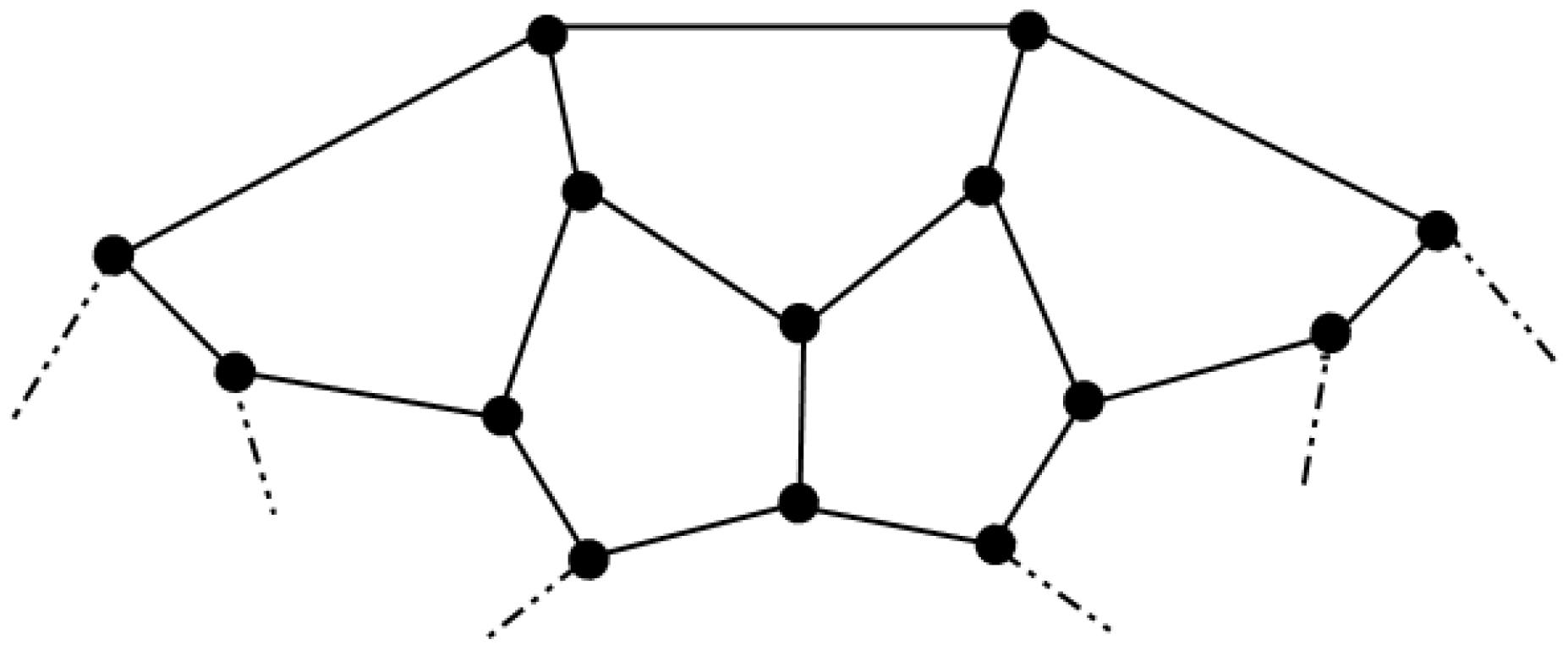
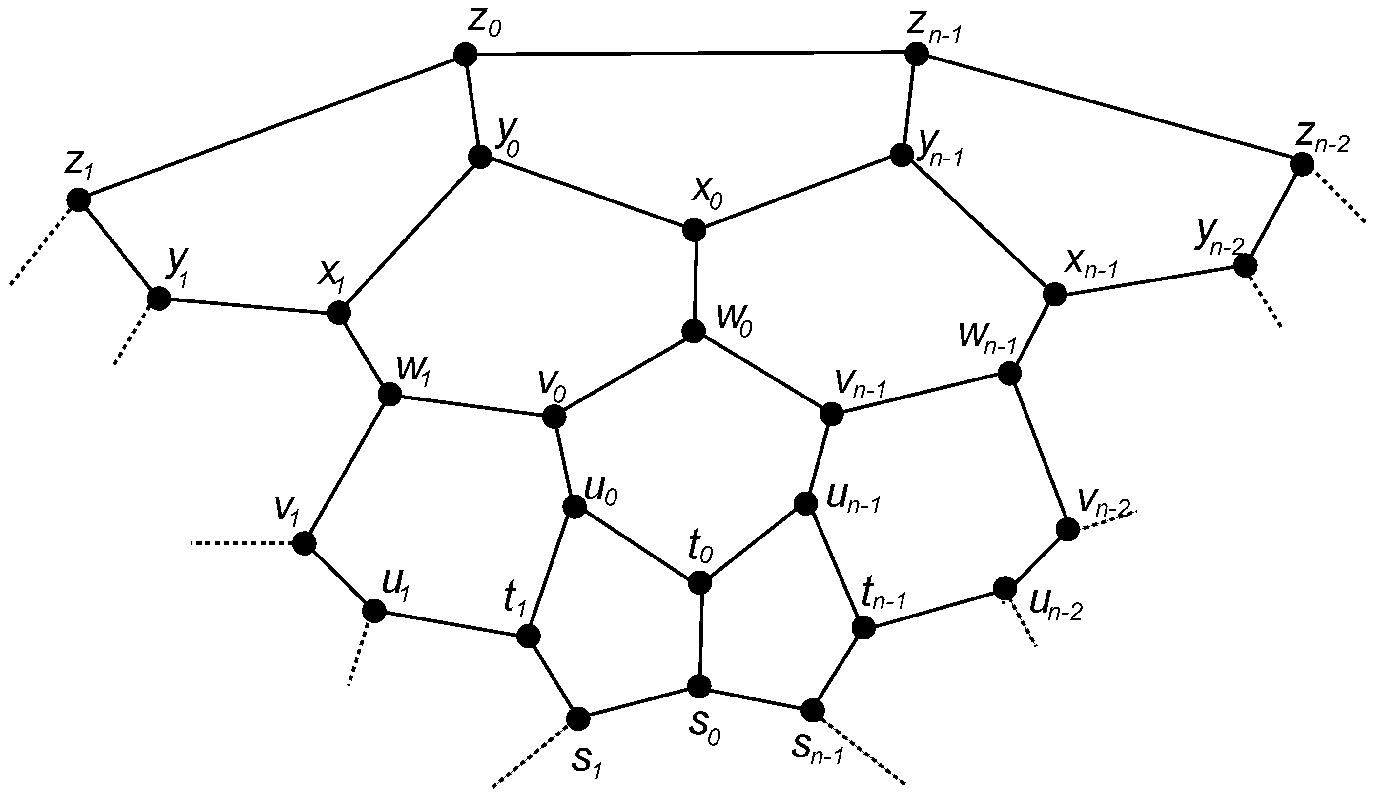
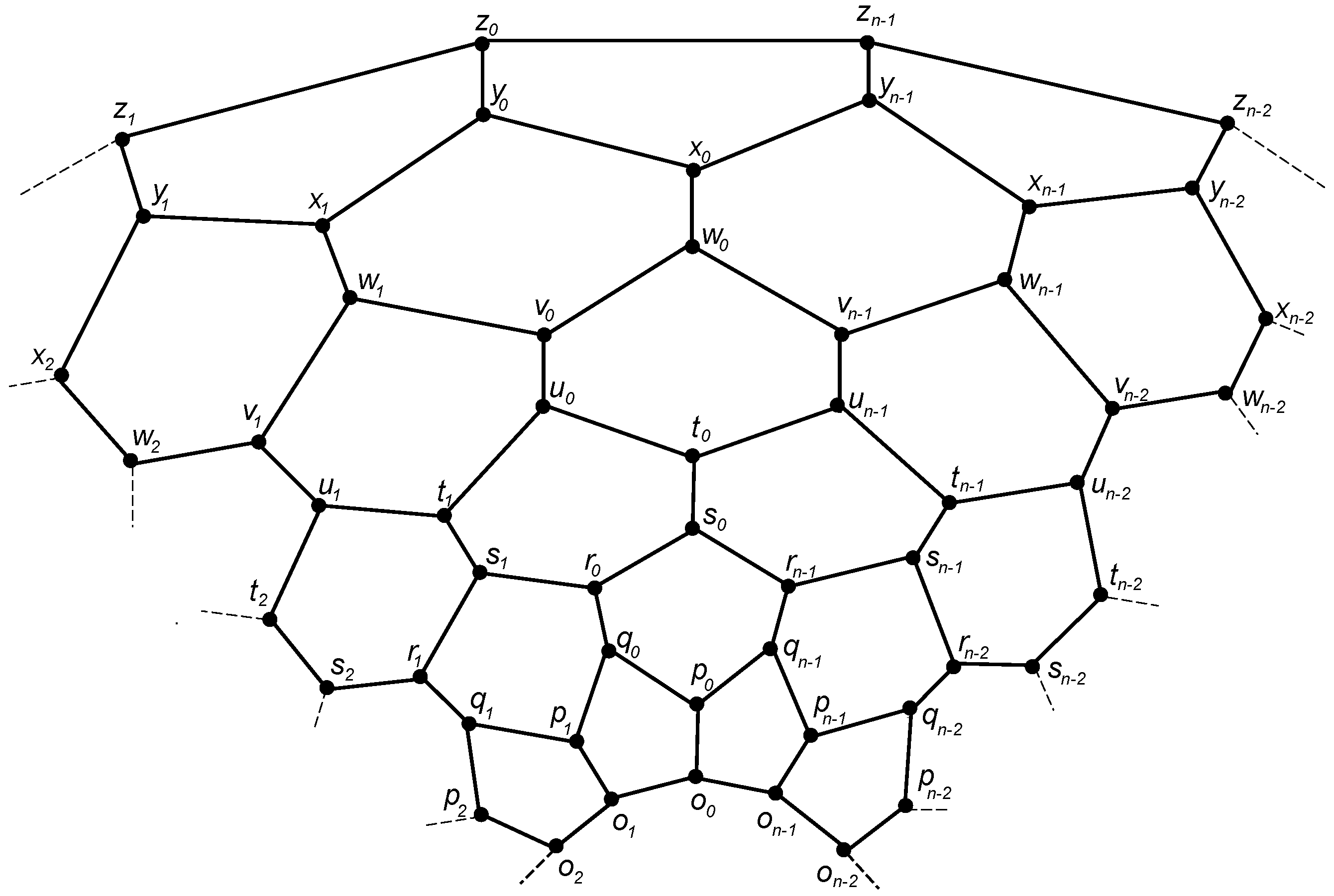
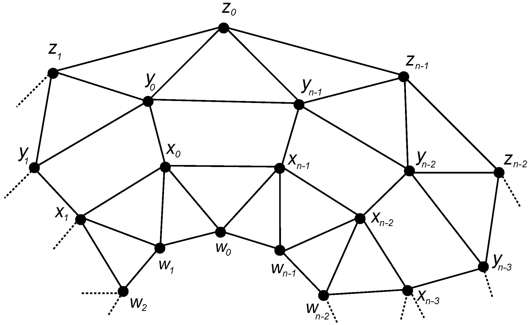
3.1. The Graph of Convex Polytope $H_n$

3.1.1. Construction

In 1999, Bača [31] studied the labeling problem of a family of convex polytopes denoted by ${\mathbb{B}}_n$ ($n\ge 3$). Figure 1 depicts the graph of convex polytope ${\mathbb{B}}_n$. Imran and Siddiqui [32] studied a variation of ${\mathbb{B}}_n$ by generalizing it to the family of two parametric convex polytope denoted by ${\mathbb{Q}}_n^m$, see [32], Figure 1. Note that the ${\mathbb{B}}_n$ is a special case of ${\mathbb{Q}}_n^m$ with $m=2$.

For a given planar graph G, the dual of G denoted by $du(G)$ is obtained by adding a vertex in each internal face of G and then joining any two of them if their corresponding faces share an edge. Miller et al. [33] considered another variation of ${\mathbb{B}}_n$ by defining its dual. They denoted this new family of polytopes with $R_n$. Figure 2 shows the graph of $R_n$.

Note that the family $R_n$ can also be obtained by adding a layer of hexagons between two pentagonal layers in the graph of $D_n$. The graph of $D_n$ can be viewed in Figure 3. Miller et al. [33] studied the vertex-magic total labeling of $R_n$. Imran et al. [34] studied the minimum metric dimension problem for the family of $R_n$.

In this paper, we propose two further variations of $D_n$ and study their binary locating-dominating number. In a similar fashion to Miller et al. [33], we add an extra layer of hexagons between the lower hexagonal layer and the outer pentagonal layer. We denote this new family of convex polytope with $H_n$. Figure 4 depicts the graph of convex polytope $H_n$. The weights’ assignment to the vertices in Figure 4 helps to trace the binary locating-dominating sets in this family of convex polytopes.

The graph of convex polytope $H_n$ comprises $2n$ pentagonal faces, $2n$ hexagonal faces and a pair of n-gonal faces.

Mathematically, the graph of convex polytope $H_n$ consists of the vertex set

$$V(H_n)=\{s_j,t_j,u_j,v_j,w_j,x_j,y_j,z_j\mid j=0,\dots ,n-1\}$$

(7)

and the edge set

$$E(H_n)=\{s_j{s}_{j+1},s_j{t}_j,t_j{u}_j,u_j{t}_{j+1},u_j{v}_j,v_j{w}_j,v_j{w}_{j+1},w_j{x}_j,x_j{y}_j,x_{j+1}{y}_j,y_j{z}_j,z_j{z}_{j+1}\mid j=0,\dots ,n-1\}.$$

(8)

Note that arithmetic in the subscripts is performed modulo n.

Next, we validate the vertex and edge sets of the convex polytope $H_n$. In order to do that, we fix $n=6$ and draw the graph $H_6$. According to expressions (7) and (8), we obtain the following vertex and edge sets for $H_6$:

$$V(H_6)=\{s_0,\dots ,s_5,t_0,\dots ,t_5,u_0,\dots ,u_5,v_0,\dots ,v_5,w_0,\dots ,w_5,x_0,\dots ,x_5,y_0,\dots ,y_5,z_0,\dots ,z_5\},$$

$$\begin{array}{ccc}\hfill E(H_6)& =& \{s_0{s}_1,s_1{s}_2,s_2{s}_3,s_3{s}_4,s_4{s}_5,s_5{s}_0,s_0{t}_0,s_1{t}_1,s_2{t}_2,s_3{t}_3,s_4{t}_4,s_5{t}_5,t_0{u}_0,t_1{u}_1,t_2{u}_2,t_3{u}_3,t_4{u}_4,t_5{u}_5,\hfill \\ & & u_0{t}_1,u_1{t}_2,u_2{t}_3,u_3{t}_4,u_4{t}_5,u_5{t}_0,u_0{v}_0,u_1{v}_1,u_2{v}_2,u_3{v}_3,u_4{v}_4,u_5{v}_5,v_0{w}_0,v_1{w}_1,v_2{w}_2,v_3{w}_3,\hfill \\ & & v_4{w}_4,v_5{w}_5,v_0{w}_1,v_1{w}_2,v_2{w}_3,v_3{w}_4,v_4{w}_5,v_5{w}_0,w_0{x}_0,w_1{x}_1,w_2{x}_2,w_3{x}_3,w_4{x}_4,w_5{x}_5,x_0{y}_0,\hfill \\ & & x_1{y}_1,x_2{y}_2,x_3{y}_3,x_4{y}_4,x_5{y}_5,y_0{x}_1,y_1{x}_2,y_2{x}_3,y_3{x}_4,y_4{x}_5,y_5{x}_0,y_0{z}_0,y_1{z}_1,y_2{z}_2,y_3{z}_3,\hfill \\ & & y_4{z}_4,y_5{z}_5,z_0{z}_1,z_1{z}_2,z_2{z}_3,z_3{z}_4,z_4{z}_5,z_5{z}_0\}.\hfill \end{array}$$

By using these vertex and edge sets, we construct the graph of the convex polytope $H_6$. Figure 5 shows the graph of $H_6$. This validates the vertex and edge sets presented in Equations (7) and (8).

The following problems are open for this newly proposed family of convex polytopes.

Problem 1.

Let G be the family of convex polytopes $H_n$, where $n\ge 3$ is an integer. Then,

(1) 

Study vertex-face magic, edge-face magic, vertex-face anti-magic, edge-face anti-magic and vertex/edge total labeling of G. See the references [15,16,31,33] for similar research on other family of convex polytopes.

(2) 

Study the minimum metric dimension problem for G. This problem is studied in [17,18,19,32,34] for other families of regular and non-regular convex polytopes.

(3) 

Study fault-tolerant resolvability of G. A similar study for other classes of convex polytopes is conducted by Raza et al. [35] and Salman et al. [22].

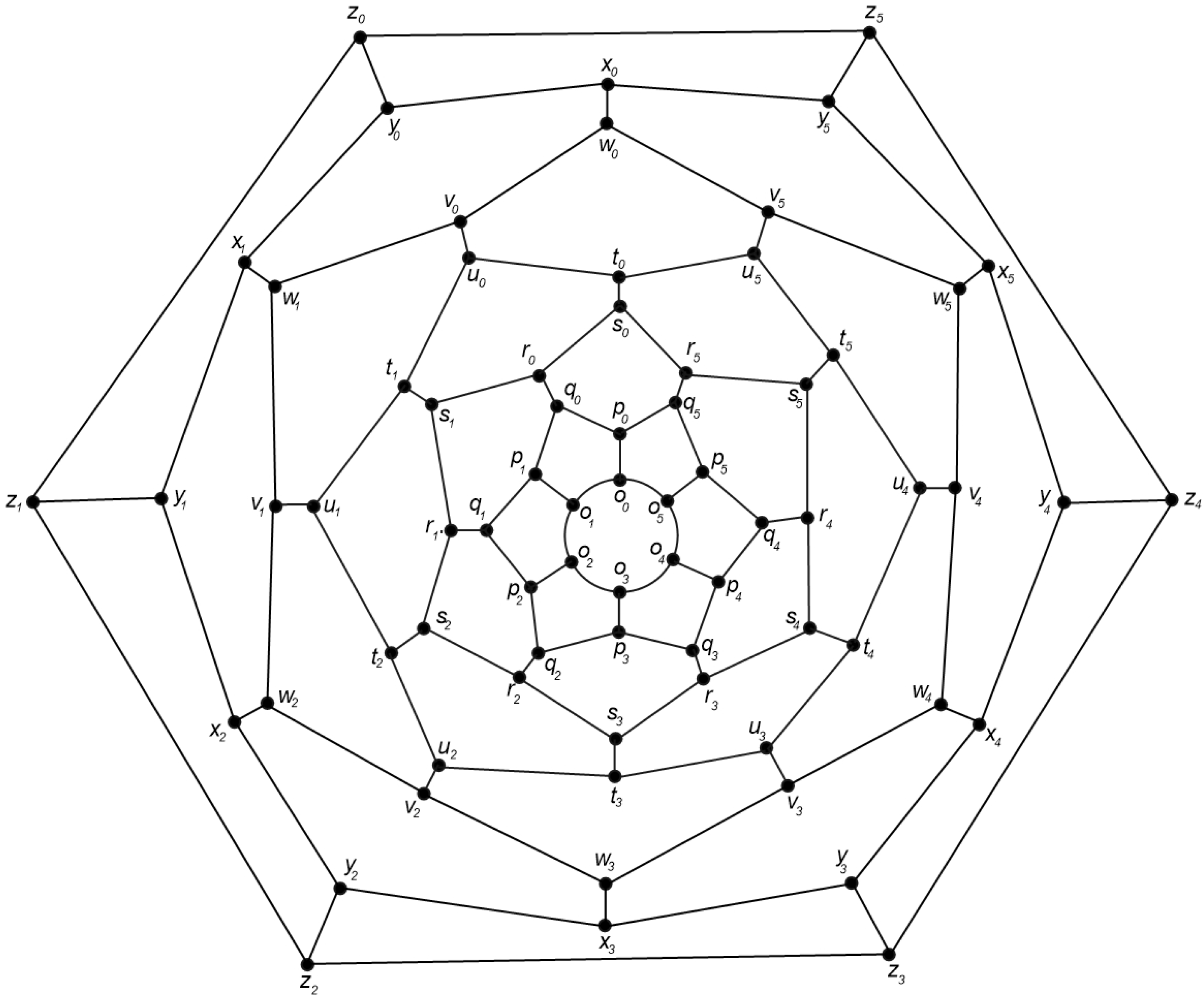
3.1.2. Rotational Symmetry of the Convex Polytopes

The convex polytopes considered in this paper possess two kind of rotational symmetries: one is geometrical symmetry and the other is structural symmetry. By geometrical symmetry, we mean the symmetry possessed by the underlying geometrical convex polytopes. By structural symmetry, we mean the symmetry of the graphs of the underlying convex polytopes. We discuss both of these symmetries in details.

Erickson and Kim [36] studied various geometrical properties of certain convex polytopes. One of the perspectives of his study is different symmetries possessed by certain classes of convex polytopes. In particular, they showed the following result:

Theorem 2.

For any integer positive integer n, there is a neighborly family of n congruent convex 3-polytopes, each with a plane of bilateral symmetry, a line of 180$°$ rotational symmetry, and a point of central symmetry.

Let ${\mathcal{H}}_n$ denote the infinite point set {$h_n(t)\mid t\in \mathbb{Z}\}$. The rotational symmetry is based on the fact that: a 180$°$ rotation about the y-axis maps $h_n(t)$ to $h_n(-t)$ and thus preserves the point set ${\mathcal{H}}_n$. This implies that the Voronoi region of the underlying polytope is rotationally symmetric about the y-axis. Erickson and Kim [36] used the symmetry group of the convex polytope to show Theorem 2. In this scenario, the underlying geometrical shapes of convex polytopes considered in this paper possess rotational symmetry studied by Erickson and Kim [36].

Now, we discuss the structural symmetry possessed by the graphs of the convex polytopes considered in this paper. By structure-wise rotational symmetry, we mean that a fixed unit of a convex polytope can be rotated along a circle, by following the structural similarity, to obtain the complete graph of the convex polytope. Let us fixed a convex polytope, say $H_n$ studied in the next subsubsection. In Figure 6, a unit of the graph of convex polytope $H_n$ is presented. By rotating this unit along the dotted circle with center O, we can obtain the whole graph $H_n$. The part with bold edges shows the unit of this convex polytope, which is rotated along the dotted circle. The complete graph is obtained by completing one revolution of the unit (bold part) along the dotted circle having center O.

Note that this graph-theoretic structural similarity is common among all the families of convex polytopes considered in the subsequent subsections.

3.1.3. Binary Locating-Dominating Number of $H_n$

In this subsubsection, we present the main result for the family of convex polytope $H_n$. We find the exact value of the binary locating-dominating number for this family of convex polytope.

The following theorem presents the exact value of the binary locating-dominating number of $H_n$.

Theorem 3.

The binary locating-dominating number of $H_n$ is given by the following expression:

$${\gamma }_{l-d}(H_n)=⌈\frac{8n}{3}⌉.$$

Proof. 

Note that $H_n$ is a family of regular graphs of degree 3 on $8n$ vertices. By Theorem 1, we find the following lower bound on the binary locating-dominating number of $H_n$:

$${\gamma }_{l-d}(H_n)\ge ⌈\frac{2(8n)}{6}⌉=⌈\frac{8n}{3}⌉.$$

(9)

Let S be a subset of the vertex set of $H_n$, such that

$$S=\left\{\begin{array}{cc}\{s_{3j+1},t_{3j},u_{3j+1},v_{3j+2},w_{3j+1},x_{3j+2},y_{3j},z_{3j+2}\mid j=0,\dots ,m-1\},\hfill & n=3m;\hfill \\ \{s_{3j+2},t_{3j},u_{3j+1},v_{3j},w_{3j+2},x_{3j+1},y_{3j+2},z_{3j}\}\bigcup \hfill & \\ \{t_{3m},v_{3m},y_{3m}\mid j=0,\dots ,m-1\},\hfill & n=3m+1;\hfill \\ \{s_{3j},t_{3j+1},u_{3j+2},v_{3j},w_{3j+2},x_{3j+1},y_{3j+2},z_{3j+1}\}\bigcup \hfill & \\ \{s_{3m},t_{3m+1},v_{3m},w_{3m+1},y_{3m+1},z_{3m}\mid j=0,\dots ,m-1\},\hfill & n=3m+2.\hfill \end{array}\right.$$

Next, we show that S is a binary locating-dominating set of $H_n$. In order to prove that, we need to discuss the following three possible cases:

Case 1:

When $n=3m$.

In order to show S to be a binary locating-dominating set, we need to show that the neighborhoods of all vertices in $V\backslash S$ are non-empty and distinct.

Table 1. Binary locating-dominating vertices in $H_n$.

n	$\mathit{v}\in \mathit{V}\backslash$S	$\mathit{S}\cap \mathit{N}[\mathit{v}]$	$\mathit{v}\in \mathit{V}\backslash$S	$\mathit{S}\cap \mathit{N}[\mathit{v}]$
$3m$	$s_{3j}$	$\{s_{3j+1},t_{3j}\}$	$s_{3j+2}$	$\{s_{3j+1}\}$
	$t_{3j+1}$	$\{s_{3j+1},u_{3j+1}\}$	$t_{3j+2}$	$\{u_{3j+1}\}$
	$u_{3j}$	$\{t_{3j}\}$	$u_{3j+2}$	$\{t_{3(j+1)},v_{3j+2}\}$
	$v_{3j}$	$\{w_{3j+1}\}$	$v_{3j+1}$	$\{w_{3j+1},u_{3j+1}\}$
	$w_{3j}$	$\{v_{3j-1}\}$	$w_{3j+2}$	$\{v_{3j+2},x_{3j+2}\}$
	$x_{3j}$	$\{y_{3j}\}$	$x_{3j+1}$	$\{y_{3j},w_{3j+1}\}$
	$y_{3j+1}$	$\{x_{3j+2}\}$	$y_{3j+2}$	$\{x_{3j+2},z_{3j+2}\}$
	$z_{3j}$	$\{y_{3j},z_{3j-1}\}$	$z_{3j+1}$	$\{z_{3j+2}\}$
$3m+1$	$s_{3j+1}$	$\{s_{3j+2}\}$	$s_{3(j+1)}$	$\{s_{3j+2},t_{3(j+1)}\}$
	$t_{3j+1}$	$\{u_{3j+1}\}$	$t_{3j+2}$	$\{u_{3j+1},s_{3j+2}\}$
	$u_{3j}$	$\{t_{3j},v_{3j}\}$	$u_{3j+2}$	$\{t_{3(j+1)}\}$
	$v_{3j+1}$	$\{u_{3j+1},w_{3j+2}\}$	$v_{3j+2}$	$\{w_{3j+2}\}$
	$w_{3j+1}$	$\{v_{3j},x_{3j+1}\}$	$w_{3(j+1)}$	$\{v_{3(j+1)}\}$
	$x_{3j+2}$	$\{w_{3j+2},y_{3j+2}\}$	$x_{3(j+1)}$	$\{y_{3j+2}\}$
	$y_{3j}$	$\{x_{3j+1},z_{3j}\}$	$y_{3j+1}$	$\{x_{3j+1}\}$
	$z_{3j+2}$	$\{y_{3j+2},z_{3j+3}\}$	$z_{3j+1}$	$\{z_{3j}\}$
	$s_0$	$\{t_0\}$	$u_{3m}$	$\{t_0,t_{3m},v_{3m}\}$
	$w_0$	$\{v_0,v_{3m}\}$	$x_0$	$\{y_{3m}\}$
	$z_{3m}$	$\{y_{3m},z_0\}$
$3m+2$	$s_{3j+1}$	$\{s_{3j},t_{3j+1}\}$	$s_{3j+2}$	$\{s_{3(j+1)}\}$
	$t_{3j+2}$	$\{u_{3j+2}\}$	$t_{3(j+1)}$	$\{s_{3(j+1)},u_{3j+2}\}$
	$u_{3j}$	$\{t_{3j+1},v_{3j}\}$	$u_{3j+1}$	$\{t_{3j+1}\}$
	$v_{3j+1}$	$\{w_{3j+2}\}$	$v_{3j+2}$	$\{u_{3j+2},w_{3j+2}\}$
	$w_{3j}$	$\{v_{3j}\}$	$w_{3j+1}$	$\{v_{3j},x_{3j+1}\}$
	$x_{3j+2}$	$\{w_{3j+2},y_{3j+2}\}$	$x_{3(j+1)}$	$\{y_{3j+2}\}$
	$y_{3j+1}$	$\{x_{3j+1},z_{3j+1}\}$	$y_{3j}$	$\{x_{3j+1}\}$
	$z_{3j}$	$\{z_{3j+1}\}$	$z_{3j+2}$	$\{y_{3j+2},z_{3j+1}\}$
	$s_{3m+1}$	$\{s_{3m},s_0,t_{3m+1}\}$	$t_0$	$\{s_0\}$
	$u_{3m+1}$	$\{t_{3m+1}\}$	$u_{3m}$	$\{t_{3m+1},v_{3m}\}$
	$v_{3m+1}$	$\{w_{3m+1}\}$	$w_{3m}$	$\{v_{3m}\}$
	$x_0$	$\{y_{3m+1}\}$	$x_{3m+1}$	$\{w_{3m+1},y_{3m+1}\}$
	$y_{3m}$	$\{z_{3m}\}$	$z_{3m+1}$	$\{y_{3m+1},z_{3m}\}$

shows these neighborhoods and their intersections. Although some formulas for some intersections can be somewhat similar, but they are distinct.

Case 2:

When $n=3m+1$.

As in the previous case, the neighborhoods of all vertices in $V\backslash S$ are non-empty and distinct shown in Table 1.

Case 3:

When $n=3m+2$.

Similar to the previous two cases, Table 1 shows that the neighborhoods of all vertices in $V\backslash S$ are non-empty and distinct.

It is easily seen that $\left|S\right|=⌈\frac{8n}{3}⌉$. This shows that

$${\gamma }_{l-d}(H_n)\le ⌈\frac{8n}{3}⌉.$$

(10)

By combining Inequalities (9) and (10), we obtain the result. □

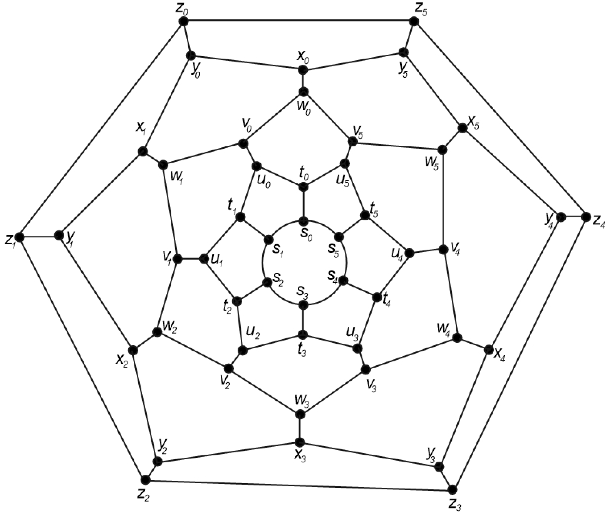
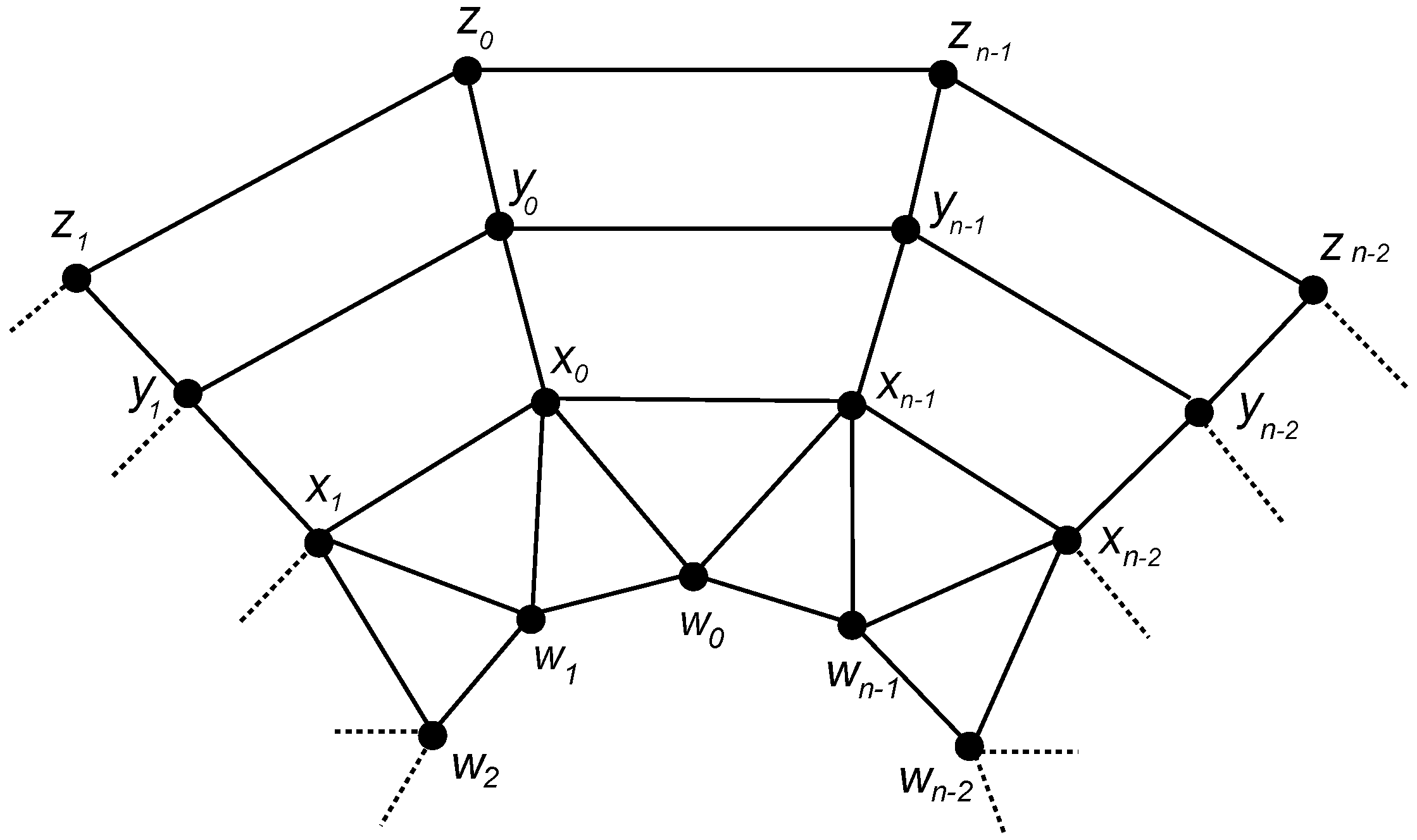
3.2. The Graph of Convex Polytope $H_n^{\prime }$

3.2.1. Construction

By following the same construction as for $H_n$, we define another variation of convex polytopes $R_n$ and $D_n$. We add an extra layer of hexagons between the outer pentagonal layer and the next hexagonal layer of $H_n$. In other words, $H_n^{\prime }$ can be obtained by adding three hexagonal layers in $R_n$ between outer pentagonal and inner hexagonal layers and four hexagonal layers in $D_n$ between the two pentagonal layers.

The graph of convex polytope $H_n$ comprises $2n$ pentagonal faces, $4n$ hexagonal faces and a pair of n-gonal faces. Figure 7 shows the graph of this family of convex polytopes. Mathematically, it has the vertex set

$$V(H_n^{\prime })=\{o_j,p_j,q_j,r_j,s_j,t_j,u_j,v_j,w_j,x_j,y_j,z_j\mid j=0,\dots ,n-1\},$$

(11)

and the edge set

$$\begin{array}{ccc}\hfill E(H_n^{\prime })& =& \{o_j{o}_{j+1},o_j{p}_j,q_j{p}_j,q_j{p}_{j+1},q_j{r}_j,r_j{s}_j,r_j{s}_{j+1},s_j{t}_j,t_j{u}_j,t_{j+1}{u}_j,u_j{v}_j,\hfill \\ & & v_j{w}_j,v_j{w}_{j+1},w_j{x}_j,x_j{y}_j,x_{j+1}{y}_j,y_j{z}_j,z_j{z}_{j+1}\mid j=0,\dots ,n-1\}.\hfill \end{array}$$

(12)

Note that arithmetic in the subscripts is performed modulo n.

Next, we validate the vertex and edge cardinalities of the graph of convex polytope $H_n^{\prime }$. We do that by fixing a value of $n=6$, and we construct the graph of $H_6^{\prime }$ from (11) and (12). We obtain the following vertex and edge set cardinalities for $H_6^{\prime }$:

$$\begin{array}{ccc}\hfill V(H_6^{\prime })& =& \{o_0,\dots ,o_5{p}_0,\dots ,p_5{q}_0,\dots ,q_5{r}_0,\dots ,r_5{s}_0,\dots ,s_5,t_0,\dots ,t_5,u_0,\dots ,u_5,v_0,\dots ,v_5,w_0,\dots ,w_5,\hfill \\ & & x_0,\dots ,x_5,y_0,\dots ,y_5,z_0,\dots ,z_5\},\hfill \end{array}$$

$$\begin{array}{ccc}\hfill E(H_6^{\prime })& =& \{o_0{o}_1,o_1{o}_2,o_2{o}_3,o_3{o}_4,o_4{o}_5,o_5{o}_0,o_0{p}_0,o_1{p}_1,o_2{p}_2,o_3{p}_3,o_4{p}_4,o_5{p}_5,p_0{q}_0,p_1{q}_1,p_2{q}_2,p_3{q}_3,\hfill \\ & & p_4{q}_4,p_5{q}_5,q_0{p}_1,q_1{p}_2,q_2{p}_3,q_3{p}_4,q_4{p}_5,q_5{p}_0,q_0{r}_0,q_1{r}_1,q_2{r}_2,q_3{r}_3,q_4{r}_4,q_5{r}_5,s_0{r}_0,s_1{r}_1,s_2{r}_2,\hfill \\ & & s_3{r}_3,s_4{r}_4,s_5{r}_5,r_0{s}_1,r_1{s}_2,r_2{s}_3,r_3{s}_4,r_4{s}_5,r_4{s}_0,s_0{t}_0,s_1{t}_1,s_2{t}_2,s_3{t}_3,s_4{t}_4,s_5{t}_5,t_0{u}_0,t_1{u}_1,t_2{u}_2,\hfill \\ & & t_3{u}_3,t_4{u}_4,t_5{u}_5,u_0{t}_1,u_1{t}_2,u_2{t}_3,u_3{t}_4,u_4{t}_5,u_5{t}_0,u_0{v}_0,u_1{v}_1,u_2{v}_2,u_3{v}_3,u_4{v}_4,u_5{v}_5,v_0{w}_0,\hfill \\ & & v_1{w}_1,v_2{w}_2,v_3{w}_3,v_4{w}_4,v_5{w}_5,v_0{w}_1,v_1{w}_2,v_2{w}_3,v_3{w}_4,v_4{w}_5,v_5{w}_0,w_0{x}_0,w_1{x}_1,w_2{x}_2,w_3{x}_3,\hfill \\ & & w_4{x}_4,w_5{x}_5,x_0{y}_0,x_1{y}_1,x_2{y}_2,x_3{y}_3,x_4{y}_4,x_5{y}_5,y_0{x}_1,y_1{x}_2,y_2{x}_3,y_3{x}_4,y_4{x}_5,y_5{x}_0,y_0{z}_0,\hfill \\ & & y_1{z}_1,y_2{z}_2,y_3{z}_3,y_4{z}_4,y_5{z}_5,z_0{z}_1,z_1{z}_2,z_2{z}_3,z_3{z}_4,z_4{z}_5,z_5{z}_0\}.\hfill \end{array}$$

By using these vertex and edge sets, we construct the graph of the convex polytope $H_6^{\prime }$. Figure 8 shows the graph of $H_6^{\prime }$. This validates the vertex and edge sets presented in (11) and (12).

3.2.2. Binary Locating-Dominating Number of $H_n^{\prime }$

This subsubsection presents the main result for $H_n^{\prime }$. We find the exact value of the the binary locating-dominating number of $H_n^{\prime }$. In the following theorem, it is shown that the binary locating-dominating number of the family $H_n^{\prime }$ is exactly $4n$.

Theorem 4.

The binary locating-dominating number of $H_n^{\prime }$ is exactly $4n$, i.e.,

$$\begin{array}{c}\hfill {\gamma }_{l-d}(H_n^{\prime })=4n.\end{array}$$

Proof. 

As the graph $H_n^{\prime }$ is regular with degree 3. By Theorem 1, we obtain

$$\begin{array}{c}\hfill {\gamma }_{l-d}\ge ⌈\frac{2(12n)}{6}⌉=4n.\end{array}$$

Let $S\subset V(H_n^{\prime })$ such that $S=\{p_j,s_j,v_j,y_j\mid j=0,\dots ,n-1\}$. Next, we show that S is a binary locating-dominating number of $H_n^{\prime }$. It can be seen that

$$\begin{array}{c}S\cap N[o_j]=[p_j],S\cap N[q_j]=[p_{j-1},p_j],S\cap N[r_j]=[s_j,s_{j+1}],S\cap N[t_j]=[s_j],S\cap N[u_j]=[v_j],\hfill \\ \hfill S\cap N[w_j]=[v_{j-1},v_j],S\cap N[x_j]=[y_{j-1},y_j]\mathrm{and}S\cap N[z_j]=[y_j].\end{array}$$

Note that all these intersections have at least one element and they are distinct as well. This shows that S is a binary locating dominating set of $(H_n^{\prime })$ and therefore ${\gamma }_{l-d}(H_n^{\prime })\le 4n$. By combining it with the fact ${\gamma }_{l-d}(H_n^{\prime })\ge 4n$, we obtain that ${\gamma }_{l-d}(H_n^{\prime })=4n$. □

4. Tight Upper Bounds

In this section, we find tight upper bounds on the binary locating-dominating number of three infinite families of convex polytopes.

4.1. The Graph of Convex Polytope $S_n$

The graph of convex polytope $S_n$ consists of $2n$ trigonal faces, $2n$ 4-gonal faces and a pair of n-sided faces (see Figure 9). Mathematically, it has the vertex set

$$V(S_n)=\{w_j,x_j,y_j,z_j\mid j=0,\dots ,n-1\},$$

and the edge set

$$E(S_n)=\{w_j{w}_{j+1},x_j{x}_{j+1},y_j{y}_{j+1},z_j{z}_{j+1}\mid j=0,\dots ,n-1\}\cup \{w_{j+1}{x}_j,w_j{x}_j,x_j{y}_j,y_j{z}_j\mid j=0,\dots ,n-1\}.$$

Imran et al. [19] showed that the metric dimension of $S_n$ is 3. The graph of convex polytope $S_n$ can also be obtained from the graph of convex polytope $Q_n$, defined in [16], by adding the edges $w_{j+1}{x}_j,y_j{y}_{j+1}$ and then deleting the edges $x_{j+1},y_j$ i.e., $V(S_n)=V(Q_n)$ and $E(S_n)=\left(E(Q_n)\cup \{w_{j+1}{x}_j,y_j{y}_{j+1}\mid j=0,\dots ,n-1\}\right)\backslash \{x_{j+1}{y}_j\mid j=0,\dots ,n-1\}$.

The following theorem gives a tight upper bound on the binary locating-dominating number of $S_n$.

Theorem 5.

Let G be the graph of convex polytope $S_n$. Then,

$${\gamma }_{l-d}(G)\le ⌈\frac{7n}{5}⌉,$$

and this upper bound is tight.

Proof. 

Let $S\subset V$ be a proper subset of the vertex set of $S_n$ such that

$$S=\left\{\begin{array}{cc}\{x_{5j},x_{5j+1},x_{5j+2},x_{5j+3},x_{5j+4},z_{5j+1},z_{5j+3}\mid j=0,\dots ,m-1\},\hfill & n=5m;\hfill \\ \{x_{5j},x_{5j+1},x_{5j+2},x_{5j+3},x_{5j+4},z_{5j+1},z_{5j+3}\bigcup \hfill & \\ \{x_{5m},z_{5m}\}\mid j=0,\dots ,m-1\},\hfill & n=5m+1;\hfill \\ \{x_{5j},x_{5j+1},x_{5j+2},x_{5j+3},x_{5j+4},z_{5j+1},z_{5j+3}\bigcup \hfill & \\ \{x_{5m},x_{5m+1},z_{5m+1}\}\mid j=0,\dots ,m-1\},\hfill & n=5m+2;\hfill \\ \{x_{5j},x_{5j+1},x_{5j+2},x_{5j+3},x_{5j+4},z_{5j+1},z_{5j+3}\bigcup \hfill & \\ \{x_{5m},x_{5m+1},x_{5m+2},z_{5m},z_{5m+2}\},\hfill & n=5m+3;\hfill \\ \{x_{5m},x_{5m+1},x_{5m+2},x_{5m+3},z_{5m+1},z_{5m+3}\}\bigcup \hfill & \\ \{x_{5j},x_{5j+1},x_{5j+2},x_{5j+3},x_{5j+4},z_{5j+1},z_{5j+3}\mid j=0,\dots ,m-1\},\hfill & n=5m+4.\hfill \end{array}\right.$$

Next, we show that S is a locating-dominating set of G. To do that, we discuss the following five possible cases:

Case 1:

When $n=5m$.

Table 2. Binary locating-dominating vertices in $S_n$.

n	$\mathit{v}\in \mathit{V}\backslash$S	$\mathit{S}\cap \mathit{N}[\mathit{v}]$	$\mathit{v}\in \mathit{V}\backslash$S	$\mathit{S}\cap \mathit{N}[\mathit{v}]$
$5m$	$w_{5j}$	$\{x_{5j},x_{5(j-1)+4}\}$	$w_{5j+1}$	$\{x_{5j},x_{5j+1}\}$
	$w_{5j+2}$	$\{x_{5j+1},x_{5j+2}\}$	$w_{5j+3}$	$\{x_{5j+2},x_{5j+3}\}$
	$w_{5j+4}$	$\{x_{5j+3},x_{5j+4}\}$	$y_{5j}$	$\{x_{5j}\}$
	$y_{5j+1}$	$\{x_{5j+1},z_{5j+1}\}$	$y_{5j+2}$	$\{x_{5j+2}\}$
	$y_{5j+3}$	$\{x_{5j+3},z_{5j+3}\}$	$y_{5j+4}$	$\{x_{5j+4}\}$
	$z_{5j}$	$\{z_{5j+1}\}$	$z_{5j+2}$	$\{z_{5j+1},z_{5j+3}\}$
	$z_{5j+4}$	$\{z_{5j+3}\}$
$5m+1$	$w_{5j+1}$	$\{x_{5j},x_{5j+1}\}$	$w_{5j+2}$	$\{x_{5j+1},x_{5j+2}\}$
	$w_{5j+3}$	$\{x_{5j+2},x_{5j+3}\}$	$w_{5j+4}$	$\{x_{5j+3},x_{5j+4}\}$
	$w_{5(j+1)}$	$\{x_{5j+4},x_{5(j+1)}\}$	$y_{5j}$	$\{x_{5j}\}$
	$y_{5j+1}$	$\{x_{5j+1},z_{5j+1}\}$	$y_{5j+2}$	$\{x_{5j+2}\}$
	$y_{5j+3}$	$\{x_{5j+3},z_{5j+3}\}$	$y_{5j+4}$	$\{x_{5j+4}\}$
	$z_{5j}$	$\{z_{5j+1}\}$	$z_{5j+2}$	$\{z_{5j+1},z_{5j+3}\}$
	$z_{5j+4}$	$\{z_{5j+3}\}$	$w_0$	$\{x_0,x_{5m}\}$
	$y_{5m}$	$\{x_{5m},z_{5m}\}$
$5m+2$	$w_{5j+1}$	$\{x_{5j},x_{5j+1}\}$	$w_{5j+2}$	$\{x_{5j+1},x_{5j+2}\}$
	$w_{5j+3}$	$\{x_{5j+2},x_{5j+3}\}$	$w_{5j+4}$	$\{x_{5j+3},x_{5j+4}\}$
	$w_{5(j+1)}$	$\{x_{5j+4},x_{5(j+1)}\}$	$y_{5j}$	$\{x_{5j}\}$
	$y_{5j+1}$	$\{x_{5j+1},z_{5j+1}\}$	$y_{5j+2}$	$\{x_{5j+2}\}$
	$y_{5j+3}$	$\{x_{5j+3},z_{5j+3}\}$	$y_{5j+4}$	$\{x_{5j+4}\}$
	$z_{5j}$	$\{z_{5j+1}\}$	$z_{5j+2}$	$\{z_{5j+1},z_{5j+3}\}$
	$z_{5j+4}$	$\{z_{5j+3}\}$	$w_0$	$\{x_0,x_{5m+1}\}$
	$w_{5m+1}$	$\{x_{5m},x_{5m+1}\}$	$y_{5m}$	$\{x_{5m}\}$
	$y_{5m+1}$	$\{x_{5m+1},z_{5m+1}\}$	$z_{5m}$	$\{z_{5m+1}\}$
$5m+3$	$w_{5j+1}$	$\{x_{5j},x_{5j+1}\}$	$w_{5j+2}$	$\{x_{5j+1},x_{5j+2}\}$
	$w_{5j+3}$	$\{x_{5j+2},x_{5j+3}\}$	$w_{5j+4}$	$\{x_{5j+3},x_{5j+4}\}$
	$w_{5(j+1)}$	$\{x_{5j+4},x_{5(j+1)}\}$	$y_{5j}$	$\{x_{5j}\}$
	$y_{5j+1}$	$\{x_{5j+1},z_{5j+1}\}$	$y_{5j+2}$	$\{x_{5j+2}\}$
	$y_{5j+3}$	$\{x_{5j+3},z_{5j+3}\}$	$y_{5j+4}$	$\{x_{5j+4}\}$
	$z_{5j}$	$\{z_{5j+1}\}$	$z_{5j+2}$	$\{z_{5j+1},z_{5j+3}\}$
	$z_{5j+4}$	$\{z_{5j+3}\}$	$w_0$	$\{x_0,x_{5m+2}\}$
	$w_{5m+1}$	$\{x_{5m},x_{5m+1}\}$	$w_{5m+2}$	$\{x_{5m+1},x_{5m+2}\}$
	$y_{5m}$	$\{x_{5m},z_{5m}\}$	$y_{5m+1}$	$\{x_{5m+1}\}$
	$y_{5m+2}$	$\{x_{5m+2},z_{5m+2}\}$	$z_{5m+1}$	$\{z_{5m},z_{5m+2}\}$
$5m+4$	$w_{5j+1}$	$\{x_{5j},x_{5j+1}\}$	$w_{5j+2}$	$\{x_{5j+1},x_{5j+2}\}$
	$w_{5j+3}$	$\{x_{5j+2},x_{5j+3}\}$	$w_{5j+4}$	$\{x_{5j+3},x_{5j+4}\}$
	$w_{5(j+1)}$	$\{x_{5j+4},x_{5(j+1)}\}$	$y_{5j}$	$\{x_{5j}\}$
	$y_{5j+1}$	$\{x_{5j+1},z_{5j+1}\}$	$y_{5j+2}$	$\{x_{5j+2}\}$
	$y_{5j+3}$	$\{x_{5j+3},z_{5j+3}\}$	$y_{5j+4}$	$\{x_{5j+4}\}$
	$z_{5j}$	$\{z_{5j+1}\}$	$z_{5j+2}$	$\{z_{5j+1},z_{5j+3}\}$
	$z_{5j+4}$	$\{z_{5j+3}\}$	$w_0$	$\{x_0,x_{5m+3}\}$
	$w_{5m+1}$	$\{x_{5m},x_{5m+1}\}$	$w_{5m+2}$	$\{x_{5m+1},x_{5m+2}\}$
	$w_{5m+3}$	$\{x_{5m+2},x_{5m+3}\}$	$y_{5m}$	$\{x_{5m}\}$
	$y_{5m+1}$	$\{x_{5m+1},z_{5m+1}\}$	$y_{5m+2}$	$\{x_{5m+2}\}$
	$y_{5m+3}$	$\{x_{5m+3},z_{5m+3}\}$	$z_{5m}$	$\{z_{5m+1}\}$
	$z_{5m+2}$	$\{z_{5m+1},z_{5m+3}\}$

depicts all vertices in $V\backslash$S and the intersections of their closed neighborhoods with S. From the second column, we can see that all these intersections are nonempty and distinct. Thus, for any two vertices $u,v\in V\backslash$S, we have $S\bigcap N[v]\ne S\bigcap N[u]\ne Ø$. This shows that S is a binary locating-dominating set of $S_n$.

Case 2:

When $n=5m+1$.

Similar to the argument in Case 1, we see from Table 2 that all the intersections are nonempty and distinct. This shows that S is a binary locating-dominating set for $S_n$, if $n=5m+1$.

Case 3:

When $n=5m+2$.

Similar to the argument in Case 1 and Case 2, we see from Table 2 that all the intersections are nonempty and distinct. This shows that S is a binary locating-dominating set for $S_n$, if $n=5m+2$.

Thus, from the above discussion, we can say that Case 4 and Case 5 are analogous to above mentioned cases.

Note that $\left|S\right|=⌈\frac{7n}{5}⌉$; therefore, we have ${\gamma }_{l-d}(G)\le ⌈\frac{7n}{5}⌉$.

In order to show tightness in the upper bound from Theorem 5, we use the CPLEX solver for the ILP formulation with constraints (1), (2), (4) and (6). As a result, we obtain the following optimal solutions: ${\gamma }_{l-d}(S_6)=9$, ${\gamma }_{l-d}(S_7)=10$, ${\gamma }_{l-d}(S_8)=12$, ${\gamma }_{l-d}(S_9)=13$, …, ${\gamma }_{l-d}(S_{21})=30$, …, ${\gamma }_{l-d}(S_{29})=41$. This shows the upper bound in Theorem 5 is tight. □

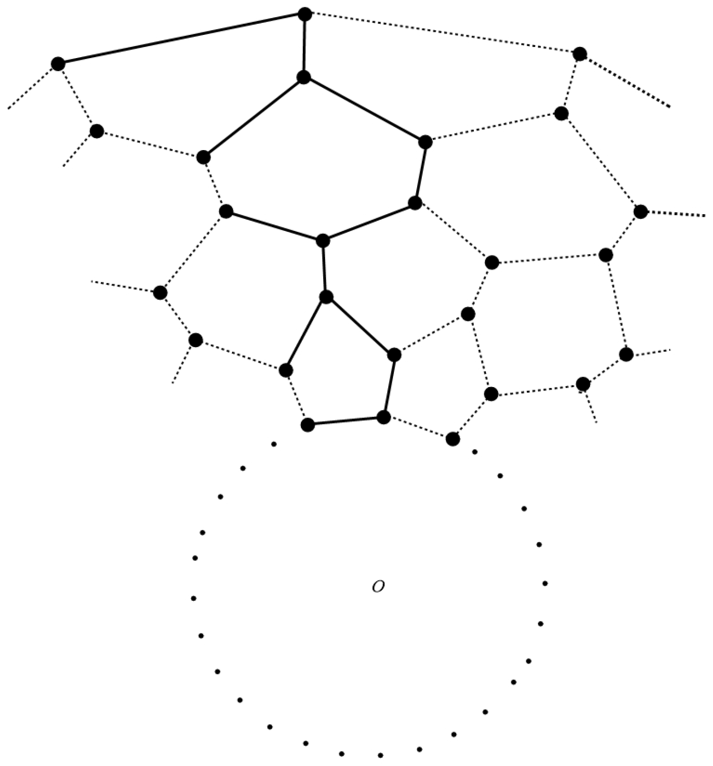
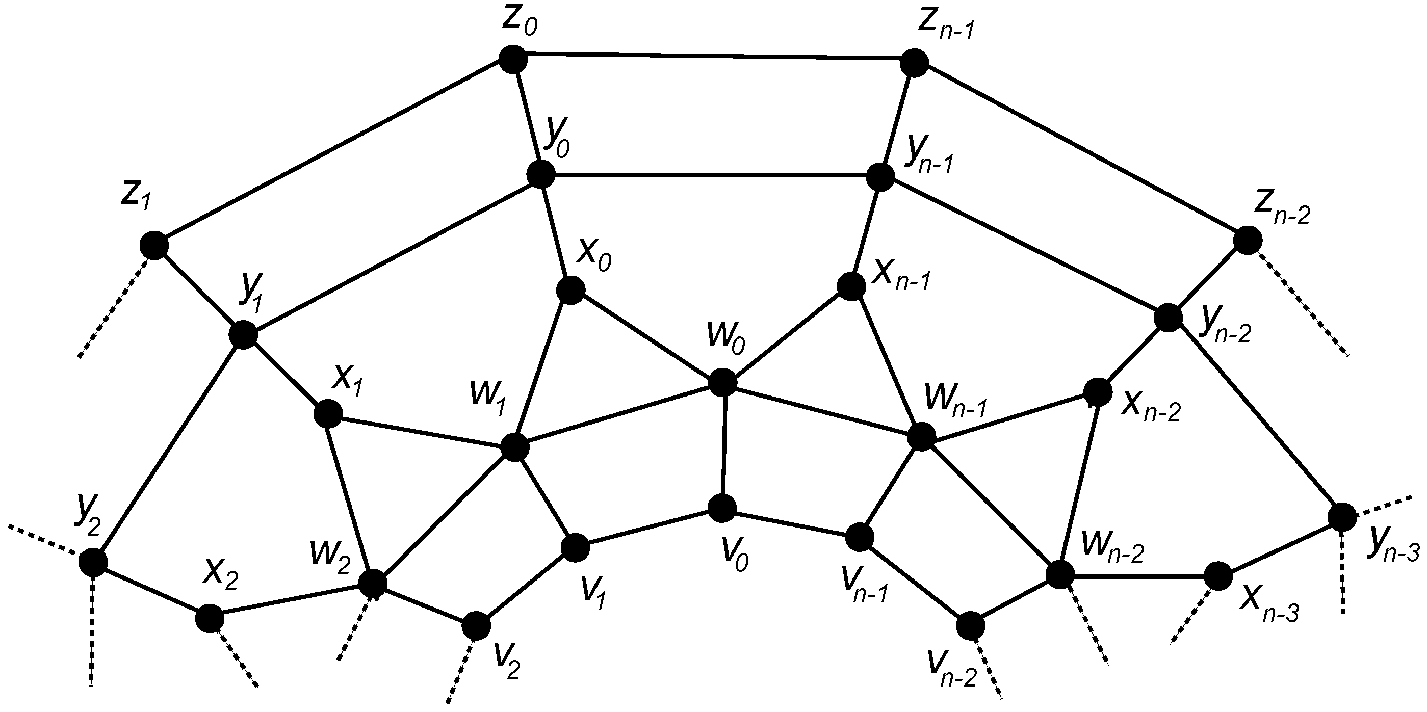
4.2. The Graph of Convex Polytope $B_n$

The graph of convex polytope $B_n$ comprises $2n$ 4-gonal faces, n trigonal faces, n pentagonal faces and a pair of n-gonal faces (see Figure 10). It can also be obtained by the combination of graph of convex polytope $Q_n$ [16] and a graph of prism $D_n$ [15]. Alternatively, it has the vertex set

$$V(B_n)=\{v_j,w_j,x_j,y_j,z_j\mid j=0,\dots ,n-1\},$$

and the edge set

$$\begin{array}{c}E(B_n)=\{v_j{v}_{j+1},w_j{w}_{j+1},y_j{y}_{j+1},z_j{z}_{j+1}\mid j=0,\dots ,n-1\}\cup \hfill \\ \{v_j{w}_j,w_j{x}_j,w_{j+1}{x}_j,x_j{y}_j,y_j{z}_j\mid j=0,\dots ,n-1\}.\hfill \end{array}$$

Imran et al. [18] showed that the metric dimension of the convex polytope $B_n$ is three. Next, we prove a tight upper bound on the binary locating-dominating number of $B_n$.

Theorem 6.

The binary locating-dominating number of $B_n$ is bounded above by $2n$, i.e.,

$${\gamma }_{l-d}(B_n)\le 2n,$$

and this upper bound is tight.

Proof. 

Let $S\subset V(B_n)$ such that $S=\{w_j,y_j\mid j=0,\dots ,n-1\}$. Next, we show that S is a binary locating-dominating number of $B_n$. It can be seen that

$$S\cap N[v_j]=[w_j],S\cap N[x_j]=[w_j,w_{j+1},y_j],\mathrm{and}S\cap N[z_j]=[y_j].$$

Note that all these intersections have at least one element and they are distinct as well. This shows that S is a binary locating-dominating set of $B_n$. Therefore, we obtain that ${\gamma }_{l-d}(G)\le 2n$.

Using the CPLEX solver on the integer linear programming formulation with constraints (1), (2), (4) and (6), we obtain the optimal solutions: ${\gamma }_{l-d}(B_7)=14$, ${\gamma }_{l-d}(B_8)=16$, ${\gamma }_{l-d}(B_9)=18$, …, ${\gamma }_{l-d}(S_{15})=30$. This shows that the upper bound is tight. □

4.3. The Graph of Convex Polytope $T_n$

The graph of convex polytope $T_n$ consists of $4n$ trigonal faces, n 4-gonal faces and a pair of n-sided faces (see Figure 11). Mathematically, we have

$$V(T_n)=\{w_j,x_j,y_j,z_j\mid j=0,\dots ,n-1\}$$

and

$$\begin{array}{c}E(T_n)=\{w_j{w}_{j+1},x_j{x}_{j+1},y_j{y}_{j+1},z_j{z}_{j+1}\mid j=0,\dots ,n-1\}\cup \hfill \\ \{w_{j+1}{x}_j,w_j{x}_j,x_j{y}_j,y_i{z}_j,y_{j+1}{z}_j\mid j=0,\dots ,n-1\}.\hfill \end{array}$$

It can also be obtained by the combination of the graph of convex polytope $R_n$ [15,19] and the graph of an antiprism.

Theorem 7.

For the graph of convex polytope $T_n$, we have

$${\gamma }_{l-d}(T_n)\le ⌈\frac{7n}{5}⌉,$$

and this upper bound is tight.

Proof. 

Let S be a proper subset of the vertex set of $T_n$, such that

$$S=\left\{\begin{array}{cc}\{x_{5j},x_{5j+1},x_{5j+2},x_{5j+3},x_{5j+4},z_{5j+1},z_{5j+3}\mid j=0,\dots ,m-1\},\hfill & n=5m;\hfill \\ \{x_{5j},x_{5j+1},x_{5j+2},x_{5j+3},x_{5j+4},z_{5j+1},z_{5j+3}\bigcup \hfill & \\ \{x_{5m},z_{5m}\}\mid j=0,\dots ,m-1\},\hfill & n=5m+1;\hfill \\ \{x_{5j},x_{5j+1},x_{5j+2},x_{5j+3},x_{5j+4},z_{5j+1},z_{5j+3}\bigcup \hfill & \\ \{x_{5m},x_{5m+1},z_{5m+1}\}\mid j=0,\dots ,m-1\},\hfill & n=5m+2;\hfill \\ \{x_{5j},x_{5j+1},x_{5j+2},x_{5j+3},x_{5j+4},z_{5j+1},z_{5j+3}\bigcup \hfill & \\ \{x_{5m},x_{5m+1},x_{5m+2},z_{5m},z_{5m+2}\},\hfill & n=5m+3;\hfill \\ \{x_{5m},x_{5m+1},x_{5m+2},x_{5m+3},z_{5m+1},z_{5m+3}\}\bigcup \hfill & \\ \{x_{5j},x_{5j+1},x_{5j+2},x_{5j+3},x_{5j+4},z_{5j+1},z_{5j+3}\mid j=0,\dots ,m-1\},\hfill & n=5m+4.\hfill \end{array}\right.$$

We show that S is a binary locating-dominating set of $T_n$. We need to discuss the following two possible cases:

Case 1:

When $n=5m$.

In order to show S to be a binary locating-dominating set, we need to show that the neighborhoods of all vertices in $V\backslash$S are non-empty and distinct.

Table 3. Binary locating-dominating vertices in $T_n$.

n	$\mathit{v}\in \mathit{V}\backslash$S	$\mathit{S}\cap \mathit{N}[\mathit{v}]$	$\mathit{v}\in \mathit{V}\backslash$S	$\mathit{S}\cap \mathit{N}[\mathit{v}]$
$5m$	$w_{5j}$	$\{x_{5j},x_{5(j-1)+4}\}$	$w_{5j+1}$	$\{x_{5j},x_{5j+1}\}$
	$w_{5j+2}$	$\{x_{5j+1},x_{5j+2}\}$	$w_{5j+3}$	$\{x_{5j+2},x_{5j+3}\}$
	$w_{5j+4}$	$\{x_{5j+3},x_{5j+4}\}$	$y_{5j}$	$\{x_{5j},z_{5j+1}\}$
	$y_{5j+1}$	$\{x_{5j+1},z_{5j+1}\}$	$y_{5j+2}$	$\{x_{5j+2},z_{5j+3}\}$
	$y_{5j+3}$	$\{x_{5j+3},z_{5j+3}\}$	$y_{5j+4}$	$\{x_{5j+4}\}$
	$z_{5j}$	$\{z_{5j+1}\}$	$z_{5j+2}$	$\{z_{5j+1},z_{5j+3}\}$
	$z_{5j+4}$	$\{z_{5j+3}\}$
$5m+1$	$w_{5j+1}$	$\{x_{5j},x_{5j+1}\}$	$w_{5j+2}$	$\{x_{5j+1},x_{5j+2}\}$
	$w_{5j+3}$	$\{x_{5j+2},x_{5j+3}\}$	$w_{5j+4}$	$\{x_{5j+3},x_{5j+4}\}$
	$w_{5(j+1)}$	$\{x_{5j+3},x_{5(j+1)}\}$	$y_{5j}$	$\{x_{5j},z_{5j+1}\}$
	$y_{5j+1}$	$\{x_{5j+1},z_{5j+1}\}$	$y_{5j+2}$	$\{x_{5j+2},z_{5j+3}\}$
	$y_{5j+3}$	$\{x_{5j+3},z_{5j+3}\}$	$y_{5j+4}$	$\{x_{5j+4}\}$
	$z_{5j}$	$\{z_{5j+1}\}$	$z_{5j+2}$	$\{z_{5j+1},z_{5j+3}\}$
	$z_{5j+4}$	$\{z_{5j+3}\}$	$w_0$	$\{x_0,x_{5m}\}$
	$y_{5m}$	$\{x_{5m},z_{5m}\}$
$5m+2$	$w_{5j+1}$	$\{x_{5j},x_{5j+1}\}$	$w_{5j+2}$	$\{x_{5j+1},x_{5j+2}\}$
	$w_{5j+3}$	$\{x_{5j+2},x_{5j+3}\}$	$w_{5j+4}$	$\{x_{5j+3},x_{5j+4}\}$
	$w_{5(j+1)}$	$\{x_{5j+3},x_{5(j+1)}\}$	$y_{5j}$	$\{x_{5j},z_{5j+1}\}$
	$y_{5j+1}$	$\{x_{5j+1},z_{5j+1}\}$	$y_{5j+2}$	$\{x_{5j+2},z_{5j+3}\}$
	$y_{5j+3}$	$\{x_{5j+3},z_{5j+3}\}$	$y_{5j+4}$	$\{x_{5j+4}\}$
	$z_{5j}$	$\{z_{5j+1}\}$	$z_{5j+2}$	$\{z_{5j+1},z_{5j+3}\}$
	$z_{5j+4}$	$\{z_{5j+3}\}$	$w_0$	$\{x_0,x_{5m+1}\}$
	$w_{5m+1}$	$\{x_{5m},x_{5m+1}\}$	$y_{5m}$	$\{x_{5m},z_{5m}\}$
	$y_{5m+1}$	$\{x_{5m+1},z_{5m}\}$	$z_{5m}$	$\{z_{5m+1}\}$
$5m+3$	$w_{5j+1}$	$\{x_{5j},x_{5j+1}\}$	$w_{5j+2}$	$\{x_{5j+1},x_{5j+2}\}$
	$w_{5j+3}$	$\{x_{5j+2},x_{5j+3}\}$	$w_{5j+4}$	$\{x_{5j+3},x_{5j+4}\}$
	$w_{5(j+1)}$	$\{x_{5j+3},x_{5(j+1)}\}$	$y_{5j}$	$\{x_{5j},z_{5j+1}\}$
	$y_{5j+1}$	$\{x_{5j+1},z_{5j+1}\}$	$y_{5j+2}$	$\{x_{5j+2},z_{5j+3}\}$
	$y_{5j+3}$	$\{x_{5j+3},z_{5j+3}\}$	$y_{5j+4}$	$\{x_{5j+4}\}$
	$z_{5j}$	$\{z_{5j+1}\}$	$z_{5j+2}$	$\{z_{5j+1},z_{5j+3}\}$
	$z_{5j+4}$	$\{z_{5j+3}\}$	$w_0$	$\{x_0,x_{5m+2}\}$
	$w_{5m+1}$	$\{x_{5m},x_{5m+1}\}$	$w_{5m+2}$	$\{x_{5m+1},x_{5m+2}\}$
	$y_{5m}$	$\{x_{5m},z_{5m}\}$	$y_{5m+1}$	$\{x_{5m+1},z_{5m+2}\}$
	$y_{5m+2}$	$\{x_{5m+2},z_{5m+2}\}$	$z_{5m+1}$	$\{z_{5m},z_{5m+2}\}$
$5m+4$	$w_{5j+1}$	$\{x_{5j},x_{5j+1}\}$	$w_{5j+2}$	$\{x_{5j+1},x_{5j+2}\}$
	$w_{5j+3}$	$\{x_{5j+2},x_{5j+3}\}$	$w_{5j+4}$	$\{x_{5j+3},x_{5j+4}\}$
	$w_{5(j+1)}$	$\{x_{5j+3},x_{5(j+1)}\}$	$y_{5j}$	$\{x_{5j},z_{5j+1}\}$
	$y_{5j+1}$	$\{x_{5j+1},z_{5j+1}\}$	$y_{5j+2}$	$\{x_{5j+2},z_{5j+3}\}$
	$y_{5j+3}$	$\{x_{5j+3},z_{5j+3}\}$	$y_{5j+4}$	$\{x_{5j+4}\}$
	$z_{5j}$	$\{z_{5j+1}\}$	$z_{5j+2}$	$\{z_{5j+1},z_{5j+3}\}$
	$z_{5j+4}$	$\{z_{5j+3}\}$	$w_0$	$\{x_0,x_{5m+2}\}$
	$w_{5m+1}$	$\{x_{5m},x_{5m+1}\}$	$w_{5m+2}$	$\{x_{5m+1},x_{5m+2}\}$
	$w_{5m+3}$	$\{x_{5m+2},x_{5m+3}\}$	$y_{5m}$	$\{x_{5m},z_{5m}\}$
	$y_{5m+1}$	$\{x_{5m+1},z_{5m+1}\}$	$y_{5m+2}$	$\{x_{5m+2},z_{5m+3}\}$
	$y_{5m+3}$	$\{x_{5m+3},z_{5m+3}\}$	$z_{5m}$	$\{z_{5m+1}\}$
	$z_{5m+2}$	$\{z_{5m+1},z_{5m+3}\}$

shows these neighborhoods and their intersections. Although some formulas for some intersections can be somewhat similar, but they are distinct.

Case 2:

When $n=5m+1$.

As in the previous case, the the neighborhoods of all vertices in $V\backslash$S are non-empty and distinct shown in Table 3. Thus, from the above discussion, we can say that Case 3, Case 4 and Case 5 are analogous to the above-mentioned cases.

Note that $\left|S\right|=⌈\frac{7n}{5}⌉$. This implies that ${\gamma }_{l-d}(T_n)\le ⌈\frac{7n}{5}⌉$.

Next, we use the CPLEX solver for the ILP formulation with constraints (1), (2), (4) and (6) and obtain the following optimal solutions: ${\gamma }_{l-d}(T_6)=9$, ${\gamma }_{l-d}(T_7)=10$, ${\gamma }_{l-d}(T_8)=12$, ${\gamma }_{l-d}(T_9)=13$, …, ${\gamma }_{l-d}(T_{21})=30$, …, ${\gamma }_{l-d}(T_{29})=41$. This shows the upper bound in Theorem 7 is tight. □

5. Conclusions

In this paper, we focus on a class of geometric graphs which naturally arise from the structures of convex polytopes. Besides finding exact values for the binary locating-dominating number of two infinite families of graphs of convex polytopes, we also find tight upper bounds on other three infinite families of convex polytopes. An integer linear programming model for binary locating-locating number is used to find tightness in the obtained upper bounds.

Generalized Petersen graphs and certain families of strongly regular graphs can be considered for further research on this problem.

References

1. Haynes, T.W.; Hedetniemi, S.; Slater, P. Fundamentals of Domination in Graphs; CRC Press: Boca Raton, FL, USA, 1998. [Google Scholar]
2. Haynes, T.W.; Henning, M.A.; Howard, J. Locating and total dominating sets in trees. Discret. Appl. Math. 2006, 154, 1293–1300. [Google Scholar] [CrossRef] [Green Version]
3. Charon, I.; Hudry, O.; Lobstein, A. Extremal cardinalities for identifying and locating-dominating codes in graphs. Discret. Math. 2007, 307, 356–366. [Google Scholar] [CrossRef]
4. Honkala, I.; Hudry, O.; Lobstein, A. On the ensemble of optimal dominating and locating-dominating codes in a graph. Inf. Process. Lett. 2015, 115, 699–702. [Google Scholar] [CrossRef]
5. Honkala, I.; Laihonen, T. On locating-dominating sets in infinite grids. Eur. J. Comb. 2006, 27, 218–227. [Google Scholar] [CrossRef]
6. Seo, S.J.; Slater, P.J. Open neighborhood locating-dominating sets. Australas. J. Comb. 2010, 46, 109–119. [Google Scholar]
7. Seo, S.J.; Slater, P.J. Open neighborhood locating-dominating in trees. Discret. Appl. Math. 2011, 159, 484–489. [Google Scholar] [CrossRef]
8. Slater, P.J. Fault-tolerant locating-dominating sets. Discret. Math. 2002, 249, 179–189. [Google Scholar] [CrossRef]
9. Hernando, C.; Mora, M.; Pelayo, I.M. LD-graphs and global location-domination in bipartite graphs. Electron. Notes Discret. Math. 2014, 46, 225–232. [Google Scholar] [CrossRef] [Green Version]
10. Slater, P.J. Domination and location in acyclic graphs. Networks 1987, 17, 5–64. [Google Scholar] [CrossRef]
11. Slater, P.J. Locating dominating sets and locating-dominating sets. In Graph Theory, Combinatorics, and Algorithms, Proceedings of the Seventh Quadrennial International Conference on the Theory and Applications of Graphs, Kalamazoo, MI, USA, June 1–5, 1992; Alavi, Y., Schwenk, A., Eds.; John Wiley & Sons: New York, NY, USA, 1995; Volume 2, pp. 1073–1079. [Google Scholar]
12. Charon, I.; Hudry, O.; Lobstein, A. Identifying and locating-dominating codes: NP-completeness results for directed graphs. IEEE Trans. Inf. Theory 2002, 48, 2192–2200. [Google Scholar] [CrossRef]
13. Charon, I.; Hudry, O.; Lobstein, A. Minimizing the size of an identifying or locating-dominating code in a graph is NP-hard. Theor. Comput. Sci. 2003, 290, 2109–2120. [Google Scholar] [CrossRef]
14. Lobstein, A. Watching Systems, Identifying, Locating-Dominating and Discriminating Codes in Graphs. Available online: http://perso.telecom-paristech.fr/~lobstein/debutBIBidetlocdom.pdf (accessed on 16 November 2018).
15. Bača, M. Labelings of two classes of convex polytopes. Util. Math. 1988, 34, 24–31. [Google Scholar]
16. Bača, M. On magic labellings of convex polytopes. Ann. Discret. Math. 1992, 51, 13–16. [Google Scholar]
17. Imran, M.; Baig, A.Q.; Ahmad, A. Families of plane graphs with constant metric dimension. Util. Math. 2012, 88, 43–57. [Google Scholar]
18. Imran, M.; Bokhary, S.A.U.H.; Baig, A.Q. On the metric dimension of rotationally-symmetric convex polytopes. J. Algebra Comb. Discret. Appl. 2015, 3, 45–59. [Google Scholar] [CrossRef]
19. Imran, M.; Bokhary, S.A.U.H.; Baig, A.Q. On families of convex polytopes with constant metric dimension. Comput. Math. Appl. 2010, 60, 2629–2638. [Google Scholar] [CrossRef]
20. Malik, M.A.; Sarwar, M. On the metric dimension of two families of convex polytopes. Afr. Math. 2016, 27, 229–238. [Google Scholar] [CrossRef]
21. Kratica, J.; Kovačević-Vujčić, V.; Čangalović, M.; Stojanović, M. Minimal doubly resolving sets and the strong metric dimension of some convex polytopes. Appl. Math. Comput. 2012, 218, 9790–9801. [Google Scholar] [CrossRef]
22. Salman, M.; Javaid, I.; Chaudhry, M.A. Minimum fault-tolerant, local and strong metric dimension of graphs. arXiv, 2014; arXiv:1409.2695. [Google Scholar]
23. Simić, A.; Bogdanović, M.; Milošević, J. The binary locating-dominating number of some convex polytopes. ARS Math. Cont. 2017, 13, 367–377. [Google Scholar] [CrossRef]
24. Hayat, S. Computing distance-based topological descriptors of complex chemical networks: New theoretical techniques. Chem. Phys. Lett. 2017, 688, 51–58. [Google Scholar] [CrossRef]
25. Hayat, S.; Imran, M. Computation of topological indices of certain networks. Appl. Math. Comput. 2014, 240, 213–228. [Google Scholar] [CrossRef]
26. Hayat, S.; Malik, M.A.; Imran, M. Computing topological indices of honeycomb derived networks. Rom. J. Inf. Sci. Tech. 2015, 18, 144–165. [Google Scholar]
27. Hayat, S.; Wang, S.; Liu, J.-B. Valency-based topological descriptors of chemical networks and their applications. Appl. Math. Model. 2018, 60, 164–178. [Google Scholar] [CrossRef]
28. Bange, D.W.; Barkauskas, A.E.; Host, L.H.; Slater, P.J. Generalized domination and efficient domination in graphs. Discret. Math. 1996, 159, 1–11. [Google Scholar] [CrossRef]
29. Sweigart, D.B.; Presnell, J.; Kincaid, R. An integer program for open locating dominating sets and its results on the hexagon-triangle infinite grid and other graphs. In Proceedings of the 2014 Systems and Information Engineering Design Symposium (SIEDS), Charlottesville, VA, USA, 25 April 2014; pp. 29–32. [Google Scholar]
30. Hanafi, S.; Lazić, J.; Mladenović, N.; Wilbaut, I.; Crévits, C. New variable neighbourhood search based 0-1 MIP heuristics. Yugoslav J. Oper. Res. 2015, 25, 343–360. [Google Scholar] [CrossRef]
31. Bača, M. Face anti-magic labelings of convex polytopes. Util. Math. 1999, 55, 221–226. [Google Scholar]
32. Imran, M.; Siddiqui, H.M.A. Computing the metric dimension of convex polytopes generated by wheel related graphs. Acta Math. Hung. 2016, 149, 10–30. [Google Scholar] [CrossRef]
33. Miller, M.; Bača, M.; MacDougall, J.A. Vertex-magic total labeling of generalized Petersen graphs and convex polytopes. J. Comb. Math. Comb. Comput. 2006, 59, 89–99. [Google Scholar]
34. Imran, M.; Bokhary, S.A.U.H.; Ahmad, A.; Semaničová-Feňovčíková, A. On classes of regular graphs with constant metric dimension. Acta Math. Sci. 2013, 33B, 187–206. [Google Scholar] [CrossRef]
35. Raza, H.; Hayat, S.; Pan, X.-F. On the fault-tolerant metric dimension of convex polytopes. Appl. Math. Comput. 2018, 339, 172–185. [Google Scholar] [CrossRef]
36. Erickson, J.; Scott, K. Arbitrarily large neighborly families of congruent symmetric convex polytopes. arXiv, 2001; arXiv:math/0106095v1. [Google Scholar]
Figure 1. The graph of convex polytope B n .
Symmetry 10 00727 g001
Figure 2. The graph of convex polytope R n .
Symmetry 10 00727 g002
Figure 3. The graph of convex polytope D n .
Symmetry 10 00727 g003
Figure 4. The graph of convex polytope H n .
Symmetry 10 00727 g004
Figure 5. The graph of convex polytope H 6 .
Symmetry 10 00727 g005
Figure 6. Unit of convex polytope H n .
Symmetry 10 00727 g006
Figure 7. The graph of convex polytope H n .
Symmetry 10 00727 g007
Figure 8. The graph of convex polytope H 6 .
Symmetry 10 00727 g008
Figure 9. The graph of convex polytope S n .
Symmetry 10 00727 g009
Figure 10. The graph of convex polytope B n .
Symmetry 10 00727 g010
Figure 11. The graph of convex polytope T n .
Symmetry 10 00727 g011