1. Introduction
Terminal sliding mode (TSM) control is a sound feedback control method to ensure that nonlinear systems have (i) finite-time convergence and (ii) robustness to system uncertainties [
1,
2,
3]. Thus, TSM-based control strategies have enjoyed great popularity in many control fields during the past decades, such as robotic manipulators [
4,
5,
6], spacecraft attitude [
7,
8,
9], linear motors [
10,
11], and automatic train operation [
12].
However, conventional TSM control is often confronted with singularity and chattering problems. Singularity arises from the existence of negative fractional powers in the control. It makes the control become infinitely large around the equilibrium point and, further, may damage the actuator device. Chattering results from the existence of discontinuous terms in the control. It leads to high-frequency oscillations across the terminal sliding mode and may undermine system stability [
13]. Therefore, both of these problems are undesirable in practice.
To tackle the aforementioned problems, many methods have been designed, ranging from discontinuous [
14,
15,
16] to continuous control [
17,
18,
19]. A two-phase TSM controller was constructed in [
14] to sequentially reach a set of recursive manifolds. Following this scheme, the occurrence of singularity could be avoided. In [
15], a nonsingular TSM manifold was designed to avoid singularity during the reaching period. The manifold was, to some extent, equivalent to conventional TSM when it was reached. In [
16], a saturation function was utilized to erase the singularity and the stability was analyzed with the help of Landau symbols. Besides the discontinuous methods, continuous schemes have aroused much attention for their natural advantage in eliminating chattering. A novel TSM accompanied with continuous controllers was presented in [
17] and the states of a system with dynamic uncertainties could be driven to the neighborhood of origin. In [
18], the continuous controllers were extended to systems troubled by mismatched disturbance, and in [
19], a continuous TSM controller was constructed by exactly observing uncertainties and was applied to electronic throttle systems.
However, the aforementioned methods adopted the reduced-order terminal sliding mode (ROTSM). Despite the improvement in terms of alleviating chattering, these ROTSM-based methods encountered the loss of finite-time convergence to the equilibrium point. Recently, a novel TSM control concept was proposed in [
20]. In the concept, the designed TSM was of full order. That is to say, the order of the TSM was the same as that of the system model. It has been proven that this full-order terminal sliding mode (FOTSM) has many attractive features, such as avoidance of singularity and chattering. This concept was then extended to the trajectory tracking control of robotic manipulators [
21,
22,
23]. Two-link robotic manipulators can exhibit nonsingular and chattering-free behaviors by using the FOTSM control. However, the FOTSM strategy proposed in [
20] requires a priori knowledge of the system model, which may be difficult to obtain in some industrial applications. Despite that this restriction of system knowledge was, to some extent, removed in [
21,
22,
23], it was only applied to a second-order nonlinear system. To the best of the authors’ knowledge, there has not been much work which provides the FOTSM control scheme for high-order nonlinear systems, the dynamic models of which are not known a priori.
This study investigated the robust adaptive FOTSM control problem. Two adaptive FOTSM control schemes were proposed by using neural networks. The first one utilized neural networks to approximate the derivatives of system uncertainties. Then, a model-based controller was designed using the form of an integrator. The second one utilized neural networks to estimate the system model. Then, a model-free controller was designed only based on the system state. By using the FOTSM control technique, the designed schemes both made the states converge to the equilibrium point within a period of time. Since the controllers adopted the form of an integrator or a low-pass filter, the chattering phenomenon was eliminated. Moreover, the proposed schemes avoided singularity. Lyapunov stability derivation and computer simulation both validated the proposed schemes.
2. Problem Formulation
The considered nonlinear system [
20] is as follows:
in which
stands for the system state vector,
and
stand for smooth functions,
stands for the unknown and bounded uncertainties, and
stands for the control input.
Assumption 1. The time derivative of(i.e., ) is continuous and bounded.
Definition 1. A FOTSM manifold can be defined by the following equation [20]:wherefulfills thatis Hurwitz, and() is designed aswhere,,, and.
Remark 1. It has been discussed in [20] that once the FOTSM is established, will also be established within finite time. Thus, the control objective can be summarized as: design a suitable FOTSM controller for the system described by Equation (1), the parameters of which are not known a priori. Then, the system’s finite-time stability can be ensured; meanwhile, the singularity and chattering phenomena are erased.
3. Model-Based FOTSM Controller
For the system model where the information of
and
is exactly obtained but
is unknown, a robust FOTSM control scheme was proposed in [
20]. However, the scheme requires a priori knowledge of the upper bounds of
and
, which may not be easy to obtain in some situations. Hereinafter, a FOTSM control method is designed even when the upper bounds of
and
are unknown.
The radial basis function (RBF) neural network proves to be a useful technique to approximate nonlinear functions [
24]. Since
is unknown, we define
and utilize the RBF neural network to approximate it. Thus, we have
in which
stands for the ideal weight matrix,
, and the values of
can be obtained by taking the difference of
in consecutive sample times,
, and
is
in which
and
denote the kernel unit’s parameters, and
.
According to the RBF network and FOTSM manifold defined by Equation (2), design the following controller:
where
is used to estimate
,
,
, and
denotes the signum function.
Then, the adaptive law for
is adopted as
where
.
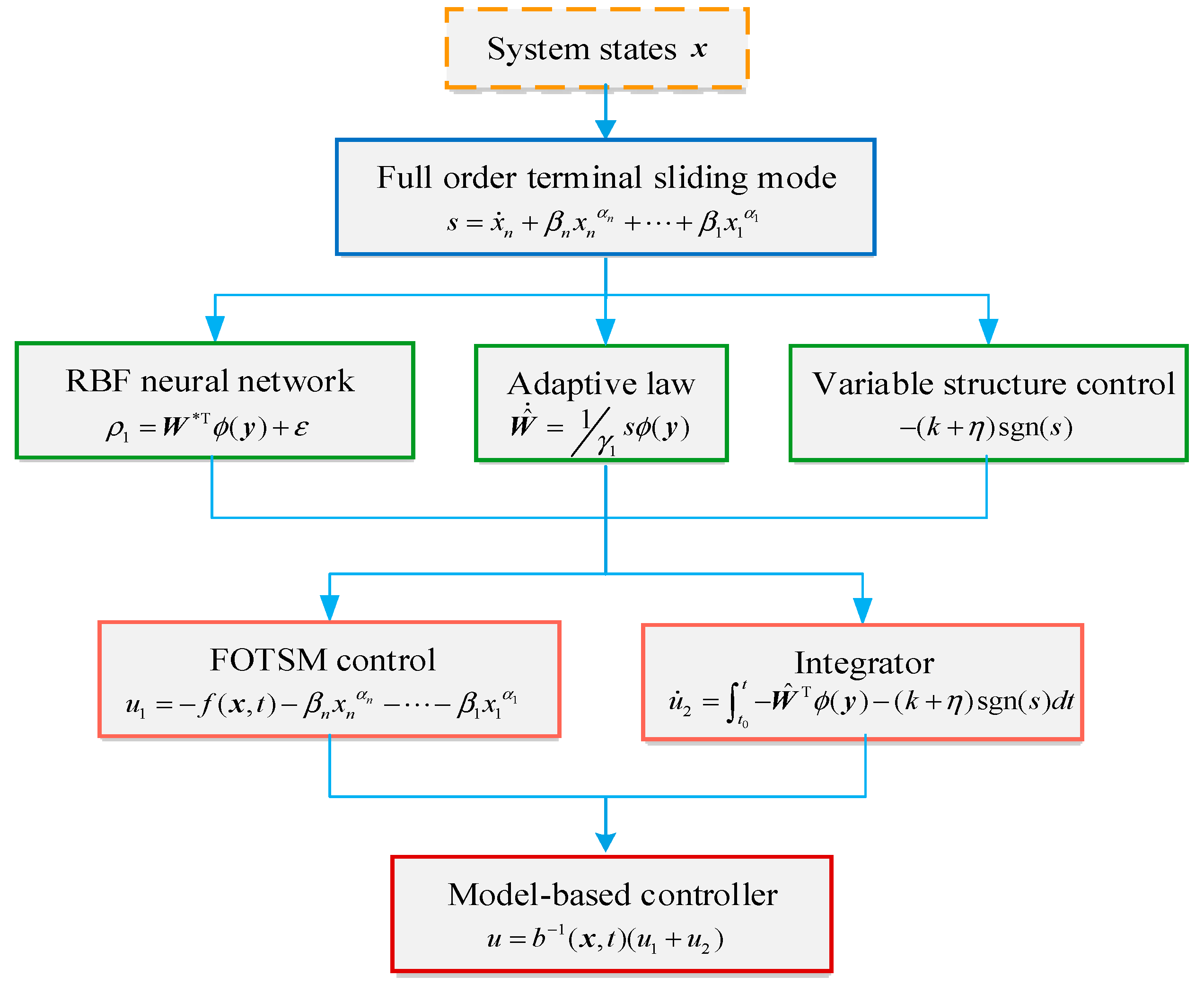
To sum up, the design procedures of the proposed model-based controller can be formulated by the block diagram of
Figure 1.
Theorem 1. Consider the nonlinear system given by Equation (1). If the controllers are designed as Equations (2) and (6)–(9), then the system state is bounded.
Proof. Design a Lyapunov function candidate as
where
.
Differentiating
with respect to time yields:
Substituting Equation (1) into Equation (2), we have
From Equations (6) and (7), it can be obtained that
Then, the time derivative of the FOTSM manifold is
According to Equations (4) and (8), rewrite the above equation as
Substituting Equations (9) and (15) into Equation (11) yields
Since
and
, it can be obtained that
According to Equations (10) and (17),
and
are bounded. From Definition 1 and the TSM control theory [
20,
25], the boundedness of the system state can also be ensured.
Since
, and
, then there is [
24]
Thus, is bounded. □
Theorem 2. For the nonlinear system expressed by Equation (1) and the controllers given by Equations (2) and (6)–(9), if in Equation (9) is designed so that, then the system is finite-time stable.
Proof. Design a Lyapunov function candidate as
Using Equations (6)–(8) and (12)–(15), we have
Since
and
, it can be obtained that
Therefore,
can be established [
20,
25]. Then from Remark 1, the system is finite-time stable. □
Remark 2. Equation (8) adopts the form of an integrator. Although the signum function is employed in it, the real control signal is continuous due to the effect of the integrator. Therefore, the chattering can be eliminated. Moreover, the designed controller avoids using the derivative of , which prevents the singularity from occurring.
Remark 3. It is noted that in some nonlinear systems, an integrator is more difficult to implement than a low-pass filter. Thus, in the next section, we will design a FOTSM controller using the form of low-pass filter.
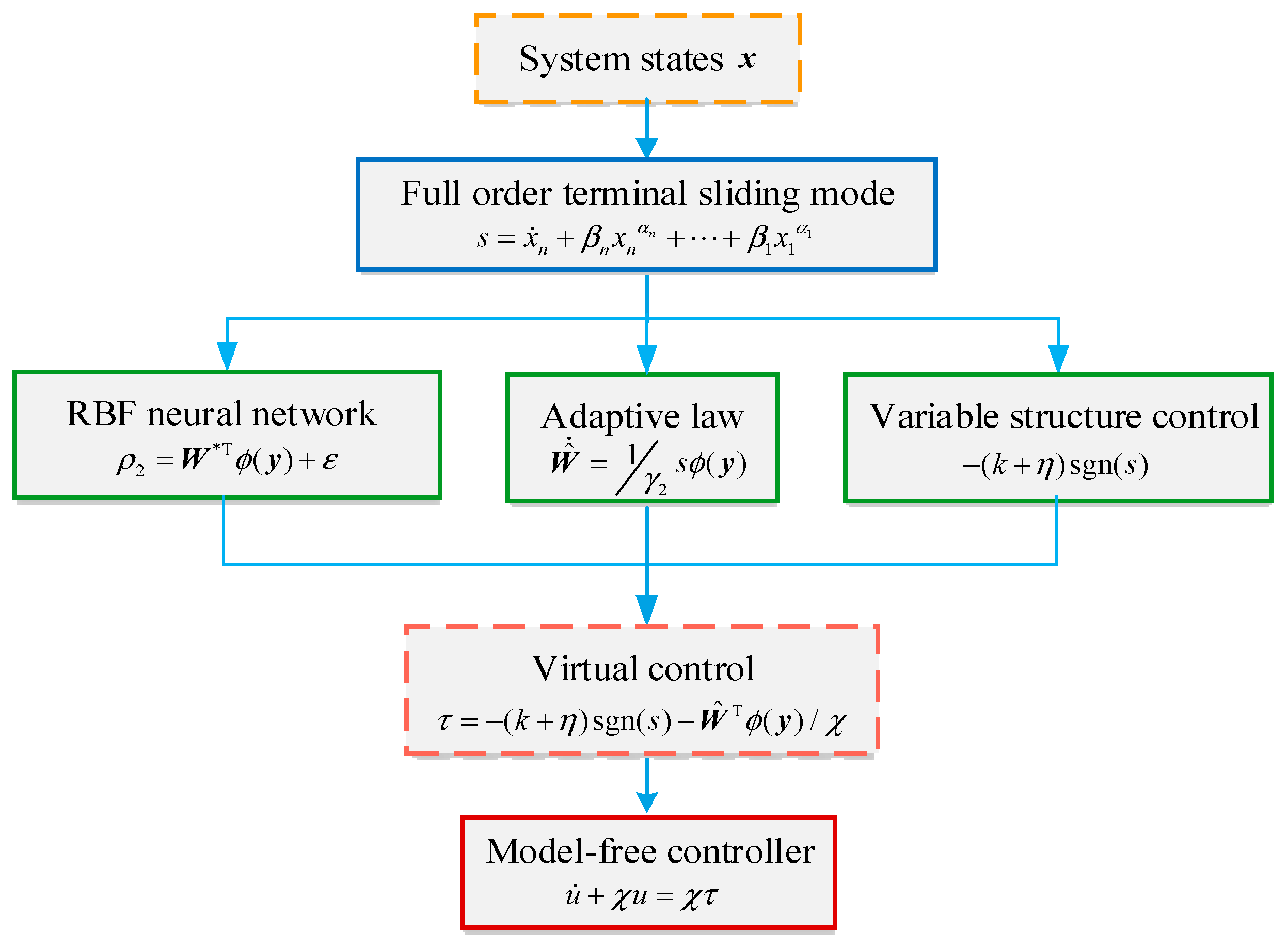
4. Model-Free FOTSM Controller
For the system in which neither
nor
is known, based on the RBF neural network, an adaptive FOTSM controller is further designed in this section by only using the system state; that is, it is like a model-free controller. To start, we rewrite Equation (1) as
where
.
The following assumption is given on the nonlinear system described by Equation (22).
Assumption 2. is Lipschitz continuous and positive; that is,, where. Moreover, is also Lipschitz continuous.
Remark 4. The above assumption is reasonable and does not lose generality, for many mechanical engineering systems fulfill this assumption, such as the robotic manipulator [6,15] and the spacecraft [7,8,9]. The controller is designed as
in which
,
stands for the virtual control input which will be determined later.
From Equations (22) and (23), one can figure out that
According to Equations (2) and (24), it can be obtained that
where
Similarly, we utilize the RBF network to estimate
; that is,
where
,
, and the other parameters are defined in Equations (4) and (5).
Then, the virtual control input
can be designed as
where
and
,
is updated as
where
.
To sum up, the design procedures of the proposed model-free controller can be formulated by the block diagram of
Figure 2.
Theorem 3. Consider the nonlinear system expressed by Equation (22). If the controllers are given by Equations (2), (23), (28), and (29), then the system state is bounded.
Proof. Design a Lyapunov function candidate as
Since
, it can be obtained that
.
Substituting Equations (9) and (25)–(28) into Equation (31) yields
Since
and
, it can be obtained that
Thus, as in
Section 3,
and
are bounded and the boundedness of the system state is also ensured. □
Theorem 4. Consider the nonlinear system expressed by Equation (22) and the controllers given by Equations (23), (28), and (29). If is designed so that, then the system state vector will converge to zero in finite time.
Proof. Design a Lyapunov function candidate as
Using Equations (22)–(29), we have
Since
and
, it can be obtained that
Therefore,
can be established according to the TSM control theory [
20,
25]. Then, from Remark 1, the system is finite-time stable. □
Remark 5. Equation (23) can smooth the control signal. Therefore, the chattering is attenuated.
Remark 6. If the powers are designed as, Equation (2) will become a full-order linear sliding mode. In that case, the designed controller still enables the avoidance of chattering while making the system state asymptotically converge.
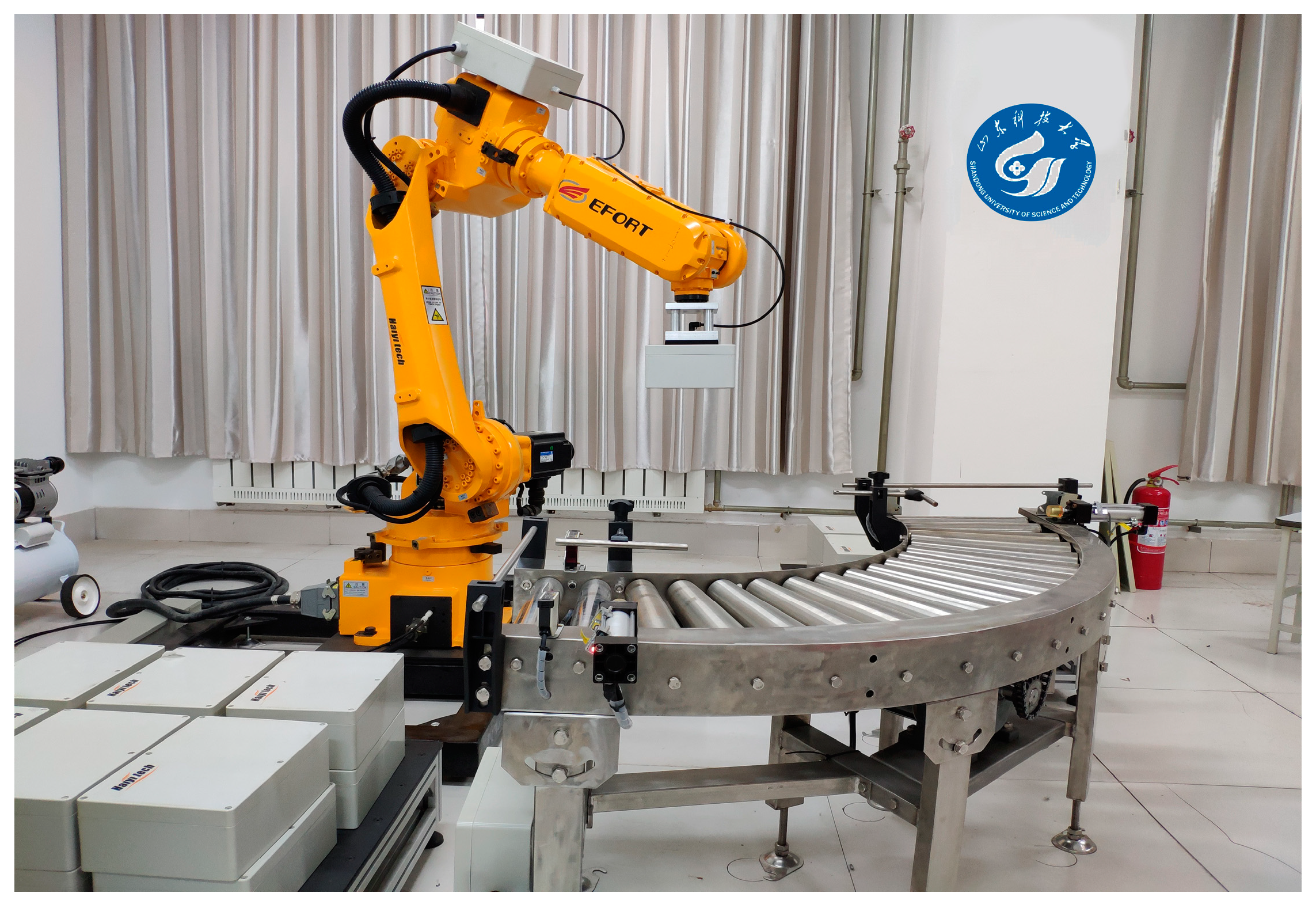
Remark 7. The proposed control concept can be used for many mechanical engineering systems, such as the multiple joint robotic manipulator shown in Figure 3. Its dynamic model can be described as a high-order nonlinear system. In the presence of dynamic uncertainties, the proposed control methods can be used to drive the joints to track the desired trajectories even when the dynamic model is not obtained. The RBF neural network can online estimate the dynamic model to enhance the control performance. Also, the tracking control is finite-time convergent, nonsingular, and chattering free. Thus, the proposed control methods can extend the application range of FOTSM to engineering systems. 5. Simulation Studies
This section shows how the designed controllers were applied to numerical system models to demonstrate their effectiveness. The numerical models and the simulation procedures exactly followed the literature [
20], but more uncertainties were introduced into the model parameters. All simulations were implemented on a laptop computer with an Intel Core i5-8250U CPU.
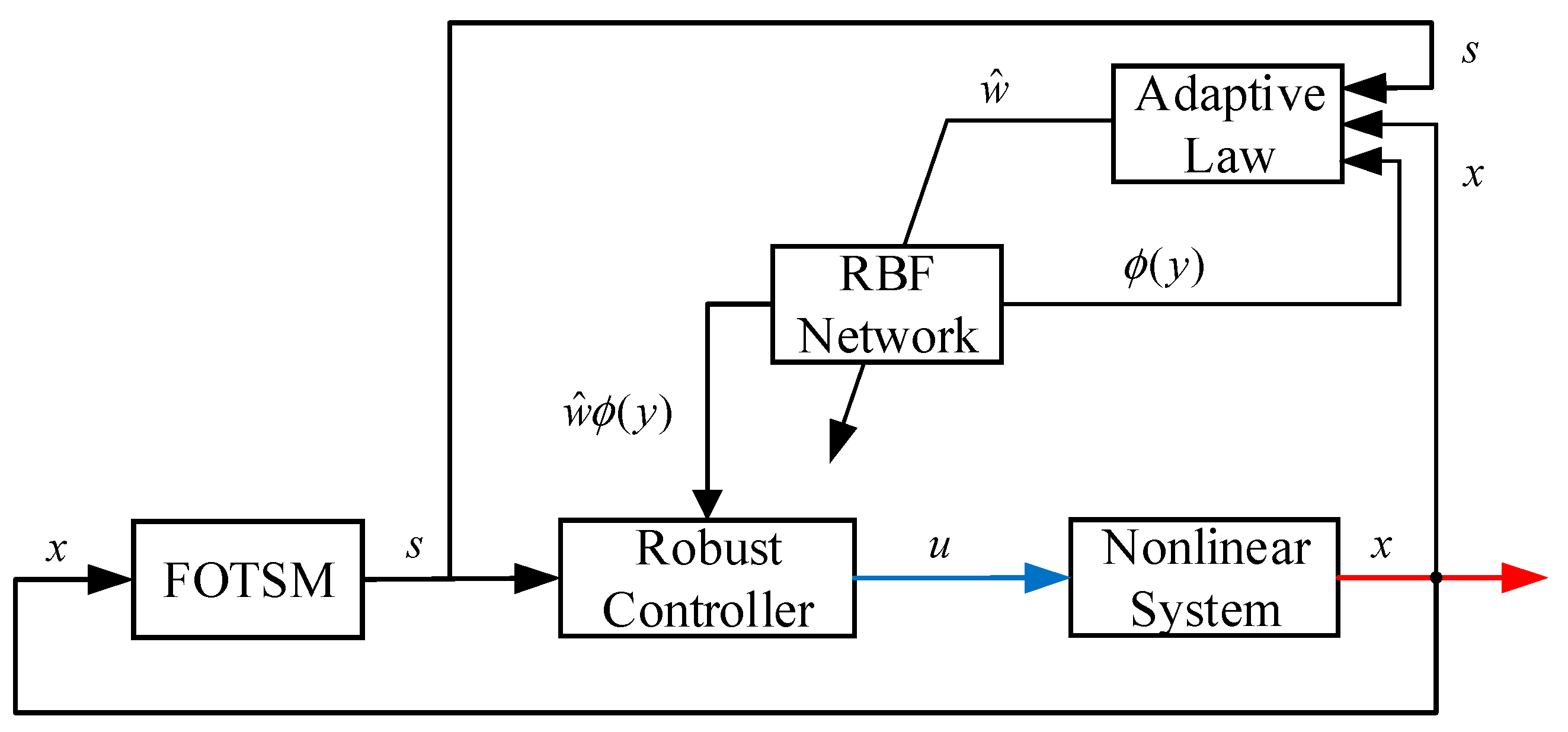
Figure 4 displays the simulation block diagram.
In the above block diagram, the control input
was constructed based on the FOTSM and RBF neural network and then applied to the nonlinear system. All the effort aimed at making the system state
converge to zero, which stands for that, in some mechanical engineering systems, the tracking error converges to zero. Similar to [
20], the simulation studies were formulated with second- and third-order systems, respectively.
5.1. Control of a Second-Order System
Here, we applied the designed schemes to a second-order system to verify their effectiveness. Two simulation cases are presented: the first case was a test of the model-based FOTSM controller, and the second case was a test of the model-free FOTSM controller.
The system model [
20] was
where
,
, and
,
.
Case 1. The test of the model-based FOTSM controller for the second-order nonlinear system.
In this case, the parameters are given in
Table 1.
The results are given in
Figure 5 and
Figure 6.
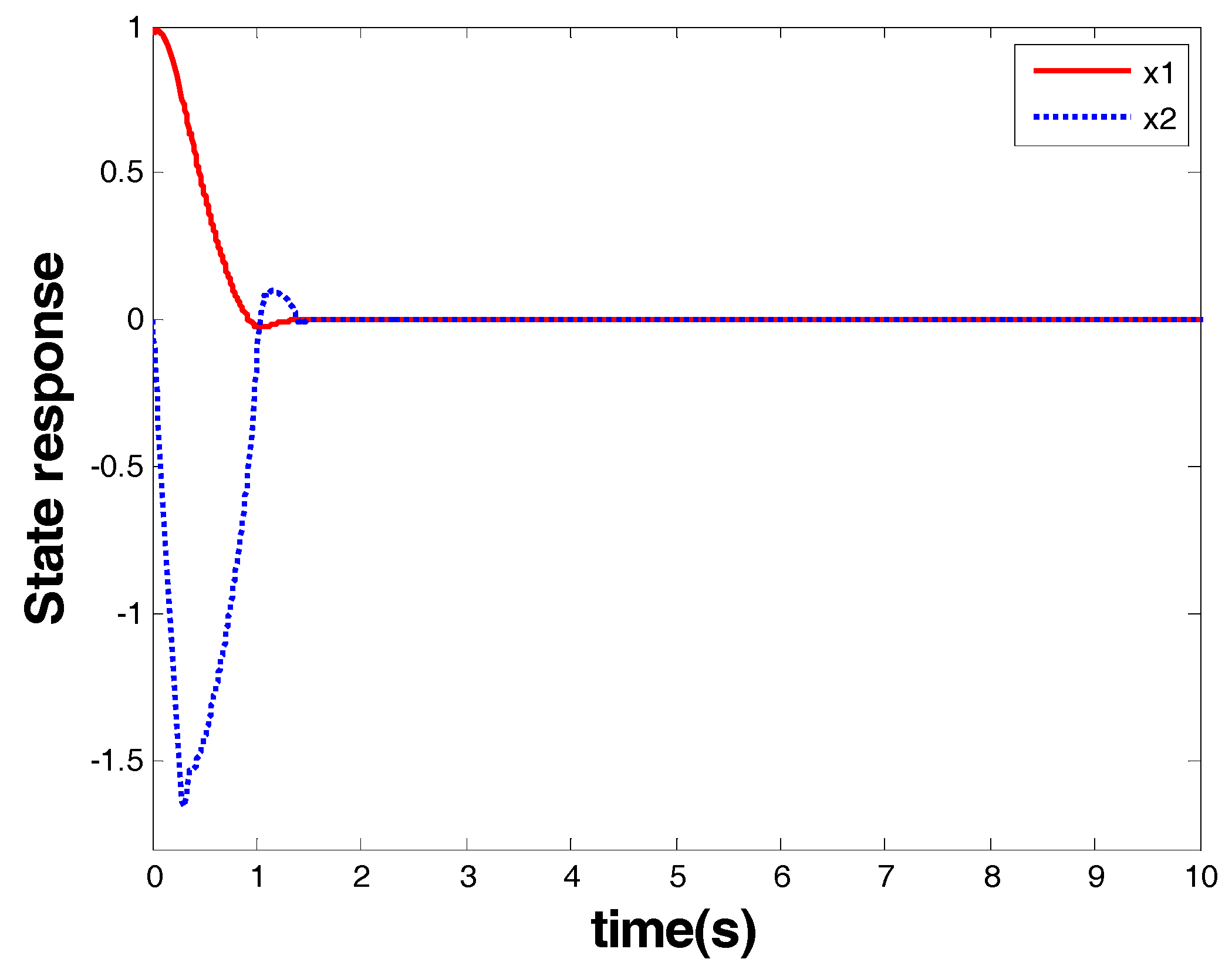
Figure 5 shows the response of the system state that is marked as a red arrow in
Figure 4.
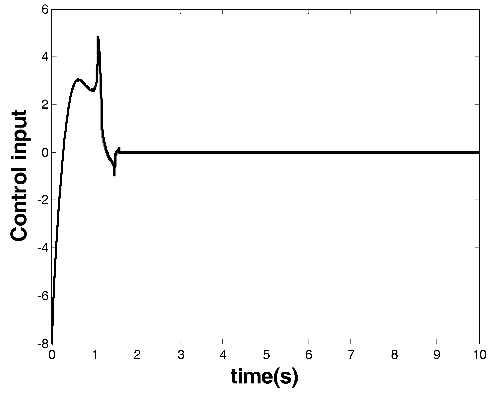
Figure 6 shows the control input that is marked as a blue arrow in
Figure 4. From the response of the system state and the controller, one can see that finite-time stability was ensured within 1.8 s by the model-based FOTSM controller. When the system state arrived at the origin, it stayed there even in the presence of uncertainties and disturbance. This demonstrates the robustness of the designed controller. Meanwhile, singularity and chattering problems did not occur, which shows the superior performance of the FOTSM control to overcome the two problems.
Case 2. The test of the model-free FOTSM controller for the second-order nonlinear system.
In this case, the parameters are given in
Table 2.
The results are given in
Figure 7 and
Figure 8.
Figure 7 shows the response of the system state that is marked as a red arrow in
Figure 4.
Figure 8 shows the control input that is marked as a blue arrow in
Figure 4. From the response of the system state and the controller, one can see that, similar to the model-based controller in last case, finite-time stability was also ensured by the model-free FOTSM controller. The advantage of the proposed controller over the existing robust FOTSM control methods was also verified, since the existing methods require a priori knowledge of the system model, while the proposed scheme does not.
5.2. Control of a Third-Order System
Here, we applied the designed schemes to a third-order system to verify their effectiveness. Similar to
Section 5.1, two tests are presented: one is for the model-based FOTSM controller, and the other is for the model-free FOTSM controller.
The system model [
20] was
where
,
, and the initial states of
,
and
are 1, −1, 0.
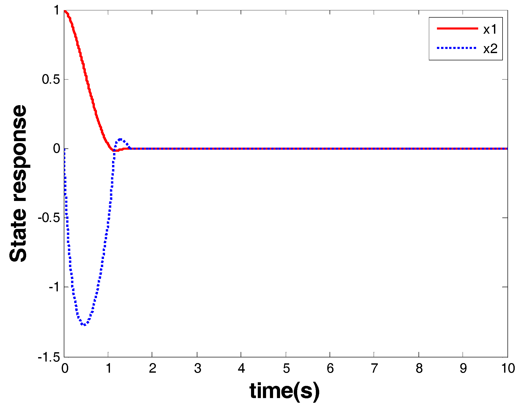
Case 3. The test of the model-based FOTSM controller for the third-order nonlinear system.
The parameters are given in
Table 3.
The results are given in
Figure 9 and
Figure 10.
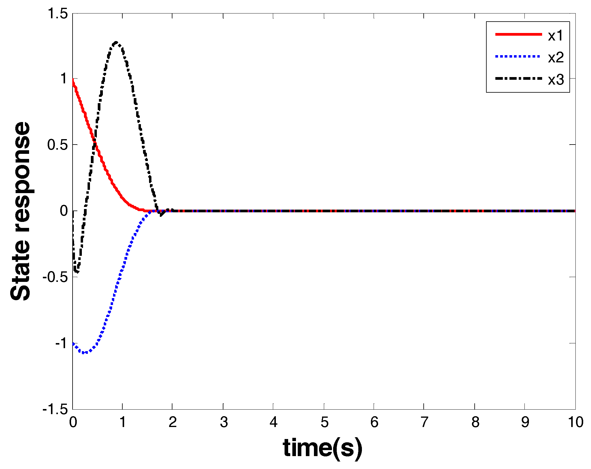
Figure 9 shows the response of the system state that is marked as a red arrow in
Figure 4.
Figure 10 shows the control input that is marked as a blue arrow in
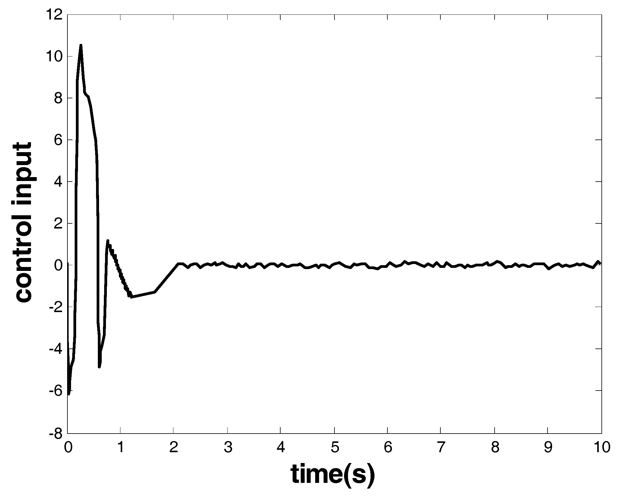
Figure 4. From the response of the system state and the controller, one can see that finite-time stability was ensured together with a chattering-free and nonsingular control performance. The convergence time was within 2.1 s, and the controller had robust performance against uncertainties.
Case 4. The test of the model-free FOTSM controller for the third-order nonlinear system.
In this case, the parameters were selected as and . The other parameters were chosen as in Case 3.
The results are given by
Figure 11 and
Figure 12.
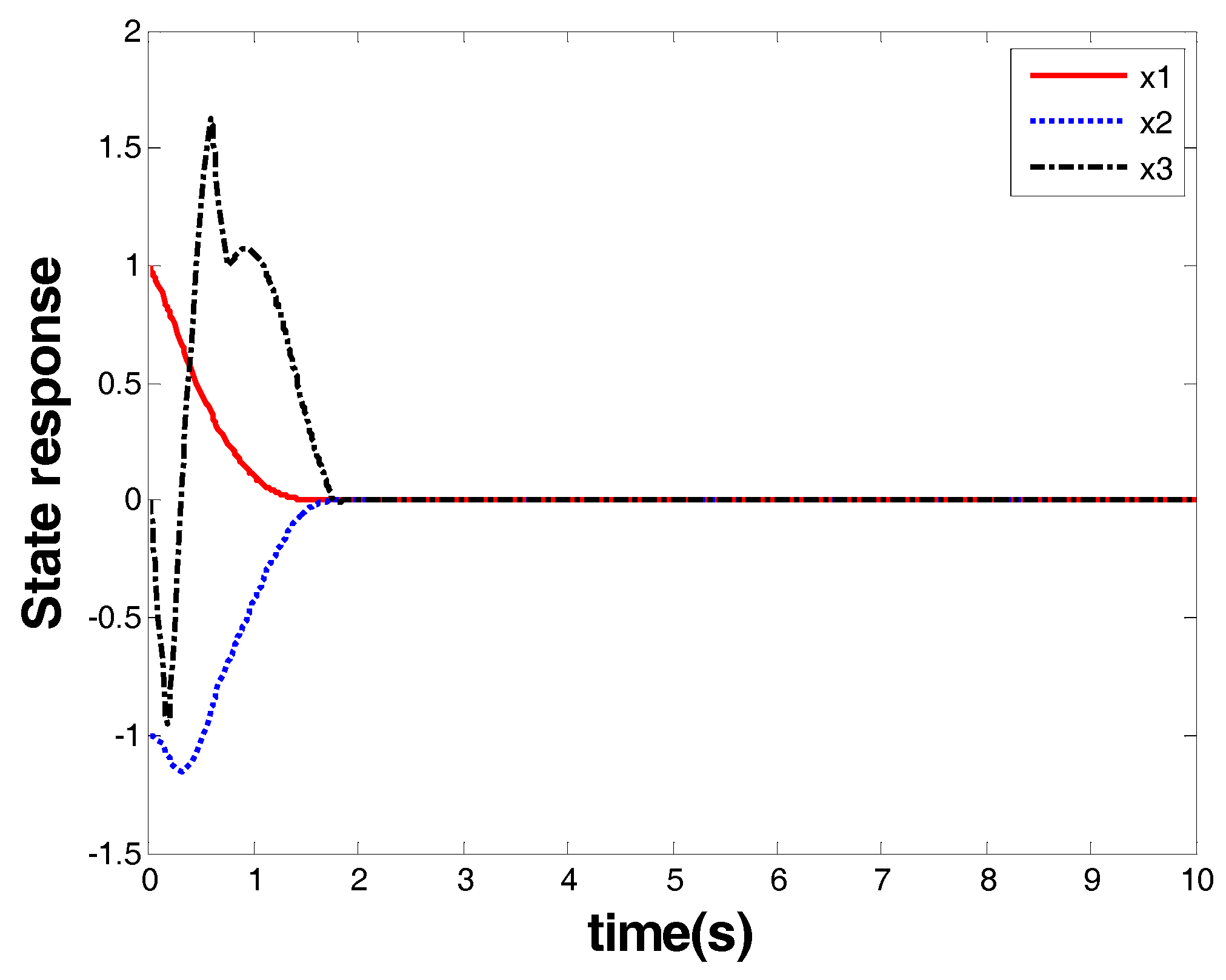
Figure 11 shows the response of the system state that is marked as a red arrow in
Figure 4.
Figure 12 shows the control input that is marked as a blue arrow in
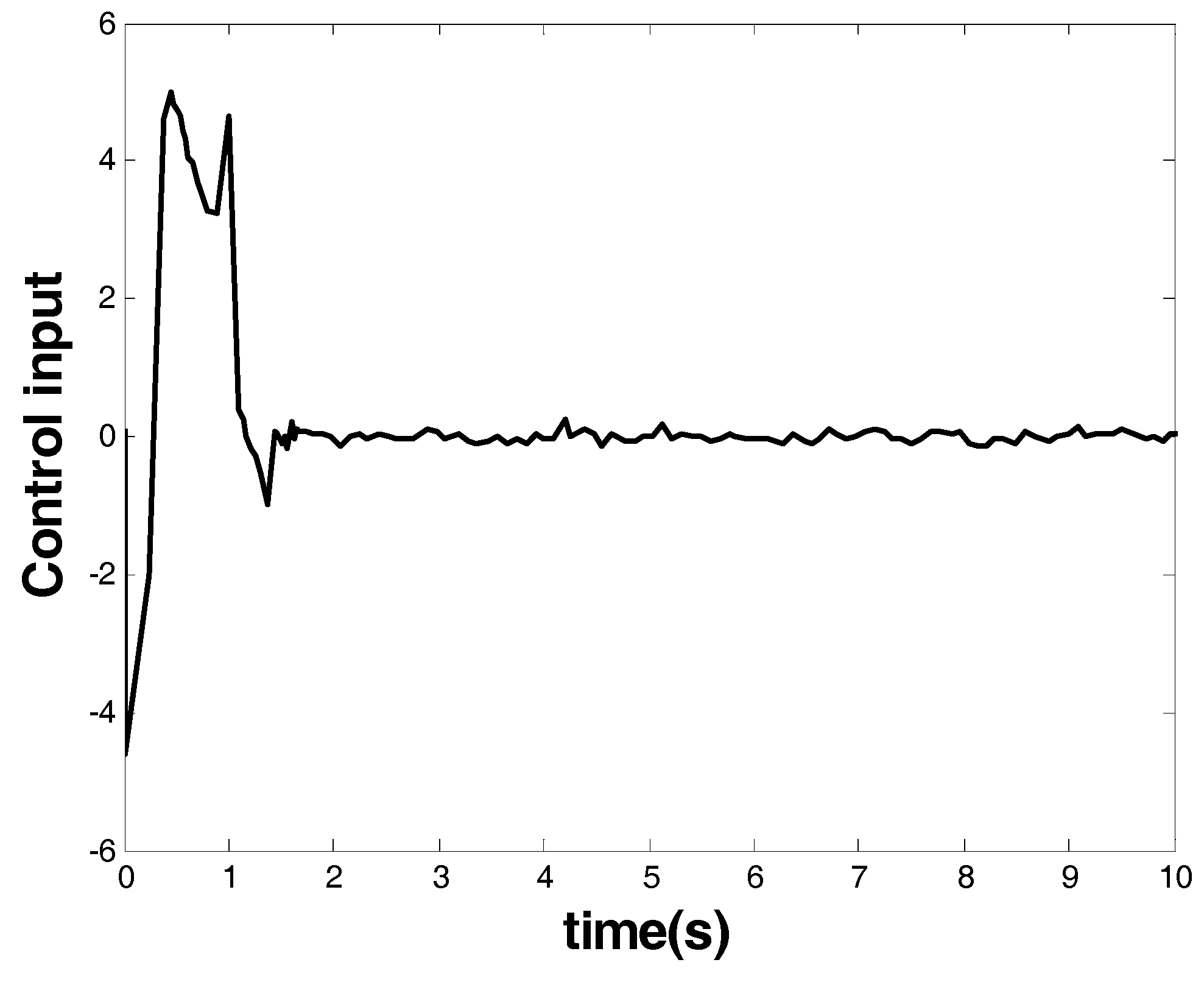
Figure 4. From the figures, one can see that the proposed model-free FOTSM controller also enabled the occurrence of finite-time convergence and achieved the attenuation of chattering and singularity. Therefore, this case verified the effectiveness of the model-free FOTSM controller for the third-order system.
6. Conclusions
The FOTSM control problem was investigated in this paper for high-order systems with modeling uncertainties. Two novel neural-network-based FOTSM control schemes were developed, which could achieve finite-time stability of high-order nonlinear systems. The designed schemes could essentially overcome the chattering and singularity problems.
The originality lies in that, unlike the existing FOTSM control methods, the designed control schemes need less information of the system model and the bounds of uncertainties’ derivatives. Thus, they can meet the needs of more application scenarios, especially when the information of the system model is difficult to obtain.
The designed controllers are for general high-order nonlinear systems. Thus, many industrial systems described by high-order nonlinear systems, such as n-link robotic manipulators, can utilize the proposed control concept in this paper to achieve finite-time convergent, nonsingular, and chattering-free feedback control performance.


