Image Feature Matching Based on Semantic Fusion Description and Spatial Consistency

Abstract

Image feature description and matching is widely used in computer vision, such as camera pose estimation. Traditional feature descriptions lack the semantic and spatial information, and give rise to a large number of feature mismatches. In order to improve the accuracy of image feature matching, a feature description and matching method, based on local semantic information fusion and feature spatial consistency, is proposed in this paper. Once object detection is used on images, feature points are then extracted, and image patches with various sizes surrounding these points are clipped. These patches are sent into the Siamese convolution network to get their semantic vectors. Then, semantic fusion description of feature points is obtained by weighted sum of the semantic vectors, and their weights optimized by particle swarm optimization (PSO) algorithm. When matching these feature points using their descriptions, feature spatial consistency is calculated based on the spatial consistency of matched objects, and the orientation and distance constraint of adjacent points within matched objects. With the description and matching method, the feature points are matched accurately and effectively. Our experiment results showed the efficiency of our methods.

1. Introduction

Image feature description and matching is the basic work of many tasks in image processing, such as image mosaic, camera pose estimation, 3D reconstruction, etc. The focus of this work is the extraction and description of image features. Up to now, researchers have carried out a lot of research on image feature extraction and description, and have produced many classic feature description and extraction methods, such as SIFT (scale-invariant feature transform) [1], SURF (speeded up robust features) [2], ORB (oriented FAST and rotated BRIEF) [3], and FAST (features from accelerated segment test) [4]. These methods obtain image feature points and their descriptors by searching the local extremum in the image, and describe the features using the luminance information of their neighborhood. Feature matching is obtained by way of calculating the distances between feature points in different images. For example, the SIFT feature descriptor uses Euclidean distance as the judgment standard between descriptors, while the BRIEF (binary robust independent elementary feature) descriptor [5] is a kind of binary descriptor, and hamming distance is used as the judgment standard to describe the correspondence of two feature points.

Recent years, convolution neural network has achieved remarkable results in the image processing. Through training, it can learn the semantic information from local image patches and object targets to the whole image. It has great advantages in image processing, such as object classification, detection, and semantic segmentation. In this paper, the convolution neural network is used as the component of the Siamese network [6] to deal with the different scales of neighborhood regions of image features, send the neighborhood image patches of different scales into the Siamese network branches, and obtain the description vectors with different scales of features. Through the normalized weight coefficient of these vectors, the feature description vectors with different scale information and robustness to the changes of illumination and rotation are obtained, and the matching relation between feature points is obtained by calculating the Euclidean distance of feature vectors.

Feature matching aims to find the correct corresponding points between images, whose focus is to confirm the accuracy of matching and remove mismatch. In this paper, we propose a feature-matching method based on feature spatial consistency. With object detection, images are separated into different object spaces (background is also regarded as an object), then we can track objects between images, and divide feature points into different spaces based on object spaces they belong to. For feature points, the matching space consistency is obtained by the object tracking results. Meanwhile, the feature points in one object space are connected as undigraph, which contains the spatial constraint in object spaces. We define the matching space consistency and the spatial constraint of object undigraph as the feature spatial consistency when matching feature points. An overview of our method is shown in Figure 1.

2. Related Work

2.1. Image Feature Extraction and Description Methods

In computer vision, local features of images have achieved considerable success in many aspects, such as stereo vision, SFM (structure from motion), attitude estimation, classification, detection, medical imaging, etc. In the long-term study, researchers in the field of computer vision have designed many stable local image features, such as SIFT (scale-invariant feature transform) [1], Harris angle point [7], FAST (features from accelerated segment test) angle point [4], ORB (oriented FAST and rotated BRIEF) feature point [3], etc., all of which have the same properties, such as repeatability, distinguishability, efficiently, and locality. A vector describing information about the pixels around the key handcrafted points is a traditional feature point descriptor.

These traditional methods of feature point extraction and description are handcrafted, which only contains the local pixel gradient information around the feature point, lacks the image semantic information, and is vulnerable to the changes of illumination and rotation. That is, for images with repetitive structures and similar textures, the feature descriptors are highly similar and cannot be highly distinguished. Recent years, with the success of deep learning, some new feature extraction and description methods are emerged. For example, TILDE (Temporally Invariant Learned DEtector) [8] used the generalized hinging hyperplanes function as the object function to extract the feature points of a series of images of the same position, but this method only processes images of the same scene, and lacks universality. Karel Lenc [9] formulates feature detection as a regression problem, which tries to use powerful regressors, such as deep networks, to automatically learn which visual structures provide stable anchors for local feature detection, however, extracting features using regressors will lead to an inevitable increase in computing and time costs.

In the aspect of feature description, traditional methods describe features with vectors constructed by the gradient information of surrounding pixels, such as SIFT and BRIEF, which have difficulty distinguishing feature points with similar textures. Therefore, learning a function to discriminatively describe image patches around feature points as the description of feature becomes one popular idea at present, where the input is the context window of feature points, and the output vector is regarded as the description of feature points. Here, the function can be composed of several modules, such as order algorithm pool [10], boosting method [11], or CNN (convolution neural network) [12,13]. In these methods, fixed-size image patches (64 × 64) around feature points are clipped as objects to be handled, and obtain the semantic vectors of patches as description of feature points in the center of the patches with the functions learned. These methods, especially the method proposed in [12], have shown more excellent performance than traditional methods. However, using only a fixed size of image patches is not comprehensive, and may lose other useful information, in addition, the size of patches which is the most suitable is still not an established standard.

2.2. Feature-Matching Methods

In the aspect of matching accuracy judgment, methods based on probability inference [14,15] and methods based on graph [16,17,18,19] are two important kinds of methods at present. The former methods use a function to represent the mapping relationship between the matching feature points, and optimize function parameters by matching points in the dataset, and matching points which are not suited to the function are removed, while the latter methods connect the feature points as a graph. By using the connectivity of the graph, the matching of adjacent feature points is taken as the constraint condition to remove mismatch. All these two kinds of methods consider the matching of adjacent feature points, and can partly improve the accuracy of feature matching. However, these methods only use the feature description in feature matching—the global and local information of images is discarded, which are easily affected by other mismatches, and lead to lower accuracy.

2.3. Object Detection Methods

Object detection is a classical task in computer vision. In the past few decades, people have conducted a significant amount of research and produced a lot of methods. Before 2012, the idea of classification tasks in object detection was to train the shallow classifier to complete classification tasks by using the handcrafted features. Most non-textured object instance detection is based on template matching. The early template matching method [20,21] used the Chamfer distance to measure the difference between the template and the input image contour. Ref. [22] was based on the AdaBoost algorithm framework, by using the Haar-like wavelet portraiture classification, and the sliding window search strategy was adopted to achieve accurate and effective positioning. Ref. [23] proposed using the partial gradient direction histogram (HOG) of the image as a feature and use the SVM (support vector machine) as a classifier for pedestrian detection. Ref. [24] proposed the multi-scale deformation component model (DPM), one of the most influential methods of object category detection, which inherited the advantages of using HOG feature and SVM classifier. The DPM object detector consists of a root filter and some component filters, and uses the sliding window strategy to search the target in different scale and aspect ratio images. The advantages of these traditional target detection methods are that they do not require a large amount of labeling data, but the disadvantages are that they have lower precision/recall ratios and accuracy.

In 2012, Ref. [25] proposed the image classification algorithm of deep convolutional neural network (DCNN) based on deep learning theory, which greatly improved the accuracy of image classification. Since then, the deep convolutional neural network has developed rapidly in the field of object detection. At present, object detection methods based on deep learning mainly fall into two directions: (1) The method based on region proposal (two stages) mainly includes R-CNN (region-based convolutional neural networks) [26], Fast R-CNN [27], Faster R-CNN [28], R-FCN (region-based fully convolutional network) [29], etc., which first produces region proposals by RPN (region proposal networks), and then classifies them. (2) Regressive methods (single-stage), such as SSD (single shot multi-box detector) [30], YOLO (you only look once) [31], DSSD (deconvolutional single shot detector) [32], etc., use the idea of regression. Given the input image, the object bounding box and object category of this box are directly predicted in multiple positions of the image.

3. Feature Description Method Based on Semantic Fusion

3.1. Object Detection on Images

Before feature extraction and description, object detection is firstly used as preprocessing on images being processed, in order to obtain the object information. In this paper, we choose the pre-trained SSD (single shot multi-box detector) object detection algorithm.

SSD algorithm is one of the major object detection frameworks at present, which is proposed by Wei Liu on ECCV 2016. It has an obvious speed advantage over Faster R-CNN [28] and mAP advantage over YOLO [31]. SSD inherited the idea of transforming detection into regression from YOLO, and completed object location and classification at one time. Meanwhile, based on anchor in faster RCNN, it proposed a detection method based on a similar prior box, and added a detection method based on pyramidal feature hierarchy, that is, predicting the object on feature maps of different sensory fields. The schematic is shown in Figure 2.

3.2. ORB Feature Extraction

Feature points are extracted after object detection so that the object labels of all feature points can be obtained. Here, we choose ORB [3], which is defined by the luminance of their neighbor pixels as our candidate feature, as shown in Figure 3. In contrast to SIFT [1], SURF [2], and other feature extraction methods, ORB feature is more real-time, and takes into account certain accuracy and robustness.

ORB feature is based on FAST feature points [4], and contains additional orientation and scale information. ORB feature has on scale invariability, by building scale pyramid and detecting angular points on each layer, while the orientation of ORB feature is calculated by gray centroid method, that is, connecting the geometric center $O$ and mass center $C$ of image patch as vector $\overrightarrow{OC}$, the orientation of feature points is calculated by image moment

$$\theta =\arctan \left(m_{01}/m_{10}\right).$$

(1)

The moment of image patch is $m_{pq}={\displaystyle \sum _{x,y\in B}{x}^p{y}^{q}I(x,y),p,q=\left\{0,1\right\}}$, and $C=\left(\frac{m_{10}}{m_{00}},\frac{m_{01}}{m_{00}}\right)$.

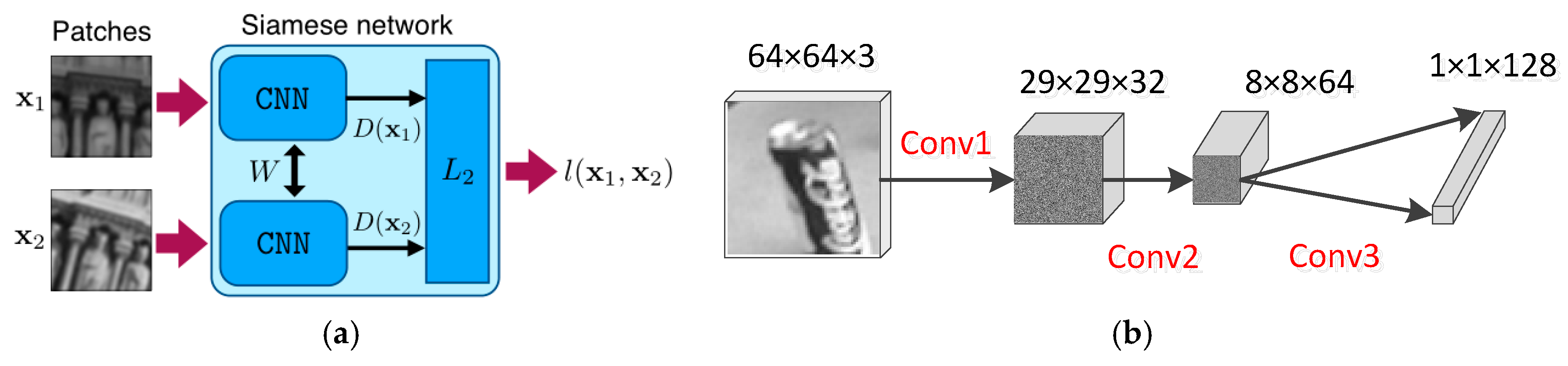
3.3. Semantic Fusion Description of Feature Point Based on Siamese Network

Inspired by the feature description methods of [12,13], in this paper, we propose a semantic fusion description method of feature aims to take full advantage of local semantic information around feature points. Thus, semantic information of different sizes of image patches around the feature points will be fused into the feature point descriptions to enhance the robustness of feature descriptions.

Specifically, after feature extraction, image patches of size 8 × 8, 16 × 16, 32 × 32, 64 × 64 around feature points are clipped, and resized to 64 × 64 as the inputs of a trained convolutional neural network, in order to generate the semantic descriptions of these patches. Then, we assign different weights to every semantic description, and add them together as our semantic fusion description of the feature. The weights assigned these descriptions are finally optimized by the PSO (particle swarm optimization) algorithm.

In this paper, we choose the Siamese network used in [12] to generate the patch semantic descriptions, which composed of two convolutional neural networks (CNN) branches with shared weights. When training the Siamese network, pairs of image patches in different images are sent into two CNN branches, respectively, and obtain the output descriptions, by maximizing (minimizing) the L2 distances of the descriptions of (non-)corresponding image patches around feature points, the parameters of the net can finally learn how to discriminatively describe image patches. After training, the semantic descriptions of image patches can be obtained by sending into the CNN branch. The architecture of the Siamese network is shown in Figure 4.

Based on the above calculation results, and the object labels of feature points obtained in Section 3.1, we can finally obtain the semantic fusion descriptions of feature, which contains both the local and object semantic information. Our description is written as

$$\begin{array}{cc}\hfill R_m^c& =a_1·R_{8\times 8}+a_2·R_{16\times 16}+a_3·R_{32\times 32}+a_4·R_{64\times 64}\hfill \\ \hfill & =a_1·CN{N}_{Siamese}\left(I_{8\times 8}\right)+a_2·CN{N}_{Siamese}\left(I_{16\times 16}\right)+a_3·CN{N}_{Siamese}\left(I_{32\times 32}\right)\hfill \\ \hfill & +a_4·CN{N}_{Siamese}\left(I_{64\times 64}\right)\hfill \end{array}$$

(2)

where $I_{n\times n},n=8,16,32,64$ means the size of image patches. $a_1,a_2,a_3,a_4$ as the normalized weights, and $a_1+a_2+a_3+a_4=1$, $CN{N}_{Siamese}(•)$ means the generating of semantic descriptions of patches by the CNN branch of the Siamese network, $c$ means the object label of the feature point which is obtained in Section 3.1. The schematic of our method is showed in Figure 5.

3.4. Weights Optimization Based on PSO

The values of $a_1,a_2,a_3,a_4$ are optimized by PSO algorithm. We use the Oxford affine covariant features dataset [33] as our training data, which contains a series of sequence images and has been given the homographic matrix $H$ between of any two images in each sequence. Then, suppose there are two images $I_i$ and $I_j$ to be processed, the objective function to be optimized is

$$E_R=\min ({\displaystyle \sum _{i=1}^n{D}_{i,j}}),$$

(3)

where $D_{i,j}$ means the distance between two matching feature points in $I_i$ and $I_j$, and is defined as

$$D_{i,j}={\Vert \left(R_i-R_j\right)\Vert }_2=\sqrt{{\displaystyle {\sum }_{\begin{array}{l}n=8,16,32,64\\ i=1,2,3,4\end{array}}{\left(a_i·R_{n\times n}^i-a_i·R_{n\times n}^j\right)}^2}}.$$

(4)

$R_{n\times n}^i,R_{n\times n}^j$ means a pair of matching feature points in $I_i$ and $I_j$. The optimization algorithm steps are written as follows:

• Initialize $X_k=\left[{a_1}^k,{a_2}^k,{a_3}^k,{a_4}^k\right],k=1,2,\cdots 100$ randomly in range of [0,1] as particle swarm, which is satisfied with $a_1^k+a_2^k+a_3^k+a_4^k=1$.
• For all these particles, $pbest$ means their historical optimal values, which are initialized by the initial values of particles, $gbest$ means the global optimal value of the particle swarm.
• The objection function is written as

  $$\begin{array}{cc}\hfill E_R& =E=\min ({\displaystyle \sum _{\begin{array}{l}x=1\\ y=1\end{array}}^N{\Vert R_x-R_y\Vert }_2})\hfill \\ \hfill & =\min ({{\displaystyle \sum _{z=1}^n\Vert \left(a_1·R_8^x+a_2·R_{16}^x+a_3·R_{32}^x+a_4·R_{64}^x\right)-\left(a_1·R_8^y+a_2·R_{16}^y+a_3·R_{32}^y+a_4·R_{64}^y\right)\Vert }}_2).\hfill \end{array}$$

  (5)
• Define the iteration as 1000 and, for every iteration, the speed and locations of particles will be updated as

  $$\{\begin{array}{c}{v}_{m+1}=v_m+c_1\times rand()\times \left(pbes{t}_m-x_m\right)+c_2\times rand()\times \left(gbes{t}_m-x_m\right)\\ x_{m+1}=x_m+v_m\end{array}.$$

  (6)

  where $v_m$ and $x_m$ means the speed and location of a particle in the m-th iteration, $v_{m+1}$ and $x_{m+1}$ means the updated speed and location in the next iteration, $rand()$ means the random number between 0 and 1.

4. Feature-Matching Algorithm Based on Feature Spatial Consistency

Feature spatial consistency means the spatial mapping relation of feature between different images. Due to the wide distribution of feature points in images, it is not realistic to seek the spatial consistency of discrete feature points directly. Obviously, it is easy to obtain object spatial consistency as objects contain more semantic and spatial information than feature points, and the feature spatial consistency could be obtained between the consistent object spaces. Following this idea, we obtain feature spatial consistency through two steps, firstly, obtain the spatial consistency of objects, which shrinks the rough spatial consistency from image level to object level; secondly, obtain the distance and orientation constraints of other points in the corresponding object spaces, which shrinks the feature spatial consistency from of object level to level of local image patch, which is inside object spaces.

Therefore, images to be processed are first divided into different object spaces based on object detection, so feature points are assigned to object spaces which they are included. The object spatial consistency is obtained by object tracking using L-K (Lucas-Kanade) optical flow [34], then, for feature points in every object space, feature spatial consistency is finally obtained by combining the object spatial consistency and the orientation and distance constraints within the object space together.

4.1. Object Spatial Consistency Based on SSD

For images $I_i$ and $I_j$ to be processed, as object detection is done on them in Section 3.1, they are then separated into different object spaces (background is also regarded as a kind of object). The object detection results can be formulized as $ROI{s}_m=CNN\left(I_m\right),m=i,j$, where $I_m$ means $I_i$ and $I_j$, $ROI{s}_m$ means the results of object detection on $I_i$ and $I_j$, i.e., the spatial positions of objects in $I_i$ and $I_j$.

Then the object spatial consistency can be obtained by tracking objects between images $I_i$ and $I_j$ based on object detection results. Specifically, by using the L-K optical flow [34], we can get the approximate transform matrix H between $I_i$ and $I_j$, which can be used to calculate the reprojection of points from $I_i$ to $I_j$. For instance, suppose there is an object on $I_i$, and we got the vertexes of space bounding box of $ob{j}_i$ by object detection, clockwise defined as (x_A,y_A),(x_B,y_B),(x_C,y_C),(x_D,y_D), then the relocation coordinate of the vertexes in $I_j$, $\left(x_A^{\prime },y_A^{\prime }\right),\left(x_B^{\prime },y_B^{\prime }\right),\left(x_C^{\prime },y_C^{\prime }\right),\left(x_D^{\prime },y_D^{\prime }\right)$, are calculated by

$$\left[\begin{array}{c}{x}_n^{\prime }\\ y_n^{\prime }\\ 1\end{array}\right]=H•\left[\begin{array}{c}{x}_n\\ y_n\\ 1\end{array}\right],$$

(7)

where $n=A,B,C,D$, and the left side of the equation means the reprojection coordinates of the vertexes in $I_j$.

According to Formula (5), we can calculate the area of $ob{j}_j$ bounding box $S_{ob{j}_i}$ and its reprojection box area $S_{ob{j}_i}^{\prime }$ in $I_j$ with the following two formulas:

$$S_{obj}=\left(\max \left(x_B,x_D\right)-\min \left(x_A,x_C\right)\right)\times \left(\max \left(y_C,y_D\right)-\min \left(y_A,y_B\right)\right),$$

(8)

$$S_{obj}^{\prime }=\left(\max \left(x_B^{\prime },x_D^{\prime }\right)-\min \left(x_A^{\prime },x_C^{\prime }\right)\right)\times \left(\max \left(y_C^{\prime },y_D^{\prime }\right)-\min \left(y_A^{\prime },y_B^{\prime }\right)\right).$$

(9)

The coordinates of the mass center $\left(x_{mass},y_{mass}\right)$ in the reprojection box can be obtained by

$$\{\begin{array}{c}{x}_{mass}=\frac{1}{2}\times \left(\max \left(x_B^{\prime },x_D^{\prime }\right)-\min \left(x_A^{\prime },x_C^{\prime }\right)\right)\\ y_{mass}=\frac{1}{2}\times \left(\max \left(y_B^{\prime },y_D^{\prime }\right)-\min \left(y_A^{\prime },y_C^{\prime }\right)\right)\end{array}.$$

(10)

Suppose there are n objects ($ob{j}_j^n,n=1,2,\dots$) detected on $I_j$, which belong to the same object kind as $ob{j}_i$, and the areas of their bounding boxes are calculated by Formula (6), then the $IoU$ ratios between the areas of these boxes and $S_{ob{j}_i}^{\prime }$ is

$$IoU=\frac{S_{ob{j}_i}^{\prime }\cap S_{ob{j}_j^n}}{S_{ob{j}_i}^{\prime }\cup S_{ob{j}_j^n}},n=1,2,\dots n.$$

(11)

Thus, there will be n pairs of corresponding objects. In all of the objects pairs, the object which owns the max $IoU$ ratio and the min distance of mass centers with the reprojection box is regarded as the correct corresponding object of $ob{j}_i$ in $I_j$. Therefore, for every object in $I_i$, we can track it in $I_j$ based on the above formulas, and constitute the set of corresponding objects $C_{object}=\left\{\frac{S_{ob{j}_i^1}}{S_{ob{j}_j^1}}=s_1,\frac{S_{ob{j}_i^2}}{S_{ob{j}_j^2}}=s_2,\cdots ,\frac{S_{ob{j}_i^n}}{S_{ob{j}_j^n}}=s_n\right\}$, $s_n\left(n=1,2,\cdots n\right)$ means the $IoU$ ratio of a pair of corresponding object areas.

In this way, we could obtain the object spatial consistency of all objects between $I_i$ and $I_j$, as Figure 6 shows.

4.2. Distance and Orientation Constraints within Object Spaces

Based on the object spatial consistency obtained above, the distance and orientation constraints of feature points within each object space are defined as follows.

According to the set, $C_{object}$, constituted by corresponding objects between $I_i$ and $I_j$, we can connect points in the corresponding object spaces as undigraph using Delaunay triangulation as shown in Figure 7.

Suppose there is a feature point $v_i$ in $ob{j}_i^1$ in $I_i$, $V_i=\left\{v_1^i,v_2^i,\cdots ,v_n^i\right\}$ means the set of adjacent points of $v_i$, $v_j$ means the matching point of $v_i$ in $ob{j}_j^1$ in $I_j$, and $V_j=\left\{v_1^j,v_2^j,\cdots ,v_n^j\right\}$ means the set constituted by the matching points of elements in $V_i$. The distance constraint and orientation constraints which are described as follows.

• The distance constraint. On the basis of the correspondence of $V_i$ and $V_j$, we can construct a set of relative distances $D_{V_i,V_j}=\left\{d_{v_1^i,v_1^j},d_{v_2^i,v_2^j},\cdots ,d_{v_n^i,v_n^j}\right\}$, the elements in the set are the relative distances between the points in $V_i$ and their corresponding points in $V_j$:

  $$d_{v_a^i,v_a^j}=\sqrt{{\left(x_a^i-x_a^j\right)}^2+{\left(y_a^i-y_a^j\right)}^2},a=1,2,\dots ,n,$$

  (12)

  and the relative distance between $v_i$ and $v_j$, which is signed as $d_{v_i,v_j}$, should satisfy the constraint that $d_{v_i,v_j}\in \left[\min \left(D_{V_i,V_j}\right),\max \left(D_{V_i,V_j}\right)\right]$, $\min \left(D_{V_i,V_j}\right)$ and $\max \left(D_{V_i,V_j}\right)$ mean the minimum and maximum of $D_{V_i,V_j}$.
• The orientation constraint. Calculate the orientation vectors of $V_i$ and $V_j$, signed as and constructed as a set $K_{V_i,V_j}=\left\{k_{v_1^i,v_1^j},k_{v_2^i,v_2^j},\cdots ,k_{v_n^i,v_n^j}\right\}$, the element in the set is written as:

  $$k_{{v^{\prime }}_a^i,v_a^i}=\frac{y_{v_a^j}-y_{v_a^i}}{x_{v_a^j}-x_{v_a^i}},a=1,2,\dots ,n,$$

  (13)

  and the orientation vector between $v_i$ and $v_j$, which is signed as $k_{v_i,v_j}=\frac{y_{v_j}-y_{v_i}}{x_{v_j}-x_{v_i}}$, should satisfy the constraint that $k_{v_i,v_j}\in \left[\min \left(K_{V_i,V_j}\right),\max \left(K_{V_i,V_j}\right)\right]$. The example is shown in Figure 8.

Thus, the feature spatial consistency is finally constructed by the object consistency and the interactive distance and orientation constraints in object spaces, and only matching points which are coincide the feature spatial consistency will be reserved in the process of feature matching.

4.3. Feature Matching with Feature Spatial Consistency

Based on the matching method described above with feature spatial consistency, feature points will be matched in two steps. Firstly, we calculate their matching points by L2 distances of their semantic fusion descriptions. For all pairs of matching points, only pairs of matching points whose object labels are the same are reserved.

Then, for the remaining pairs of matching points whose object labels are the same, we construct undigraph in every object space with feature points which are in the same space using Delaunay triangulation. Then, for vertex points in every undigraph, the correctness of the matching between them and their corresponding points are estimated by the distance and orientation constraints of their adjacent points.

Thus, with the two steps above, matching points which coincide with the feature spatial consistency will be reserved. On the contrary, matching points which do not coincide with feature spatial consistency will be removed. The test results of our matching method are shown in Section 5.

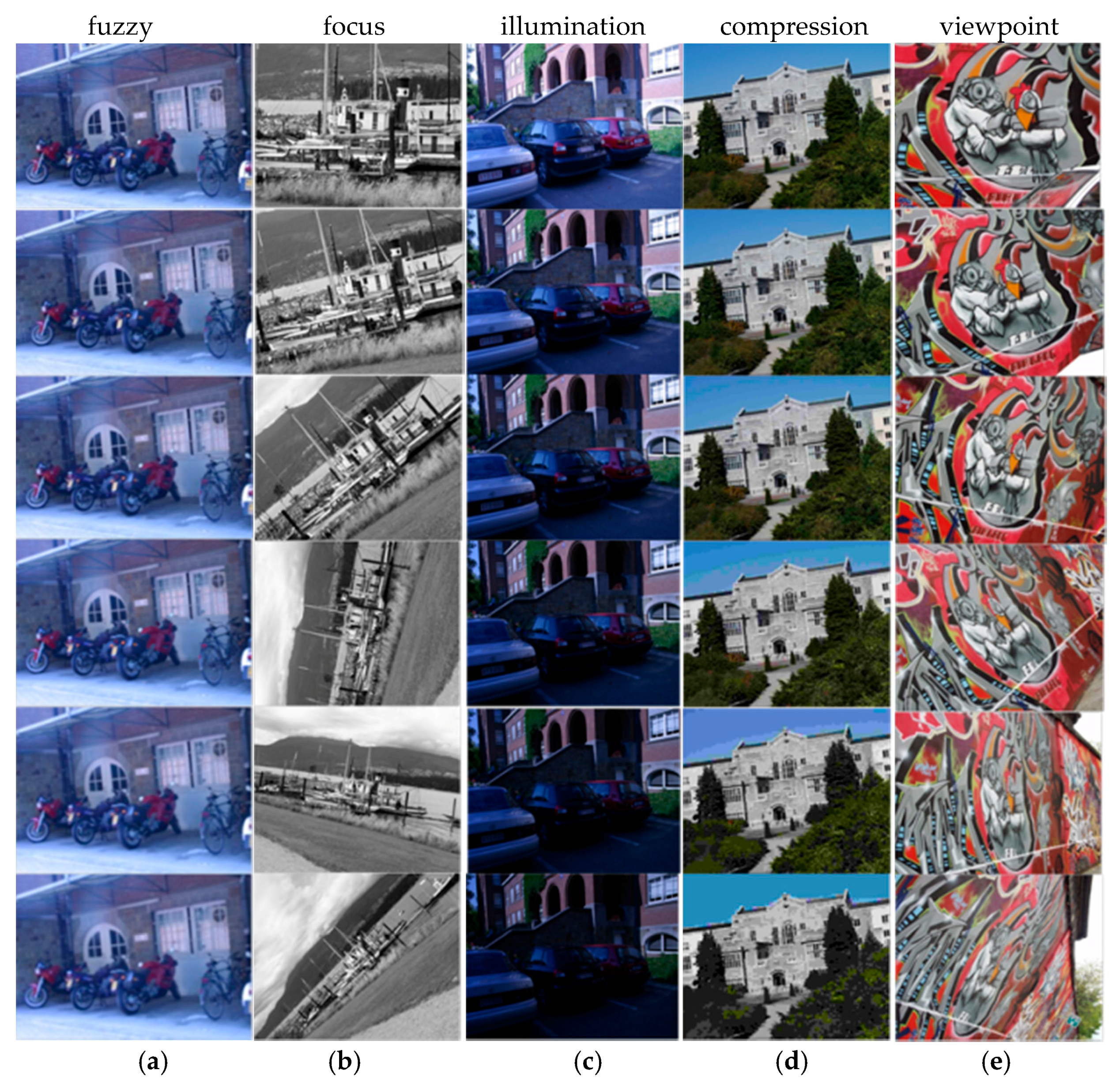
5. Experiment Design and Result Analysis

5.1. Parameters Optimization of Feature Semantic Description

The parameters of semantic fusion feature description, proposed in Section 3.3, are optimized using PSO algorithm on the affine covariant features dataset [33], which has several sequences of images with several kinds of conversion, e.g., fuzzy transformation, focus transform, viewpoint changing, illumination, and compression changes. In every sequence, the homography matrix between any two images is given as the ground truth. The example images are shown in Figure 9.

When training the parameters, we selected several sequences images in the dataset, extract the ORB feature points in every image and obtain their description with our method, and the parameters in the description are assigned randomly between 0 and 1 before training. Then, the feature points are matched between any two images, and we select the correct matching based the ground truth homography matrix. All the L2 distances between matching feature will be added up as the ${\displaystyle \sum _{i=1}^n{D}_{i,j}}$, which need to be minimized in Formula (3), and then we can obtain the trained parameters. The correctness curve of total L2 distances of feature in every training epoch is shown in Figure 10.

The parameters after optimization are tested in two sequences: bikes and bark. We chose the L2 distances between feature vectors ranking from the min to the max as the thresholds to calculate the precision and recall from 0 to 1. We test our method with other feature descriptions, such as ORB + BRIEF, SIFT, and the method in [12], and draw the PR (Precision-Recall) curve and count the AUC (area under curve) of these curves in Figure 11 and

Table 1. AUC of curves in bikes and bark sequences.

AUC	ORB + BRIEF	SIFT	Method in [12]	Ours
bikes sequence	0.58	0.62	0.71	0.79
bark sequence	0.47	0.71	0.68	0.77

. The results in Figure 11 and Table 1 show that our semantic fusion description of feature achieves the higher accuracy in test images.

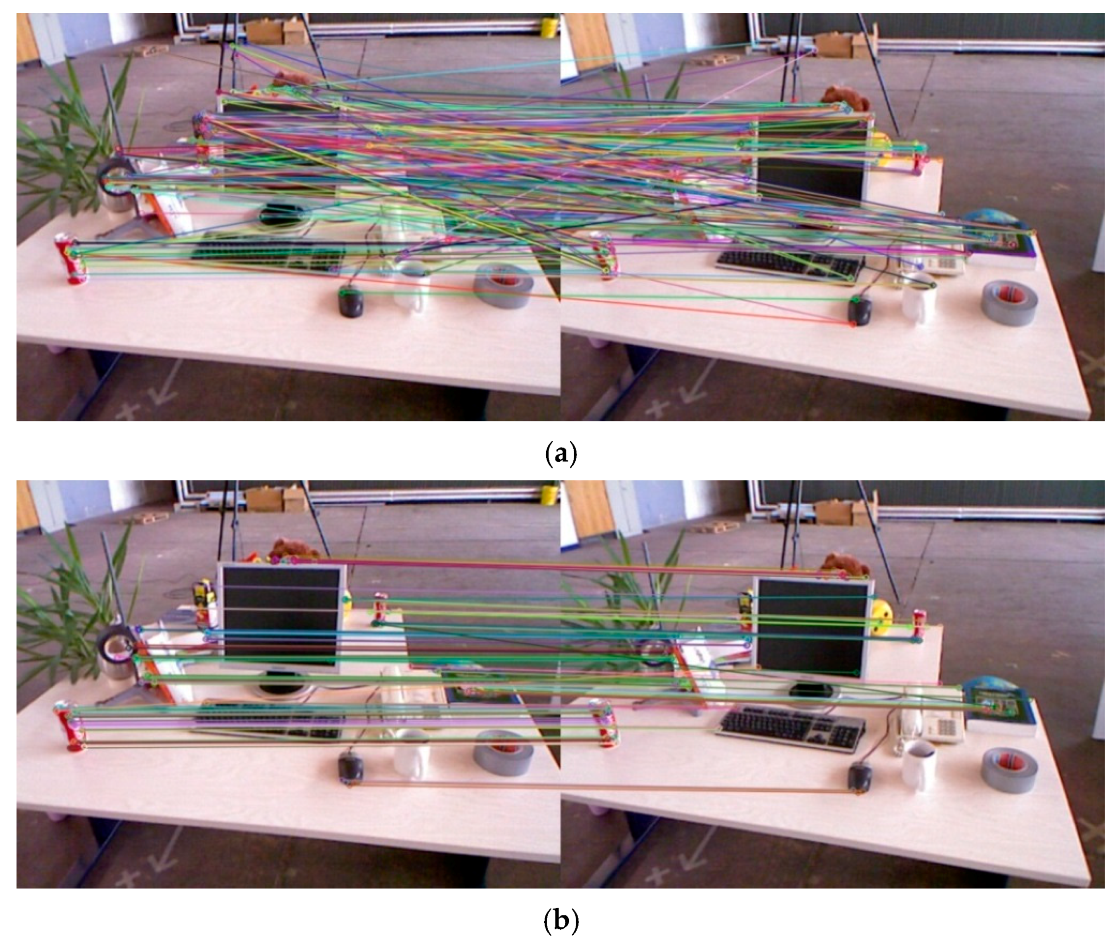
5.2. Feature Matching and Mismatch Removal

We choose the TUM dataset [35] to test our feature-matching method described in Section 4. The TUM indoor dataset contains a continuous sequence of images and provides the standard track and realistic camera pose files, which are useful to our test experiments.

We select three feature extraction and description methods which are widely used, and our feature description method to test our feature-matching method. When doing the experiment, we test our feature-matching method on several descriptions, such as ORB+BRIEF, SIFT, description proposed in [12], and our feature description method, and compare the original matching results and the final results of these feature descriptions. We drew the PR curves before and after using our matching method and, in addition, we count the AUC of these curves, and the results are shown as Figure 12 and

Table 2. AUC of the matching results in Figure 12.

AUC	SIFT	ORB + BRIEF	Method in [12]	Our Method
Before mismatch removal	0.65	0.60	0.69	0.73
After mismatches removal	0.72	0.67	0.79	0.82

.

The results in Table 2 show that our feature-matching method can also effectively optimize the results of other feature-matching methods, which means our method has a certain degree of universality. This can also be verified by Figure 13 and Figure 14.

All of our experiments are run on a computer with two Titan XP GPUs. The time of computing the feature semantic fusion descriptions of an image is close to 100 ms. For our feature-matching method, in order to obtain the global optimal matching, every feature point needs to participate in calculations n times, thus, the time complexity of our feature method is O(n²).

6. Conclusions

In this paper, we proposed a semantic fusion description of feature points, and a method of feature matching based on feature spatial consistency. We use a Siamese network to obtain the semantic vectors of image patches around feature points, and fused these semantic vectors together as the descriptions of feature points centered in the patches. Then, we match the feature points using feature spatial consistency combined by object spatial consistency and distance orientation constraints within object spaces. The results of experiments demonstrate that our semantic fusion descriptions of features are more accurate and robust, and our feature-matching method can efficiently improve the accuracy of matching results. In the future, we will try to improve our network and reduce the time complexity of our feature-matching method.

References

1. Lowe, D.G. Distinctive Image Features from Scale-Invariant Keypoints. Int. J. Comput. Vis. 2004, 60, 91–110. [Google Scholar] [CrossRef] [Green Version]
2. Bay, H.; Tuytelaars, T.; Gool, L.J.V. SURF: Speeded Up Robust Features. In Proceedings of the 9th European Conference on Computer Vision, Graz, Austria, 7–13 May 2006; Part I. pp. 404–417. [Google Scholar] [CrossRef]
3. Rublee, E.; Rabaud, V.; Konolige, K.; Bradski, G.R. ORB: An efficient alternative to SIFT or SURF. In Proceedings of the IEEE International Conference on Computer Vision, ICCV 2011, Barcelona, Spain, 6–13 November 2011; pp. 2564–2571. [Google Scholar] [CrossRef]
4. Rosten, E.; Drummond, T. Machine Learning for High-Speed Corner Detection. In Proceedings of the Computer Vision-ECCV2006, 9th European Conference on Computer Vision, Graz, Austria, 7–13 May 2006; Part I. pp. 430–443. [Google Scholar] [CrossRef]
5. Calonder, M.; Lepetit, V.; Strecha, C.; Fua, P. BRIEF: Binary Robust Independent Elementary Features. In Proceedings of the Computer Vision-ECCV 2010, 11th European Conference on Computer Vision, Heraklion, Crete, Greece, 5–11 September 2010; Part IV. pp. 778–792. [Google Scholar] [CrossRef]
6. Bromley, J.; Bentz, J.W.; Bottou, L.; Guyon, I.; LeCun, Y.; Moore, C.; Säckinger, E.; Shah, R. Signature Verification Using A “Siamese” Time Delay Neural Network. IJPRAI 1993, 7, 669–688. [Google Scholar] [CrossRef]
7. Harris, C.G.; Stephens, M. A Combined Corner and Edge Detector. In Proceedings of the Alvey Vision Conference, AVC 1988, Manchester, UK, 31 August–2 September 1988; pp. 1–6. [Google Scholar] [CrossRef]
8. Verdie, Y.; Yi, K.M.; Fua, P.; Lepetit, V. TILDE: A Temporally Invariant Learned DEtector. In Proceedings of the IEEE Conference on Computer Vision and Pattern Recognition, CVPR 2015, Boston, MA, USA, 7–12 June 2015; pp. 5279–5288. [Google Scholar] [CrossRef]
9. Lenc, K.; Vedaldi, A. Learning Covariant Feature Detectors. In Proceedings of the Computer Vision-ECCV 2016 Workshops, Amsterdam, The Netherlands, 8–10 and 15–16 October 2016; Part III. pp. 100–117. [Google Scholar] [CrossRef]
10. Brown, M.A.; Hua, G.; Winder, S.A.J. Discriminative Learning of Local Image Descriptors. IEEE Trans. Pattern Anal. Mach. Intell. 2011, 33, 43–57. [Google Scholar] [CrossRef] [PubMed] [Green Version]
11. Trzcinski, T.; Christoudias, C.M.; Lepetit, V. Learning Image Descriptors with Boosting. IEEE Trans. Pattern Anal. Mach. Intell. 2015, 37, 597–610. [Google Scholar] [CrossRef] [PubMed] [Green Version]
12. Simo-Serra, E.; Trulls, E.; Ferraz, L.; Kokkinos, I.; Fua, P.; Moreno-Noguer, F. Discriminative Learning of Deep Convolutional Feature Point Descriptors. In Proceedings of the 2015 IEEE International Conference on Computer Vision, ICCV 2015, Santiago, Chile, 7–13 December 2015; pp. 118–126. [Google Scholar] [CrossRef]
13. Zbontar, J.; LeCun, Y. Stereo Matching by Training a Convolutional Neural Network to Compare Image Patches. J. Mach. Learn. Res. 2016, 17, 2. [Google Scholar]
14. Fischler, M.A.; Bolles, R.C. Random Sample Consensus: A Paradigm for Model Fitting with Applications to Image Analysis and Automated Cartography. Commun. ACM 1981, 24, 381–395. [Google Scholar] [CrossRef]
15. Chen, J.; Ma, J.; Yang, C.; Tian, J. Mismatch removal via coherent spatial relations. J. Electron. Imaging 2014, 23, 043012. [Google Scholar] [CrossRef]
16. Caetano, T.S.; Caelli, T.; Schuurmans, D.; Barone, D.A.C. Graphical Models and Point Pattern Matching. IEEE Trans. Pattern Anal. Mach. Intell. 2006, 28, 1646–1663. [Google Scholar] [CrossRef] [PubMed]
17. Caetano, T.S.; McAuley, J.J.; Cheng, L.; Le, Q.V.; Smola, A.J. Learning Graph Matching. IEEE Trans. Pattern Anal. Mach. Intell. 2009, 31, 1048–1058. [Google Scholar] [CrossRef] [PubMed]
18. Cho, M.; Alahari, K.; Ponce, J. Learning Graphs to Match. In Proceedings of the IEEE International Conference on Computer Vision, ICCV 2013, Sydney, Australia, 1–8 December 2013; pp. 25–32. [Google Scholar] [CrossRef]
19. Cho, M.; Sun, J.; Duchenne, O.; Ponce, J. Finding Matches in a Haystack: A Max-Pooling Strategy for Graph Matching in the Presence of Outliers. In Proceedings of the 2014 IEEE Conference on Computer Vision and Pattern Recognition, CVPR 2014, Columbus, OH, USA, 23–28 June 2014; pp. 2091–2098. [Google Scholar] [CrossRef]
20. Olson, C.F.; Huttenlocher, D.P. Automatic target recognition by matching oriented edge pixels. IEEE Trans. Image Process. 1997, 6, 103–113. [Google Scholar] [CrossRef] [PubMed] [Green Version]
21. Gavrila, D.; Philomin, V. Real-Time Object Detection for “Smart” Vehicles. In Proceedings of the Seventh IEEE International Conference on Computer Vision, Kerkyra, Greece, 20–27 September 1999; pp. 87–93. [Google Scholar] [CrossRef]
22. Viola, P.A.; Jones, M.J. Rapid Object Detection using a Boosted Cascade of Simple Features. In Proceedings of the 2001 IEEE Computer Society Conference on Computer Vision and Pattern Recognition (CVPR 2001), Kauai, HI, USA, 8–14 December 2001; pp. 511–518. [Google Scholar] [CrossRef]
23. Dalal, N.; Triggs, B. Histograms of Oriented Gradients for Human Detection. In Proceedings of the 2005 IEEE Computer Society Conference on Computer Vision and Pattern Recognition (CVPR 2005), San Diego, CA, USA, 20–26 June 2005; pp. 886–893. [Google Scholar] [CrossRef]
24. Forsyth, D.A. Object Detection with Discriminatively Trained Part-Based Models. IEEE Comput. 2014, 47, 6–7. [Google Scholar] [CrossRef]
25. Krizhevsky, A.; Sutskever, I.; Hinton, G.E. ImageNet Classification with Deep Convolutional Neural Networks. In Proceedings of the 26th Annual Conference on Neural Information Processing Systems 2012, Lake Tahoe, NV, USA, 3–6 December 2012; pp. 1106–1114. [Google Scholar]
26. Girshick, R.B.; Donahue, J.; Darrell, T.; Malik, J. Rich Feature Hierarchies for Accurate Object Detection and Semantic Segmentation. In Proceedings of the 2014 IEEE Conference on Computer Vision and Pattern Recognition, CVPR 2014, Columbus, OH, USA, 23–28 June 2014; pp. 580–587. [Google Scholar] [CrossRef]
27. Girshick, R.B. Fast R-CNN. In Proceedings of the 2015 IEEE International Conference on Computer Vision, ICCV 2015, Santiago, Chile, 7–13 December 2015; pp. 1440–1448. [Google Scholar] [CrossRef]
28. Ren, S.; He, K.; Girshick, R.B.; Sun, J. Faster R-CNN: Towards Real-Time Object Detection with Region Proposal Networks. In Proceedings of the Annual Conference on Neural Information Processing Systems 2015, Montreal, QC, Canada, 7–12 December 2015; pp. 91–99. [Google Scholar]
29. Dai, J.; Li, Y.; He, K.; Sun, J. R-FCN: Object Detection via Region-based Fully Convolutional Networks. In Proceedings of the Annual Conference on Neural Information Processing Systems 2016, Barcelona, Spain, 5–10 December 2016; pp. 379–387. [Google Scholar]
30. Liu, W.; Anguelov, D.; Erhan, D.; Szegedy, C.; Reed, S.E.; Fu, C.; Berg, A.C. SSD: Single Shot MultiBox Detector. In Proceedings of the Computer Vision-ECCV 2016-14th European Conference, Amsterdam, The Netherlands, 11–14 October 2016; Part I. pp. 21–37. [Google Scholar] [CrossRef]
31. Redmon, J.; Divvala, S.K.; Girshick, R.B.; Farhadi, A. You Only Look Once: Unified, Real-Time Object Detection. In Proceedings of the 2016 IEEE Conference on Computer Vision and Pattern Recognition, CVPR 2016, Las Vegas, NV, USA, 27–30 June 2016; pp. 779–788. [Google Scholar] [CrossRef]
32. Fu, C.; Liu, W.; Ranga, A.; Tyagi, A.; Berg, A.C. DSSD: Deconvolutional Single Shot Detector. arXiv, 2017; arXiv:1701.06659. [Google Scholar]
33. Affine Covariant Features Database for Evaluating Feature Detector and Descriptor Matching Quality and Repeatability. Available online: http://www.robots.ox.ac.uk/~vgg/research/affine (accessed on 15 July 2017).
34. Lucas, B.D.; Kanade, T. An Iterative Image Registration Technique with an Application to Stereo Vision. In Proceedings of the 7th International Joint Conference on Artificial Intelligence, IJCAI’81, Vancouver, BC, Canada, 24–28 August 1981; pp. 674–679. [Google Scholar]
35. A Benchmark for the Evaluation of RGB-D SLAM Systems. Available online: https://vision.in.tum.de/data/datasets/rgbd-dataset (accessed on 14 October 2017).
Figure 1. The pipeline of our method. For images to be processed, object detection method is first used to obtain the object information of images for the computing of feature spatial consistency, and the feature description is obtained by the Siamese network.
Symmetry 10 00725 g001
Figure 2. The single shot multi-box detector (SSD) algorithm schematic quoted from [30].
Symmetry 10 00725 g002
Figure 3. ORB feature point extracting based on the luminance of neighbor pixels.
Symmetry 10 00725 g003
Figure 4. Architecture of the Siamese network we use. (a) The global architecture of the Siamese network; (b) The architecture of CNN branch in the Siamese network, the filter sizes of Conv1, Conv2, and Conv3 layers are 7 × 7, 6 × 6, and 5 × 5.
Symmetry 10 00725 g004
Figure 5. The semantic fusion descriptions of feature points based on our method.
Symmetry 10 00725 g005
Figure 6. Obtain feature spatial consistency. For example, (a) means original image I i , which uses SSD for object detection; (b) means I j , and for the object “tv” detected in I i , its reprojection box is calculated in I j , which is drawn in black. The white box represents the same kind of object “tv” detected in I j , since the two boxes has the max I o U ratio, the two objects are regarded as the same one and constituted a corresponding object pair, that is, there is the object spatial consistency between the two “tv” spaces in I i and I j .
Symmetry 10 00725 g006
Figure 7. The instance of constructing undigraph of feature points in an object space. (a) The feature points extracted in an object space; (b) The undigraph connected by the remaining points whose matching points are in the same object spaces.
Symmetry 10 00725 g007
Figure 8. The constraints of distance and orientation in the undigraph of object spaces.
Symmetry 10 00725 g008
Figure 9. Examples of the affine covariant features dataset [33]. Images in sequences of (a), (b), (c), (d) and (e) contain conversions of fuzzy transformation, focus transform, illumination, compression changes and viewpoint changing respectively.
Symmetry 10 00725 g009
Figure 10. The total vector L2 distances of matching feature points in every training epoch.
Symmetry 10 00725 g010
Figure 11. PR (Precision-Recall) curves of weights optimization. (a) The results tested on bikes sequence; (b) The results tested on bark sequence.
Symmetry 10 00725 g011
Figure 12. PR curves of our matching method. (a) Matching results tested with SIFT; (b) Matching result tested with ORB and BRIEF; (c) Matching result tested with method in [12]; (d) Matching result tested with our method. Black curves mean the original matching results, the blue curves mean the final matching using our matching method.
Symmetry 10 00725 g012
Figure 13. Feature-matching results using our matching method with ORB + BRIEF. (a) The original matching results; (b) The results using our feature-matching method.
Symmetry 10 00725 g013
Figure 14. Feature-matching results using our matching method with ORB + our feature description. (a) The original matching results; (b) The results using our feature-matching method.
Symmetry 10 00725 g014