Generalized Modified Slash Birnbaum–Saunders Distribution


Abstract
:1. Introduction
1.1. Birnbaum–Saunders Distribution
1.2. Slash Methodology
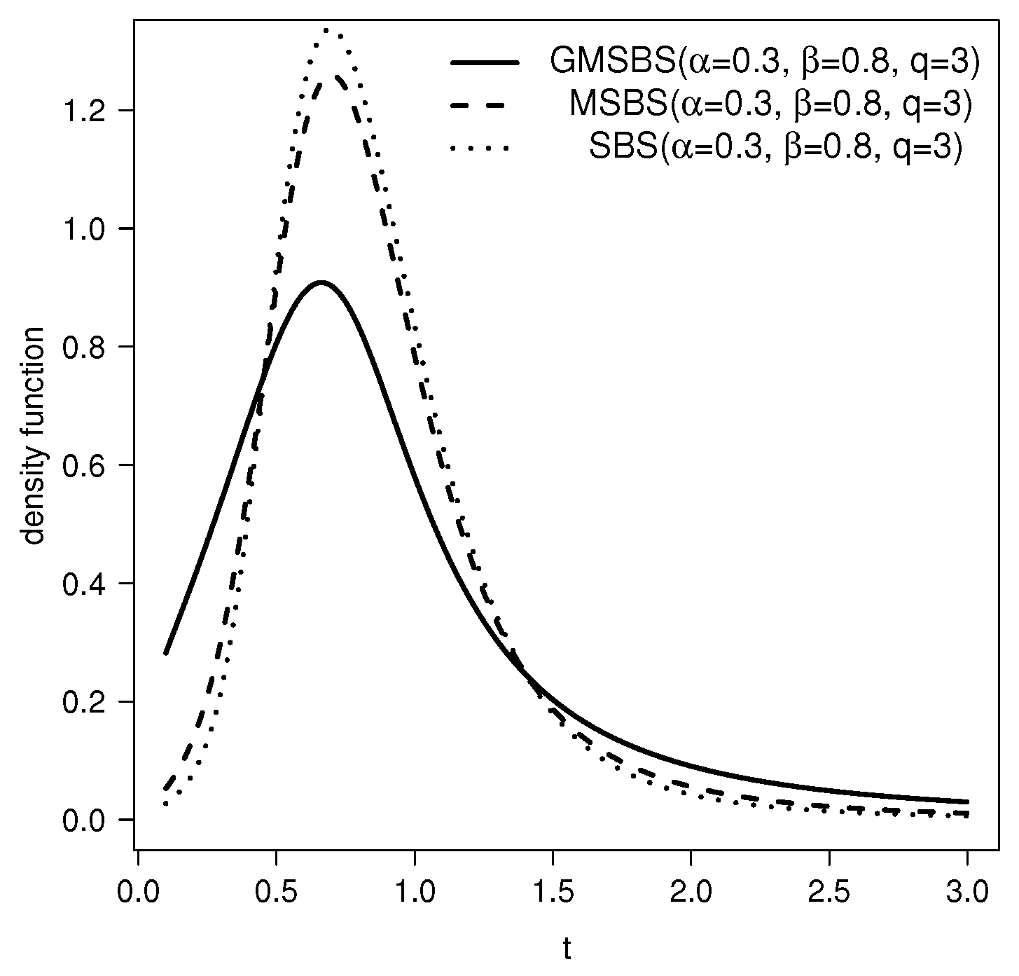
2. GMSBS Distributions
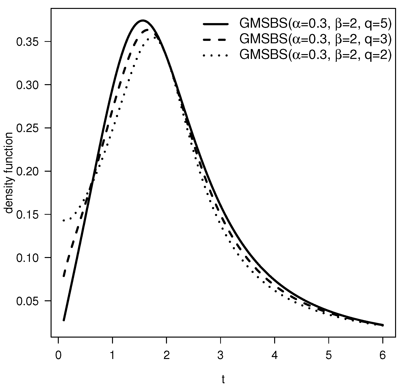
2.1. Probability Density Function
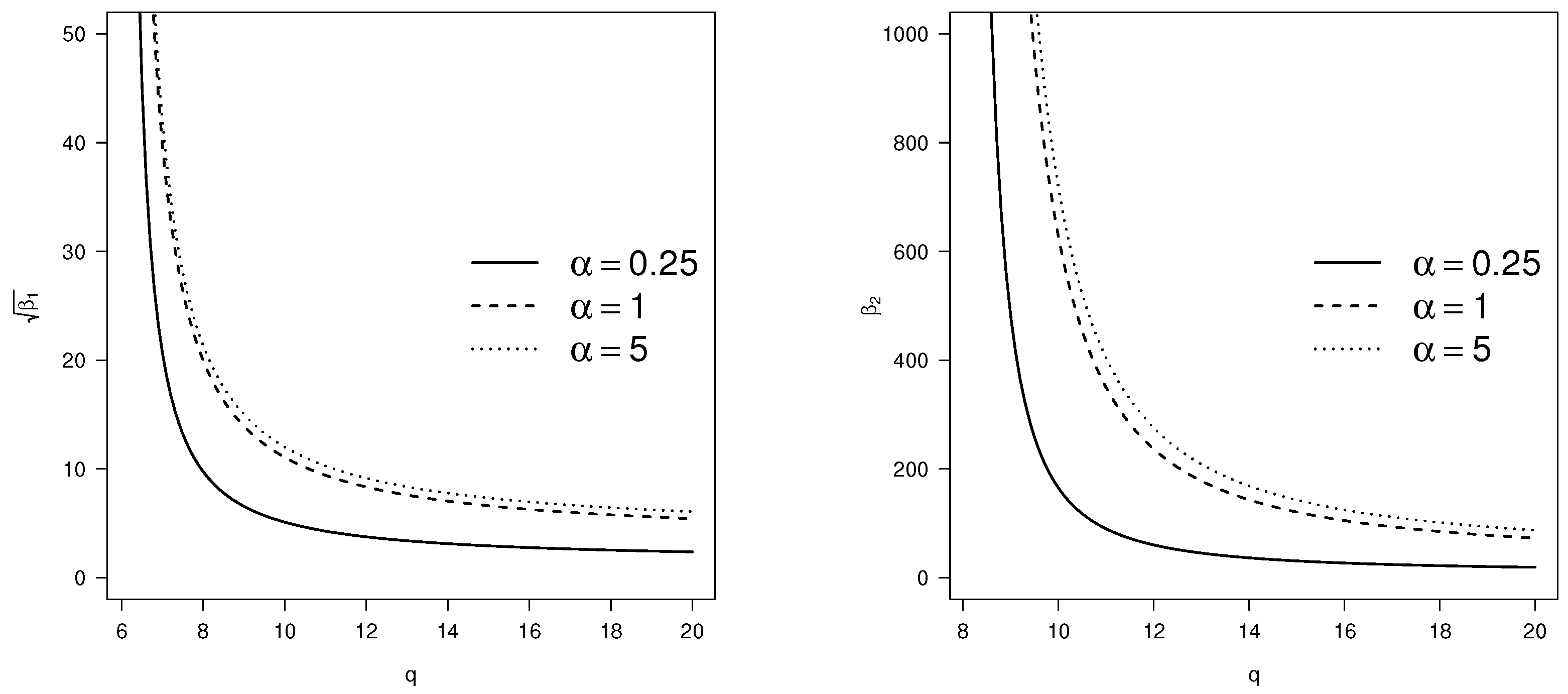
2.2. Properties
- 1.
- Let be the pth quantile of T, .where denotes the pth quantile ofIn particular, the median of T is β, .
- 2.
- , .
- 3.
- .
2.3. Moments
3. Estimation
3.1. Modified Moment Estimation
3.2. Maximum Likelihood Estimation
3.3. ML Estimation Using EM-Algorithm
4. Simulation
- Simulate
- Simulate with .
- Compute Then, ,
- Compute , , . for
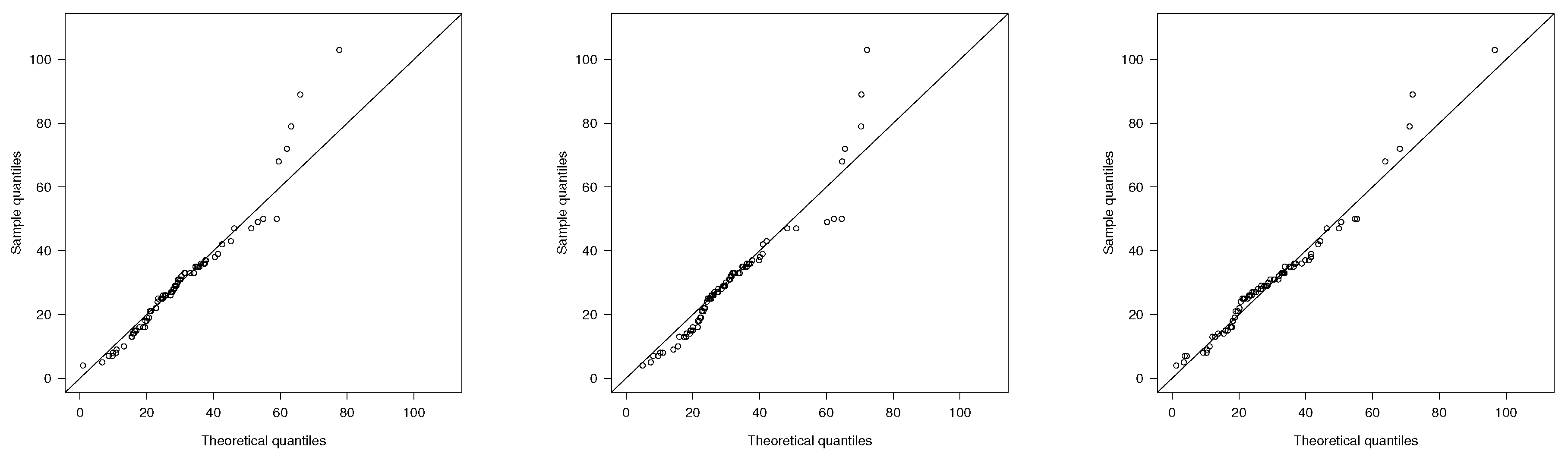
5. Applications
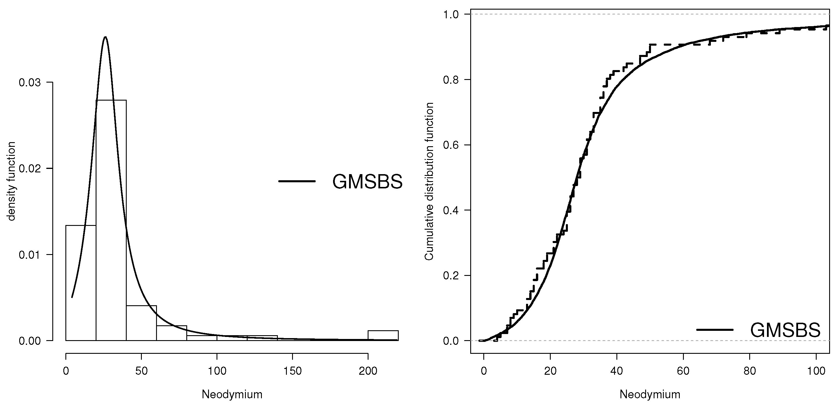
5.1. Neodymium Dataset
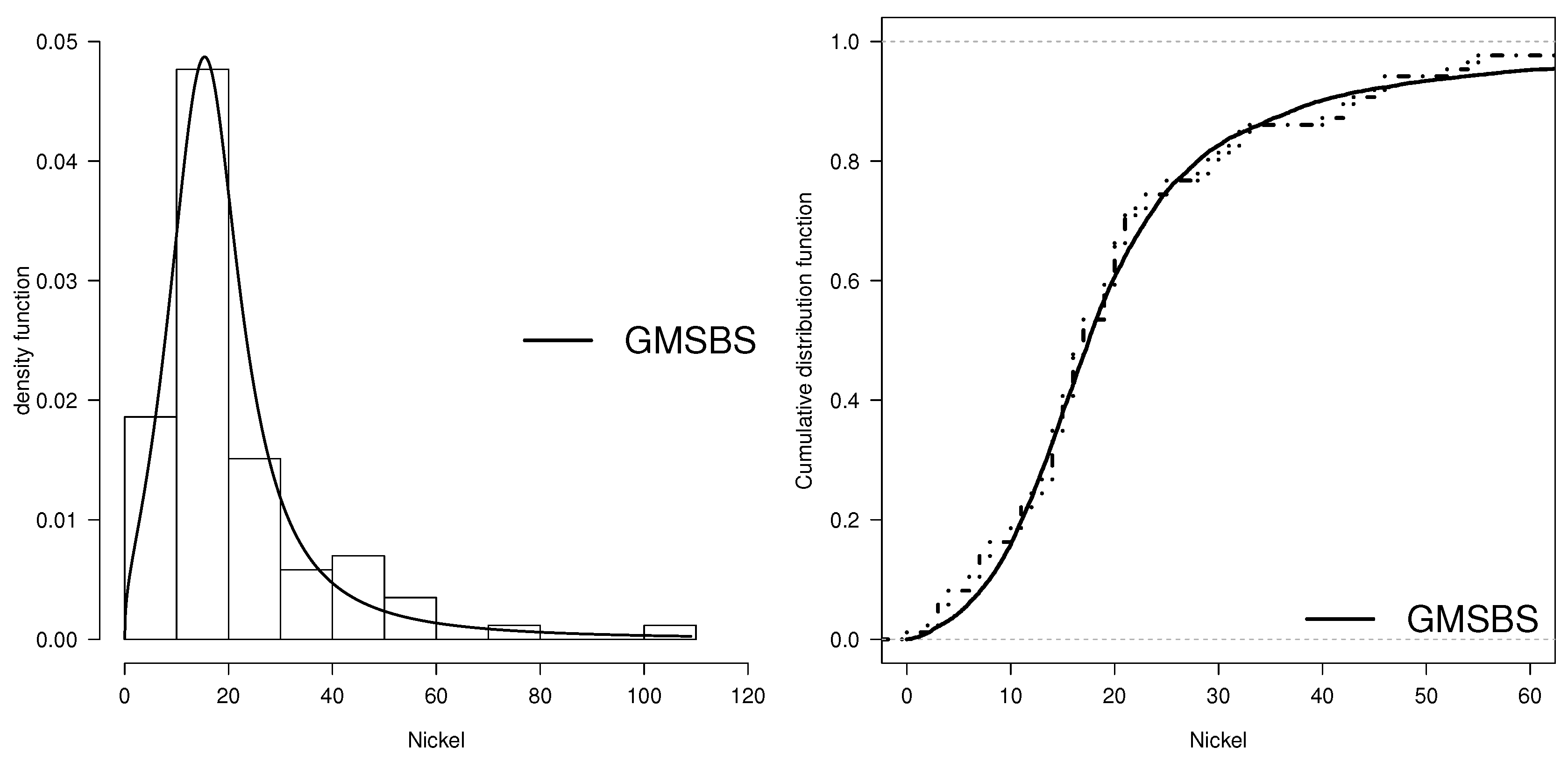
5.2. Nickel Dataset
Author Contributions
Funding
Acknowledgments
Conflicts of Interest
Appendix A. Some Proofs of Results Given in Section 2
Appendix B. Likelihood Equations
References
- Birnbaum, Z.W.; Saunders, S.C. A New Family of Life Distributions. J. Appl. Probab. 1969, 6, 319–327. [Google Scholar] [CrossRef]
- Birnbaum, Z.W.; Saunders, S.C. Estimation for a family of life distributions with applications to fatigue. J. Appl. Probab. 1969a, 6, 328–347. [Google Scholar] [CrossRef]
- Moors, J.J.A. A quantile alternative for kurtosis. J. R. Stat. Soc. Ser. D 1988, 37, 25–32. [Google Scholar] [CrossRef]
- Johnson, N.L.; Kotz, S.; Balakrishnan, N. Continuous Univariate Distributions, 2nd ed.; Wiley: New York, NY, USA, 1995; Volume 1. [Google Scholar]
- Leiva, V. The Birnbaum–Saunders Distribution; Academic Press: New York, NY, US, 2016. [Google Scholar]
- Gómez, H.W.; Olivares-Pacheco, J.F.; Bolfarine, H. An extension of the generalized Birnbaum–Saunders distribution. Stat. Probab. Lett. 2009, 79, 331–338. [Google Scholar] [CrossRef]
- Reyes, J.; Gómez, H.W.; Bolfarine, H. Modified slash distribution. Stat. J. Theor. App. Stat. 2013, 47, 929–941. [Google Scholar] [CrossRef]
- Rogers, W.H.; Tukey, J.W. Understanding some long-tailed symmetrical distributions. Stat. Neerl. 1972, 26, 211–226. [Google Scholar] [CrossRef]
- Reyes, J.; Barranco-Chamorro, I.; Gómez, H.W. Generalized modified slash distribution. 2018. Submitted. [Google Scholar]
- Abramowitz, M.; Stegun, I.A. Handbook of Mathematical Functions, 10th ed.; Handbook of Mathematical Functions: Dover, NY, USA, 1972. [Google Scholar]
- Reyes, J.; Vilca, F.; Gallardo, D.I.; Gómez, H.W. Modified slash Birnbaum–Saunders distribution. Hacettepe J. Math. Stat. Ser. B 2017, 46, 969–984. [Google Scholar] [CrossRef]
- Ng, H.; Kundu, D.; Balakrishnan, N. Modified moment estimation for the two-parameter Birnbaum–Saunders distribution. Comput. Stat. Data Anal. 2003, 43, 283–298. [Google Scholar] [CrossRef]
- Dempster, A.P.; Rubin, D.B.; Laird, N.M. Maximum likelihood from incomplete data via the EM algorithm (with discussion). J. R. Stat. Soc. B 1977, 39, 1–38. [Google Scholar]
- Lee, S.Y.; Xu, L. Influence analyses of nonlinear mixed-effects model. Comput. Stat. Data Anal. 2004, 45, 321–341. [Google Scholar] [CrossRef]
- Lin, X.S.; Liu, X. Markow aging process and phase-type law of mortality. N. Am. Actuar. J. 2007, 11, 92–109. [Google Scholar] [CrossRef]
- Akaike, H. A new look at the statistical model identification. IEEE Trans. Autom. Control 1974, 19, 716–723. [Google Scholar] [CrossRef]
- Rohatgi, V.K.; Ehsanes Saleh, A.K.M.D. An Introduction to Probability and Statistics, 3rd ed.; John Wiley and Sons: New York, NY, USA, 2001. [Google Scholar]


| True Value | ||||||||||||
|---|---|---|---|---|---|---|---|---|---|---|---|---|
| bias | s.e. | bias | s.e. | bias | s.e. | |||||||
| 1 | 2 | 2 | 0.0578 | 0.2267 | 0.2327 | 0.0455 | 0.1596 | 0.1588 | 0.0373 | 0.1110 | 0.1113 | |
| 0.1191 | 0.6707 | 0.7412 | 0.0702 | 0.4794 | 0.4953 | 0.0367 | 0.3273 | 0.3352 | ||||
| 1.0222 | 1.8522 | 3.5878 | 0.3839 | 0.7437 | 1.2601 | 0.1959 | 0.4183 | 0.4789 | ||||
| 2 | 0.1373 | 0.4633 | 0.4914 | 0.1012 | 0.3235 | 0.3282 | 0.0753 | 0.2290 | 0.2279 | |||
| 0.1871 | 0.9125 | 1.0495 | 0.0635 | 0.6299 | 0.6729 | 0.0489 | 0.4542 | 0.4677 | ||||
| 1.3715 | 2.2452 | 5.0045 | 0.3781 | 0.7066 | 0.9840 | 0.1812 | 0.4254 | 0.4560 | ||||
| 3 | 0.2858 | 0.7062 | 0.7504 | 0.1563 | 0.4872 | 0.4798 | 0.1264 | 0.3398 | 0.3385 | |||
| 0.2776 | 0.9688 | 1.1139 | 0.1234 | 0.6537 | 0.7049 | 0.0535 | 0.4630 | 0.4451 | ||||
| 1.2999 | 2.0412 | 4.3190 | 0.3930 | 0.7107 | 0.9874 | 0.1928 | 0.4161 | 0.4836 | ||||
| 1 | 1 | 1 | 0.1946 | 0.3061 | 0.6894 | 0.1402 | 0.2041 | 0.2457 | 0.1535 | 0.1373 | 0.3721 | |
| 0.2621 | 0.4270 | 4.8105 | 0.0401 | 0.2711 | 0.2847 | 0.0333 | 0.1870 | 0.1996 | ||||
| 0.3416 | 0.4464 | 0.6948 | 0.2206 | 0.2528 | 0.3243 | 0.1723 | 0.1647 | 0.2305 | ||||
| 2 | 0.1741 | 0.3155 | 0.3550 | 0.1443 | 0.2088 | 0.2595 | 0.1461 | 0.1326 | 0.3455 | |||
| 0.1844 | 0.8233 | 0.9462 | 0.0805 | 0.5533 | 0.5930 | 0.0465 | 0.3566 | 0.3866 | ||||
| 0.3206 | 0.4777 | 0.8124 | 0.2104 | 0.2537 | 0.3223 | 0.1745 | 0.1609 | 0.2323 | ||||
| 3 | 0.1689 | 0.3042 | 0.4005 | 0.1405 | 0.2041 | 0.3346 | 0.1351 | 0.1348 | 0.2716 | |||
| 0.3346 | 1.2332 | 2.3262 | 0.1246 | 0.7904 | 0.8285 | 0.0445 | 0.5271 | 0.5435 | ||||
| 0.3351 | 0.4584 | 0.6384 | 0.2132 | 0.2594 | 0.3229 | 0.1701 | 0.1608 | 0.2274 | ||||
| 0.5 | 1 | 1 | 0.0734 | 0.1447 | 0.1658 | 0.0712 | 0.0987 | 0.1625 | 0.0667 | 0.0659 | 0.1430 | |
| 0.0314 | 0.1952 | 0.2170 | 0.0091 | 0.1306 | 0.1365 | 0.0064 | 0.0889 | 0.1240 | ||||
| 0.2724 | 0.4067 | 0.5825 | 0.2005 | 0.2432 | 0.3146 | 0.1656 | 0.1588 | 0.2270 | ||||
| 2 | 0.0196 | 0.1174 | 0.1117 | 0.0173 | 0.0783 | 0.0732 | 0.0183 | 0.0566 | 0.0570 | |||
| 0.0193 | 0.1848 | 0.1798 | 0.0080 | 0.1237 | 0.1215 | 0.0041 | 0.0879 | 0.0836 | ||||
| 0.9310 | 1.7205 | 4.1727 | 0.2917 | 0.6519 | 0.7662 | 0.1691 | 0.4138 | 0.4612 | ||||
| 3 | 0.0138 | 0.0993 | 0.0995 | 0.0148 | 0.0695 | 0.0660 | 0.0110 | 0.0488 | 0.0482 | |||
| 0.0118 | 0.1663 | 0.1742 | 0.0133 | 0.1207 | 0.1182 | 0.0009 | 0.0829 | 0.0832 | ||||
| 2.4498 | 4.3431 | 7.8277 | 0.7645 | 1.4680 | 3.0066 | 0.2994 | 0.7723 | 0.9407 | ||||
| n | ||||
|---|---|---|---|---|
| 86 | 35.02 | 35.2307 | 3.648 | 18.216 |
| Parameter | SBS | MSBS | GMSBS |
|---|---|---|---|
| 0.289 (0.064) | 0.290 (0.105) | 0.2087 (0.0366) | |
| 27.247 (1.592) | 27.683 (5.983) | 28.1102 (1.4994) | |
| q | 1.578 (0.426) | 2.009 (0.570) | 2.5661 (0.9489) |
| AIC | 743.9906 | 741.3566 | 739.9394 |
| n | ||||
|---|---|---|---|---|
| 85 | 21.59 | 16.5732 | 2.3922 | 11.325 |
| Parameter | SBS | MSBS | GMSBS |
|---|---|---|---|
| 0.3877 (0.0918) | 0.3266 (0.0852) | 0.2490 (0.0330) | |
| 17.7982 (1.2464) | 17.6017 (1.1027) | 17.4961 (1.0622) | |
| q | 2.0118 (0.6967) | 2.0932 (0.6284) | 3.1927 (1.2341) |
| AIC | 670.742 | 668.251 | 666.571 |
© 2018 by the authors. Licensee MDPI, Basel, Switzerland. This article is an open access article distributed under the terms and conditions of the Creative Commons Attribution (CC BY) license (http://creativecommons.org/licenses/by/4.0/).
Share and Cite
Reyes, J.; Barranco-Chamorro, I.; Gallardo, D.I.; Gómez, H.W. Generalized Modified Slash Birnbaum–Saunders Distribution. Symmetry 2018, 10, 724. https://doi.org/10.3390/sym10120724
Reyes J, Barranco-Chamorro I, Gallardo DI, Gómez HW. Generalized Modified Slash Birnbaum–Saunders Distribution. Symmetry. 2018; 10(12):724. https://doi.org/10.3390/sym10120724
Chicago/Turabian StyleReyes, Jimmy, Inmaculada Barranco-Chamorro, Diego I. Gallardo, and Héctor W. Gómez. 2018. "Generalized Modified Slash Birnbaum–Saunders Distribution" Symmetry 10, no. 12: 724. https://doi.org/10.3390/sym10120724
APA StyleReyes, J., Barranco-Chamorro, I., Gallardo, D. I., & Gómez, H. W. (2018). Generalized Modified Slash Birnbaum–Saunders Distribution. Symmetry, 10(12), 724. https://doi.org/10.3390/sym10120724