Numerical Investigation of Heat Conduction with Multiple Moving Heat Sources

Abstract

This paper is concerned about the efficiently numerical simulation of heat conduction problems with multiple heat sources that are allowed to move with different speeds. Based on the dynamical domain decomposition upon the trajectories of moving sources, which are solved by a predictor–corrector algorithm, a non-overlapping domain-decomposed moving mesh method is developed. Such a method can not only generate the adaptive mesh efficiently by parallel computing, but also greatly simplify the discretization of the underlying equations without loss of accuracy. Numerical examples for various motions of sources are presented to illustrate the accuracy, the convergence rate and the efficiency of the proposed method. The dependence of the solution on the moving sources such as the types of motion and the distance between sources is numerically investigated. A blow-up phenomenon that occurs at multiple locations simultaneously can also be well observed for the case of symmetrically moving sources.

1. Introduction

The heat conduction transfer of problems with moving heat sources has attracted a great deal of interest by engineers in the past few decades. Typical applications include contact surfaces such as free-boundary solidification [1], and many metallurgical processes such as laser cutting and welding [2,3,4,5]. Mathematically, this problem can be well modeled by the heat conduction equation with singular source terms, which utilize a time-dependent delta function to describe each highly localized and moving heat source (see [1,3,6,7] and references therein). It is well known nowadays that the solution of such a model equation is continuous and piecewise smooth with a jump for derivative of the solution when crossing each heat source [8]. It has also been proved theoretically that blow-up may occur at some location in a finite time, if one of the source strengths can not be neglected and the corresponding source is traveling with a relatively low speed [7]. Due to these singularities, numerical simulation to investigate the solution phenomenon, such as the prediction of the blow-up time, accurately and efficiently still remains big challenges.

When the singularity behaves in a time-dependent localized region, adaptive mesh methods are more popular than the numerical methods using a fixed mesh, which always leads to a huge computational cost to preserve accuracy, as the solution evolves singularity. Among the adaptive mesh methods, this paper is mainly concerned about the moving mesh method, which is easy to use and has been successfully applied to investigate the blow-up phenomenon [9,10] and other time-dependent localized singularities [11,12,13,14]. The moving mesh, which continuously adjusts the locations of mesh points to resolve the solution as well as possible with a fixed total number of mesh points, can be generated adaptively by the moving mesh partial differential equations (MMPDEs) derived from the equidistribution principle [15,16]. Based on the Schwarz domain decomposition method, one of the overlapping domain decomposition methods, the parallel generation of moving mesh has been studied in recent years [17,18,19].

For problems with moving heat sources, a second-order moving mesh method has been developed for one source case in [20], where the source trajectory is given explicitly and the delta function is approximated in the final discretization by appropriate information of jumps. Some modifications, to simplify the discretization without loss of accuracy, have been proposed and extended to multiple sources case in [21,22]. However, all of these moving mesh methods were only presented for the one source case or the multiple sources case that all sources are moving with the same speed. Nevertheless, it becomes too complicated for [20,21] and even impossible for [22] to extend the corresponding method to the situation that the sources are moving with different speeds. Moreover, it is worth mentioning that these methods are usually failed to capture the blow-up phenomenon occurring at multiple locations simultaneously. Even worse, these methods can not be smoothly generalized to multi-dimensional situations, since it is difficult to define appropriate jumps of solution caused by the delta function as in a one-dimensional case.

Motivated by the above observation, this paper focuses on the development of the moving mesh method for problems with multiple moving heat sources, whose motions are controlled by different ordinary differential equations. The main idea and novelty is to decompose the domain dynamically according to the locations of moving heat sources, such that there exists a fixed mesh point moving exactly along the trajectory of each source, which is solved by a predictor–corrector algorithm. In each time-dependent subdomain, an MMPDE is applied to find the local equidistributed mesh. The model equation is then solved on the adaptive mesh assembling from local mesh on each subdomain. There are many advantages of the present method in comparison to the methods proposed in [20,21,22]:

• Firstly, the adaptive mesh is optimal in the sense of equidistribution on each subdomain, and can be generated very efficiently, since the local equidistributed mesh on each subdomain can be obtained in parallel.
• Secondly, it is found that the jump $\left[\dot{u}\right]$ always vanishes on the specially designed adaptive mesh. Consequently, the discretization of the underlying model equation is further simplified while maintaining a second-order convergence rate in space. Moreover, the derived discretization is reinterpreted from a novel perspective, which shows some inspiration to extend the proposed method to a multi-dimensional case.
• Thirdly, with the help of exact tracing of each heat source by a fixed mesh point, the blow-up phenomenon that occurs at multiple locations simultaneously has been successfully observed by the present numerical experiment of symmetrically moving sources.
• Finally, various numerical experiments are carried out to investigate the solution behavior in terms of the motions of heat sources, such as the types of motion and the distance between the sources. The blow-up phenomena in terms of the distance of two moving sources are numerically discussed. It is found as expected that, if the sources are moving with high speeds, there may exist a critical distance, such that blow-up must occur if the distance of the sources is less than the critical distance, while blow-up is avoided when the distance is larger than this critical distance.

The rest of this paper is organized as follows. The model equation for multiple moving heat sources problem is briefly introduced in Section 2. The detailed numerical method is described in Section 3. Numerical examples are exhibited in Section 4 to validate the accuracy and the efficiency of the present method, and to investigate the solution behavior for various motions of heat sources. Some conclusions are given in the last section.

2. Model Equation

The temperature distribution in a reactive-diffusive material with multiple moving heat sources can be well described by the following equation [7,20]:

$$\begin{array}{c}{u}_t-u_{xx}=\sum _{i=0}^{q-1}{F}_i\left(u(x,t)\right)\delta (x-{\alpha }_i\left(t\right)),-\infty <x<\infty ,t>0,\hfill \end{array}$$

(1)

with the initial and boundary conditions

$$\begin{array}{c}u(x,0)=u_0\left(x\right),-\infty <x<\infty ,\hfill \end{array}$$

(2)

$$\begin{array}{c}u(x,t)\to 0\mathrm{as}\left|x\right|\to \infty ,t>0,\hfill \end{array}$$

(3)

where $u(x,t)$ is the temperature, with $u_t$ and $u_{xx}$ representing its first order partial derivative with respect to t and its second order partial derivative with respect to x, respectively. The function $u_0\left(x\right)$ is continuous with $u_0\left(x\right)\to 0$ as $\left|x\right|\to \infty$, and q is the number of heat sources. The ith heat source, which is modeled by the Dirac delta function $\delta (x-{\alpha }_i\left(t\right))$ with the source function $F_i\left(u\right)$, is moving along the curve ${\alpha }_i\left(t\right)$, and its velocity is determined by

$$\begin{array}{c}\hfill \frac{\mathrm{d}{\alpha }_i\left(t\right)}{\mathrm{d}t}={\psi }_i(t,{\alpha }_i\left(t\right),u({\alpha }_i\left(t\right),t)),\end{array}$$

(4)

where ${\psi }_i$ is a given function that may depend on the local temperature $u({\alpha }_i\left(t\right),t)$. Currently, the author focuses on the case that all sources do not intersect with each other during the time in consideration. Additionally, the source function $F_i\left(u\right)$ is usually a nonlinear function of u, and it has been proved [6,7] that blow-up may occur at some location in a finite time T, i.e., $\underset{t\to T}{lim}max\left\{u(x,t)\right\}\to +\infty$, if one of the source functions, namely $F_{i_0}\left(u\right)$, satisfies

$$F_{i_0}\left(u\right)>0,F_{i_0}^{\prime }\left(u\right)>0,F_{i_0}^{″}\left(u\right)>0,\mathrm{for}u>0,$$

and the corresponding source is moving with a sufficiently low speed, that is, $|{\alpha }_{i_0}^{\prime }\left(t\right)|\le \kappa$, where $\kappa$ is an appropriate constant.

3. Numerical Method

This section is going to develop a numerical method to solve the model Problems (1)–(4) accurately and efficiently on a bounded domain $[x_l\left(t\right),x_r\left(t\right)]$ that contains all heat sources. I will first introduce an adaptive mesh generated by the domain-decomposed moving mesh method and then give the detailed discretization of the underlying model equations on this special mesh. The final algorithm will then be presented. Without loss of generality, let us assume that $x_l\left(t\right)<{\alpha }_0\left(t\right)<{\alpha }_1\left(t\right)<\cdots <{\alpha }_{q-1}\left(t\right)<x_r\left(t\right)$.

3.1. Domain-Decomposed Adaptive Mesh Generation

Upon the locations of the moving heat sources, the physical domain $[x_l\left(t\right),x_r\left(t\right)]$ is dynamically divided into $q+1$ subdomains $[{\alpha }_{i-1}\left(t\right),{\alpha }_i\left(t\right)]$, $i=0,1,\dots ,q$, where ${\alpha }_{-1}\left(t\right)=x_l\left(t\right)$ and ${\alpha }_q\left(t\right)=x_r\left(t\right)$. Suppose that there exists a one-to-one coordinate transformation $x=x(\xi ,t)$ between the physical domain $[x_l\left(t\right),x_r\left(t\right)]$ and the computational domain $[0,1]$, such that $x(0,t)=x_l\left(t\right)$, and $x(1,t)=x_r\left(t\right)$. For a given uniform mesh, ${\xi }_j=\frac{j}{N}$, $j=0,1,\dots ,N$, on the computational domain, we have the corresponding mesh $\mathcal{G}=\left\{x_j\left(t\right)\right\}$ on the physical domain, where $x_j\left(t\right)=x({\xi }_j,t)$, and

$$x_l\left(t\right)=x_0\left(t\right)<x_1\left(t\right)<\cdots <x_N\left(t\right)=x_r\left(t\right).$$

Let $N=(q+1)K$ and further assume that the $(i+1)K$th mesh point captures the ith source exactly, i.e., $x_{(i+1)K}\left(t\right)\equiv {\alpha }_i\left(t\right)$. It is easy to show that each physical subdomain $[{\alpha }_{i-1}\left(t\right),{\alpha }_i\left(t\right)]$ is discretized by $K+1$ mesh points, namely, $x_{iK}\left(t\right),x_{iK+1}\left(t\right),\dots ,x_{(i+1)K}\left(t\right)$. However, I remind readers that it is not necessary to discretize each subdomain with the same number of mesh points.

In each physical subdomain $[{\alpha }_{i-1}\left(t\right),{\alpha }_i\left(t\right)]$, the moving mesh method is used to adaptively adjust the mesh such that the appropriately defined monitor function $M=M(t,x,u)$ is equidistributed. The monitor function plays a key role in the moving mesh method [16], and will be given in Section 4 for our numerical experiments. Among the popular moving mesh partial differential equations (MMPDEs) proposed in [15] to equidistribute the monitor function, the so-called MMPDE6, which reads

$$\frac{{\partial }^2\dot{x}}{\partial {\xi }^2}=-\frac{1}{\tau }\frac{\partial }{\partial \xi }\left(M\frac{\partial x}{\partial \xi }\right),$$

(5)

is employed as an example in this paper. Here, $\dot{x}$ is the first order partial derivative of x with respect to t, and $\tau$ is a user-defined positive number for adjusting the time scale of the mesh equation. With boundary conditions

$$x_{iK}\left(t\right)={\alpha }_{i-1}\left(t\right),x_{(i+1)K}\left(t\right)={\alpha }_i\left(t\right),$$

(6)

the MMPDE6 (5) can be solved by the following finite difference discretization

$$\begin{array}{c}\frac{\left(x_{j+1}^{n+1}-2x_j^{n+1}+x_{j-1}^{n+1}\right)-\left(x_{j+1}^n-2x_j^n+x_{j-1}^n\right)}{\Delta t_n}\\ =-\frac{1}{\tau }\left(M_{j+\frac{1}{2}}^n\left(x_{j+1}^{n+1}-x_j^{n+1}\right)-M_{j-\frac{1}{2}}^n\left(x_j^{n+1}-x_{j-1}^{n+1}\right)\right),\end{array}$$

(7)

for $j=iK+1,iK+2,\dots ,(i+1)K-1$. Here, $\Delta t_n=t_{n+1}-t_n$ is the time step length, $M_{j+\frac{1}{2}}^n=\left(M_{j+1}^n+M_j^n\right)/2$ is the average of discrete monitor function on the jth and $(j+1)$th mesh points, and $x_j^n$ is the numerical approximation of $x({\xi }_j,t_n)$. When Equation (7) together with boundary Conditions (6) have been solved on all subdomains, we then get the new mesh ${\mathcal{G}}^{n+1}=\left\{x_j^{n+1}\right\}$ for the whole domain $[x_l\left(t_{n+1}\right),x_r\left(t_{n+1}\right)]$ (see Figure 1 for the sketch of the above mesh generation). Again, it is not necessary to utilize the same monitor function and the same MMPDE in each subdomain. Thus, the present mesh generation strategy is very flexible. It is also pointed out that such an adaptive mesh can be obtained very efficiently by parallel computing based on domain decomposition methods [23]. Moreover, it is optimal in the sense of equidistribution of the monitor function on each subdomain. Further advantages of such a mesh can be obtained in the discretization of the model Equation (1), which will be given in the next subsection.

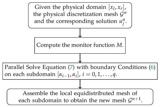
Figure 1. The sketch of domain-decomposed moving mesh generation.

3.2. Discretization on the Moving Mesh

Now, it is ready to introduce the discretization of the underlying Equations (1) and (4) on the adaptive moving mesh generated in the previous subsection.

For an arbitrary function $f=f(x,t)=f\left(x\right(\xi ,t),t)$, we have

$$\dot{f}:=\frac{\partial f}{\partial t}(x(\xi ,t),t){|}_{\xi \mathrm{fixed}}=f_t+f_x\dot{x},$$

where $f_t$ and $f_x$ are the first order derivatives of f with respect to t and x, respectively. Consequently, the original Equation (1) can be rewritten into

$$\begin{array}{c}\hfill \dot{u}-u_x\dot{x}-u_{xx}=\sum _{i=0}^{q-1}{F}_i\left(u(x,t)\right)\delta (x-{\alpha }_i\left(t\right)).\end{array}$$

(8)

When $x\ne {\alpha }_i\left(t\right)$, it is obvious that the above equation reduces to the following equation:

$$\dot{u}-u_x\dot{x}-u_{xx}=0.$$

(9)

Therefore, one may derive the discretization of Equation (8) based on the standard finite difference discretization of Equation (9), with modifications containing appropriate information of jumps when the mesh line of stencil mesh points intersects with one of the trajectories of heat sources. The jump of a given function $\phi$ along the smooth curve $\left(\theta \right(\lambda ),\vartheta (\lambda \left)\right)$ at the crossing point $(\overline{x},\overline{t})$ is defined by [20]

$${\left[\phi \right]}_{(\overline{x},\overline{t})}:=\underset{\epsilon \to 0^{+}}{lim}\left(\phi \left(\theta (\overline{\lambda }+\epsilon ),\vartheta (\overline{\lambda }+\epsilon )\right)-\phi \left(\theta (\overline{\lambda }-\epsilon ),\vartheta (\overline{\lambda }-\epsilon )\right)\right),$$

where $(\theta \left(\overline{\lambda }\right),\vartheta \left(\overline{\lambda }\right))=(\overline{x},\overline{t})$. Then, from Equation (8), we have

$${\left[u\right]}_{({\alpha }_i\left(t\right),t)}=0,{\left[u_x\right]}_{({\alpha }_i\left(t\right),t)}=-F_i\left(u({\alpha }_i\left(t\right),t)\right),i=0,1,\cdots ,q-1.$$

(10)

Physically, the value $u({\alpha }_i\left(t\right),t)$ changes smoothly as time evolves [20]. It follows that the jump of the directional derivative of $u(x,t)$ along the vector $({\alpha }_i^{\prime }\left(t\right),1)$ is zero. By noting that, for the designed adaptive moving mesh, there is a mesh point that moves exactly along the trajectory of each heat source, we then obtain

$${\left[\dot{u}\right]}_{({\alpha }_i\left(t\right),t)}={[u_t+u_x\dot{x}]}_{({\alpha }_i\left(t\right),t)}={\left[u_t\right]}_{({\alpha }_i\left(t\right),t)}+\dot{x}{\left[u_x\right]}_{({\alpha }_i\left(t\right),t)}={\left[u_t\right]}_{({\alpha }_i\left(t\right),t)}+{\alpha }_i^{\prime }\left(t\right){\left[u_x\right]}_{({\alpha }_i\left(t\right),t)}=0,$$

(11)

$i=0,1,\dots ,q-1$. Additionally, we can deduce that

$$\begin{array}{c}{\left[u_{xx}\right]}_{({\alpha }_i\left(t\right),t)}={\left[\dot{u}\right]}_{({\alpha }_i\left(t\right),t)}-\dot{x}{\left[u_x\right]}_{({\alpha }_i\left(t\right),t)}=-{\alpha }_i^{\prime }\left(t\right){\left[u_x\right]}_{({\alpha }_i\left(t\right),t)}={\psi }_i(t,{\alpha }_i\left(t\right),u({\alpha }_i\left(t\right),t))F_i\left(u({\alpha }_i\left(t\right),t)\right),\end{array}$$

(12)

$i=0,1,\dots ,q-1$.

With the above information of jumps, the discretization of Equation (8), which has second-order convergence rate in space, is finally divided into two categories according to the position of the mesh point. Specifically, if the mesh point does not locate at the heat source, that is, $j=0,1,\dots ,N$, but $j\ne (i+1)K$, $i=0,1,\dots ,q-1$, we have the standard central difference discretization

$$\frac{u_j^{n+1}-u_j^n}{\Delta t_n}-\frac{u_{j+1}^{n+1}-u_{j-1}^{n+1}}{h_{j+1}^{n+1}+h_j^{n+1}}\left(\frac{x_j^{n+1}-x_j^n}{\Delta t_n}\right)-\frac{2}{h_{j+1}^{n+1}+h_j^{n+1}}\left(\frac{u_{j+1}^{n+1}-u_j^{n+1}}{h_{j+1}^{n+1}}-\frac{u_j^{n+1}-u_{j-1}^{n+1}}{h_j^{n+1}}\right)=0,$$

(13)

where $x_j^n=x({\xi }_j,t_n)$, $h_j^n=x_j^n-x_{j-1}^n$ and $u_j^n$ is the numerical approximation of the solution $u(x_j^n,t_n)$. If the mesh point does exactly locate at the ith heat source, $i=0,\cdots ,q-1$, we have to incorporate the jump information into the discretization, which gives

$$\begin{array}{cc}\hfill \frac{u_j^{n+1}-u_j^n}{\Delta t_n}-\frac{u_{j+1}^{n+1}-u_{j-1}^{n+1}}{h_{j+1}^{n+1}+h_j^{n+1}}{\psi }_i^{n+1}& -\frac{2}{h_{j+1}^{n+1}+h_j^{n+1}}\left(\frac{u_{j+1}^{n+1}-u_j^{n+1}}{h_{j+1}^{n+1}}-\frac{u_j^{n+1}-u_{j-1}^{n+1}}{h_j^{n+1}}\right)\hfill \\ & -\frac{2}{h_{j+1}^{n+1}+h_j^{n+1}}{F}_i\left(u_j^{n+1}\right)=0,\hfill \end{array}$$

(14)

where $j=(i+1)K$ and ${\psi }_i^{n+1}$ is the numerical approximation of ${\psi }_i(t_{n+1},{\alpha }_i\left(t_{n+1}\right),u_j^{n+1})$. For the detailed derivation of the above discretization, I refer the readers to [20]. However, it is worth pointing out that, in [20], five cases must be considered for the discretization of Equation (8), even when there is only one heat source.

Remark 1.

In the famous immerse boundary method [1,24], the delta function is first replaced by a suitable discrete approximation, which is usually the “hat function” with a fixed width support. Then, the resulting equation is discretized using standard numerical methods on the uniform grid. If now we approximate each delta function $\delta (x-{\alpha }_i\left(t\right))$ in Equation (8) by the hat function defined as

$$\begin{array}{c}\hfill d_{h,i}(x,t)=\left\{\begin{array}{cc}{\displaystyle \frac{2}{h_{j+1}\left(t\right)+h_j\left(t\right)}}·{\displaystyle \frac{x-x_{j-1}\left(t\right)}{h_j\left(t\right)}},\hfill & x_{j-1}\left(t\right)\le x\le x_j\left(t\right),\hfill \\ {\displaystyle \frac{2}{h_{j+1}\left(t\right)+h_j\left(t\right)}}·{\displaystyle \frac{x-x_{j+1}\left(t\right)}{h_{j+1}\left(t\right)}},\hfill & x_j\left(t\right)\le x\le x_{j+1}\left(t\right),\hfill \\ 0,\hfill & \mathit{otherwise},\hfill \end{array}\right.\end{array}$$

where $h_j\left(t\right)=x_j\left(t\right)-x_{j-1}\left(t\right)$ and $j=(i+1)K$, then applying the standard finite difference method for the resulting equation

$$\begin{array}{c}\hfill \dot{u}-u_x\dot{x}-u_{xx}=\sum _{i=0}^{q-1}{F}_i\left(u(x,t)\right)d_{h,i}(x,t)\end{array}$$

on the designed adaptive moving mesh $\mathcal{G}=\left\{x_j\left(t\right)\right\}$ would also give the same discretization as Equations (13) and (14).

From the above point of view, first replacing the delta function by a mesh-dependent discrete approximation and then discretizing the resulting equation by standard numerical methods, one could obtain higher-order discretization both in space and time without much effort. It also shows some inspiration to extend the present method to multi-dimensional situation since the definition of jump is completely avoided, and this will be further studied in our future work.

Apparently, we need to know the source position ${\alpha }_i\left(t_{n+1}\right)$ before solving the system of Equations (13) and (14). If ${\psi }_i$ in Equation (4) is independent from u, one may only employ the following Crank–Nicolson scheme

$$\begin{array}{c}\hfill {\alpha }_i^{n+1}={\alpha }_i^n+\frac{\Delta t_n}{2}({\psi }_i^{n+1}+{\psi }_i^n),i=0,1,\dots ,q-1,\end{array}$$

(15)

to update the source position ${\alpha }_i^{n+1}\approx {\alpha }_i\left(t_{n+1}\right)$ as in [22,25]. Otherwise, a predictor–corrector iteration will be employed to update the source position ${\alpha }_i^{n+1}$, the mesh points $x_j^{n+1}$ and the solution $u_j^{n+1}$ simultaneously. The details are given as follows. In the predictor step, let ${\psi }_i^{n+1}={\psi }_i^n$ and solve Equation (15) to get an approximation ${\alpha }_i^{\ast }$. Then, according to ${\alpha }_i^{\ast }$, we solve Equations (7), (13) and (14) to obtain $x_j^{\ast }$ and $u_j^{\ast }$. Finally, in the corrector step, we solve Equation (15) again with ${\psi }_i^{n+1}={\psi }_i(t_{n+1},{\alpha }_i^{\ast },u_j^{\ast })$ to get ${\alpha }_i^{n+1}$. This iteration is repeated until the convergence criterion is fulfilled. It is shown in Example 1 of Section 4 that such an algorithm is able to give satisfactory results even for the case that only one iteration is taken to update ${\alpha }_i^{n+1}$.

To complete the problem, it remains to give the boundary conditions of the Equation (1) on the physical domain $[x_l\left(t\right),x_r\left(t\right)]$. If the domain $[x_l\left(t\right),x_r\left(t\right)]$ is sufficiently large, one would simply employ the zero Dirichlet boundary conditions, that is, $u_0^{n+1}=u_N^{n+1}=0$. Otherwise, the third order local absorbing boundary condition (LABC)

$$3s_0{u}_x+u_{xt}\pm s_0\sqrt{s_0}u\pm 3\sqrt{s_0}{u}_t=0,$$

(16)

proposed in [26], would be used. Here, $s_0$ is a user-defined parameter, the plus sign in “±” corresponds to the LABC at the right or left boundary. Using the coordinate transformation $x(\xi ,t)$, we can rewrite Equation (16) as

$${\dot{u}}_x\pm 3\sqrt{s_0}\dot{u}+3s_0{u}_x-u_{xx}\dot{x}\pm s_0\sqrt{s_0}u\pm \left(-3\sqrt{s_0}{u}_x\dot{x}\right)=0.$$

(17)

Thus, we get the following central finite difference discretization:

$$\begin{array}{c}\frac{1}{\Delta t_n}\left(\frac{u_1^{n+1}-u_{-1}^{n+1}}{2h_1^{n+1}}-\frac{u_1^n-u_{-1}^n}{2h_1^n}\right)-3\sqrt{s_0}\frac{u_0^{n+1}-u_0^n}{\Delta t_n}+3\left(s_0+\sqrt{s_0}\frac{x_0^{n+1}-x_0^n}{\Delta t_n}\right)\frac{u_1^{n+1}-u_{-1}^{n+1}}{2h_1^{n+1}}\hfill \\ -\left(\frac{x_0^{n+1}-x_0^n}{\Delta t_n}\right)\frac{u_1^{n+1}-2u_0^{n+1}+u_{-1}^{n+1}}{{\left(h_1^{n+1}\right)}^2}-s_0\sqrt{s_0}{u}_0^{n+1}=0\hfill \end{array}$$

(18)

on the left boundary, and

$$\begin{array}{c}\frac{1}{\Delta t_n}\left(\frac{u_{N+1}^{n+1}-u_{N-1}^{n+1}}{2h_N^{n+1}}-\frac{u_{N+1}^n-u_{N-1}^n}{2h_N^n}\right)+3\sqrt{s_0}\frac{u_N^{n+1}-u_N^n}{\Delta t_n}+3\left(s_0-\sqrt{s_0}\frac{x_N^{n+1}-x_N^n}{\Delta t_n}\right)\frac{u_{N+1}^{n+1}-u_{N-1}^{n+1}}{2h_N^{n+1}}\hfill \\ -\left(\frac{x_N^{n+1}-x_N^n}{\Delta t_n}\right)\frac{u_{N+1}^{n+1}-2u_N^{n+1}+u_{N-1}^{n+1}}{{\left(h_N^{n+1}\right)}^2}+s_0\sqrt{s_0}{u}_N^{n+1}=0\hfill \end{array}$$

(19)

on the right boundary, where $x_{-1}=2x_0-x_1$ and $x_{N+1}=2x_N-x_{N-1}$.

3.3. Numerical Algorithm

This section is concluded by giving the whole algorithm in Figure 2 to solve the underlying Problems (1)–(4). In the algorithm, we use $t_{n+1}\ge T$ as a stop criterion for a non-blow-up case and $\Delta t_n<TOL$ for a blow-up case, where T is the termination time and $TOL$ is a given small tolerance.

Figure 2. The sketch of the whole algorithm for solving Problems (1)–(4).

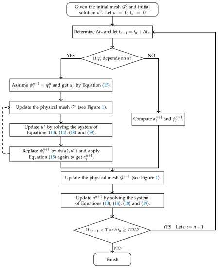
4. Numerical Examples and Discussion

Some numerical examples are presented in this section to verify the convergence rate, and to illustrate the accuracy and the efficiency of the proposed algorithm (see Figure 2). The solution behavior for various motions of heat sources are also investigated.

Example 1.

We consider a nonlinear moving interface problem with the exact solution

$$\begin{array}{c}\hfill u(x,t)=\left\{\begin{array}{cc}sin\left({\omega }_{1}x\right)e^{-{\omega }_1^{2}t},\hfill & x\le {\alpha }_0\left(t\right),\hfill \\ sin\left({\omega }_2(1-x)\right)e^{-{\omega }_2^{2}t},\hfill & x\ge {\alpha }_0\left(t\right),\hfill \end{array}\right.\end{array}$$

(20)

for some choice of ${\omega }_1$ and ${\omega }_2$. The interface ${\alpha }_0\left(t\right)$ is determined by solving the scalar equation

$$sin\left({\omega }_1{\alpha }_0\right)e^{-{\omega }_1^{2}t}=sin\left({\omega }_2(1-{\alpha }_0)\right)e^{-{\omega }_2^{2}t},$$

(21)

so that $u(x,t)$ is continuous across the interface.

Equation (21) has a unique solution [1] on the physical domain $[0,1]$ if ${\omega }_1=5\pi /4$ and ${\omega }_2=7\pi /4$, in which case, one has the initial interface position ${\alpha }_0\left(0\right)\approx 0.58333$ and the motion of the interface satisfies the ordinary differential equation

$$\begin{array}{c}\hfill \frac{\mathrm{d}{\alpha }_0}{\mathrm{d}t}=\frac{({\omega }_1^2-{\omega }_2^2)u({\alpha }_0,t)}{u_x({\alpha }_0^{-},t)-u_x({\alpha }_0^{+},t)}.\end{array}$$

(22)

Based on the jump conditions, the source function $F_0\left(u(x,t)\right)$ is

$$\begin{array}{cc}\hfill F_0\left(u(x,t)\right)& =-{\left[u_x\right]}_{{\alpha }_0}=u_x({\alpha }_0^{-},t)-u_x({\alpha }_0^{+},t)\hfill \\ & ={\omega }_{1}cos\left({\omega }_1{\alpha }_0\right)e^{-{\omega }_1^{2}t}+{\omega }_{2}cos\left({\omega }_2(1-{\alpha }_0)\right)e^{-{\omega }_2^{2}t}.\hfill \end{array}$$

(23)

The monitor function used to generate the adaptive mesh in MMPDE6 (5) is taken as

$$M(x,t)=(1-\theta )\left|\frac{\partial u}{\partial x}\right|+\theta {({(x-{\alpha }_0\left(t\right))}^2+\epsilon )}^{-1/4},$$

(24)

where $\theta =0.5$, $\epsilon ={10}^3/N^4$, and $\tau$ in MMPDE6 is set to be ${10}^{-3}$. In practical simulations, the monitor function is usually replaced by a smoother one [27] as

$${\tilde{M}}_i=\tilde{M}(x_i,t)=\sqrt{\sum _{k=i-\nu }^{i+\nu }{\left(M_k\right)}^2{\left(\frac{\gamma }{1+\gamma }\right)}^{|k-i|}/\sum _{k=i-\nu }^{i+\nu }{\left(\frac{\gamma }{1+\gamma }\right)}^{|k-i|}},$$

where $\gamma >0$ and $\nu \ge 0$ are two smoothing parameters, given by $\gamma =2$ and $\nu =2$ in the following experiments. The uniform time step size is set to be $\Delta t_n\equiv \frac{T}{L}$, and the termination time is taken as $T=0.1$.

Our goal is to verify the present algorithm has a second-order convergence rate for space. Because the exact solution is known, we simply employ Dirichlet boundary conditions $u(0,t)$ and $u(1,t)$ at the boundaries. The numerical results with different numbers of N and L at the time $T=0.1$ are listed in Table 1, where $E_N^d$ is the maximum error of u obtained from [8], and the other errors are defined by

$$\begin{array}{c}\hfill E_{N,L}^{\alpha }=\mid {\tilde{\alpha }}_0-{\alpha }_0^e\mid ,E_{N,L}^b=\parallel U_{N,L}-u^e{\parallel }_{\infty },E_{N,L}^c=\parallel {\tilde{U}}_{N,L}-u^e{\parallel }_{\infty },\end{array}$$

in which $u^e$ and ${\alpha }_0^e$ are the exact solutions of Equations (20) and (21) respectively (${\alpha }_0^e$ is obtained by the zero-finding MATLAB function fzero (MATLAB Release 2010a, The MathWorks, Inc., Natick, Massachusetts, MA, USA)). In addition, ${\tilde{\alpha }}_0$ is the solution of Equation (15) by one step of the predictor–corrector iteration. The numerical solutions U and $\tilde{U}$ are obtained by the algorithm shown in Figure 2 with ${\alpha }_0^e$ and ${\tilde{\alpha }}_0$, respectively. The ratio is defined as the error in the coarse mesh divided by the one in the finer mesh. The first two columns in Table 1 show that ${\tilde{\alpha }}_0$ is a good approximation of the exact solution ${\alpha }_0^e$, although we only adopt one step of the predictor–corrector iteration. Moreover, there is no remarkable difference between U and $\tilde{U}$. Both of them are better than those obtained in [8]. Finally, the numerical results illustrate that the convergence rate is second order in space.

Table 1. Error and convergence rate at $T=0.1$.

N, L	${\mathit{E}}_{\mathit{N},\mathit{L}}^{\mathit{\alpha }}$	Ratio	${\mathit{E}}_{\mathit{N},\mathit{L}}^{\mathit{b}}$	Ratio	${\mathit{E}}_{\mathit{N},\mathit{L}}^{\mathit{c}}$	Ratio	${\mathit{E}}_{\mathit{N}}^{\mathit{d}}$	Ratio
40, 40	8.2720 × ${10}^{-3}$	-	1.0931 × ${10}^{-2}$	-	1.3721 × ${10}^{-2}$	-	6.5460 × ${10}^{-3}$	-
80, 160	2.0540 × ${10}^{-3}$	4.0274	2.6996 × ${10}^{-3}$	4.0491	3.3908 × ${10}^{-3}$	4.0465	6.0108 × ${10}^{-3}$	1.0890
160, 640	5.1038 × ${10}^{-4}$	4.0245	6.6945 × ${10}^{-4}$	4.0326	8.4144 × ${10}^{-4}$	4.0297	1.1557 × ${10}^{-3}$	5.2009
320, 2560	1.2732 × ${10}^{-4}$	4.0085	1.6687 × ${10}^{-4}$	4.0117	2.0981 × ${10}^{-4}$	4.0104	2.9347 × ${10}^{-4}$	3.9381
640, 10,240	3.1807 × ${10}^{-5}$	4.0029	4.1678 × ${10}^{-5}$	4.0038	5.2408 × ${10}^{-5}$	4.0035	7.3175 × ${10}^{-5}$	4.0106
1280, 40,960	7.9500 × ${10}^{-6}$	4.0010	1.0416 × ${10}^{-5}$	4.0013	1.3098 × ${10}^{-5}$	4.0011	1.8237 × ${10}^{-5}$	4.0124
2560, 163,840	1.9874 × ${10}^{-6}$	4.0003	2.6038 × ${10}^{-6}$	4.0003	3.2743 × ${10}^{-6}$	4.0003	4.5462 × ${10}^{-6}$	4.0115

Figure 3 shows the evolution of the mesh and the solution profiles for Problems (20) and (21) with $N=24$. From the middle and the right subgraphs of Figure 3, it can be observed that the numerical solution (the solid line) are almost the same as the exact solution (the dots) at six different time stages $t=0,0.02,0.04,0.06,0.08,0.1$.

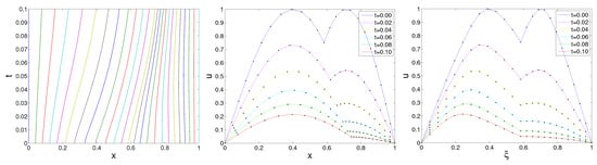
Figure 3. Mesh trajectories (left), the profiles of u in terms of x (middle) and $\xi$ (right) with $N=24$. The solid lines are the numerical solution and the dots are the exact solution.

The following examples are from moving source problems whose solutions may be blow-up [20,21,22]. The physical domain is chosen as $[-10,10]$ with $u(-10,t)=u(10,t)=0$ if it is not specifically pointed out. The initial value is given by

$$\begin{array}{c}\hfill u(x,0)=\left\{\begin{array}{cc}{cos}^2(\pi x/2),\hfill & -1<x<1,\hfill \\ 0,\hfill & \mathrm{otherwise},\hfill \end{array}\right.\end{array}$$

(25)

and the source functions $F_i\left(u(x,t)\right)$ are specified by

$$F_i\left(u(x,t)\right)=1+u^2,i=0,1,\dots ,q-1.$$

(26)

The monitor function in MMPDE6 (5) reads

$$M(x,t)={\theta }_{q+1}{u}^p+{\theta }_q\left|\frac{\partial u}{\partial x}\right|+\sum _{i=0}^{q-1}{\theta }_i{({(x-{\alpha }_i\left(t\right))}^2+\epsilon )}^{-1/4},$$

(27)

where $\epsilon \in (0,1]$, $p>0$, ${\theta }_i\in (0,1)$ and ${\sum }_{i=0}^{q+1}{\theta }_i=1$. The time step is chosen such that [20,28]

$$\Delta t_n=t_{n+1}-t_n=min\left\{\mu ,\frac{\mu }{{\left({max}_j\left\{u_j^n\right\}+\epsilon \right)}^2}\right\},$$

where $\mu ={10}^{-3}$. Additionally, the Newton iteration method is adopted to solve the resulting nonlinear system with the tolerance $tol={10}^{-8}$.

Example 2

(Linear moving sources). We consider that all sources move with a constant velocity k,

$${\alpha }_i^{\prime }\left(t\right)=k,{\alpha }_i\left(0\right)=d_i,i=0,1,\dots ,q-1,$$

where $d_0=0<d_1<\cdots <d_{q-1}$ are the positive constants.

Since the proposed algorithm is trivial for the problem with multiple sources, only numerical results for $q=1,2$ are presented here. In these cases, the solution phenomenon with $k=1,2$ has been investigated in [20,21,22]. Our numerical results give a satisfactory agreement with those shown in [20,21,22]. In more detail, the blow-up occurs with $k=1$, but it is avoided with $k=2$ in the case of $q=1$. The evolution of the moving mesh and the solution profiles in the case of $k=2$ and $q=1$ can be found in Figure 4, where the simulation parameters are given by $\tau ={10}^{-3}$, ${\theta }_0=0.9$, ${\theta }_1=0.1$, and $\epsilon ={10}^3/N^4$. Now let us add another heat source with $d_1=2.5$ and $k=2$; then, the phenomenon of blow-up can be observed again. With the simulation parameters $\tau =5\times {10}^{-4}$, ${\theta }_0={\theta }_1=0.3$, ${\theta }_3=0.4$, $p=2$, and $\epsilon ={10}^{-5}$, it is shown from Figure 5 that the blow-up occurs at the position of the first source, i.e., $x=4.079417297361286$, with the maximum value $u_{max}=3.16\times {10}^6$, and the corresponding blow-up time is $2.039708648680643$. This result is very close to the one obtained in [22], where the blow-up time for this case is 2.039311846765550.

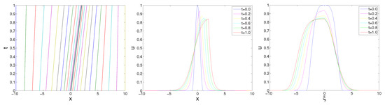
Figure 4. Mesh trajectories and the profiles of u from $t=0$ to $t=1.0$ for one source case with $N=100$.

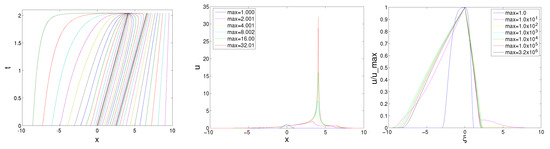
Figure 5. Mesh trajectories and the profiles of u with $N=150$ in the case of two sources.

The blow-up phenomena of the solutions in terms of $d_1$ for the two sources case are also investigated. Since the blow-up occurs in two sources case while it is avoided in one source case when $k=2$, it is expected that the blow-up time will be delayed as the distance $d_1$ increases, and there exists a critical distance, such that the blow-up does certainly occur if $d_1$ is less than the critical distance, while the blow-up will be avoided if $d_1$ is larger than the critical distance. As shown in Table 2, the blow-up time is delayed as expected as $d_1$ increases, yet the blow-up will still be observed even for $d_1=100$ when $k=2$. However, it can be seen that, in the case $d_1\ge 0.85$ for $k=3$ and $d_1\ge 0.04$ for $k=4$, the blow-up is avoided and the maximum of the solution $u_{max}$ would converge to the value listed in Table 2 as time evolves. A further computation using $N=1500$ shows that the critical distance for $k=4$ is between 0.03902 and 0.03903.

Table 2. Blow-up phenomena in terms of $d_1$ and k with $N=600$. The domain is $[x_l\left(t\right),x_r\left(t\right)]=[-{\alpha }_1\left(t\right),2{\alpha }_1\left(t\right)]$ for $k=2$, and $[x_l\left(t\right),x_r\left(t\right)]=[-{\alpha }_1\left(t\right)-5,2{\alpha }_1\left(t\right)+5]$ for others.

$\mathit{k}=2$			$\mathit{k}=3$			$\mathit{k}=4$
$2.5$	2.03881627	$3.16\times {10}^6$	$0.25$	1.14555847	$3.16\times {10}^6$	$0.01$	0.48168300	$3.16\times {10}^6$
5	3.10495654	$3.16\times {10}^6$	$0.5$	3.49923032	$3.16\times {10}^6$	$0.02$	0.61947967	$3.16\times {10}^6$
10	5.21961249	$3.16\times {10}^6$	$0.75$	10.60946467	$3.16\times {10}^6$	$0.03$	0.88168884	$3.16\times {10}^6$
25	11.64283736	$3.16\times {10}^6$	$0.8$	16.52257933	$3.16\times {10}^6$	$0.04$	-	0.78709834
50	22.56509042	$3.16\times {10}^6$	$0.85$	-	1.40807506	$0.05$	-	0.76986615
100	44.58805080	$3.16\times {10}^6$	$1.0$	-	1.26522313	$0.1$	-	0.71490192

Example 3

(Sin-type moving sources). We now consider the case of two sources, in which the sources move periodically with the same speed

$${\alpha }_0^{\prime }\left(t\right)={\alpha }_1^{\prime }\left(t\right)=Acos\left(\pi t\right),{\alpha }_0\left(0\right)=0,{\alpha }_1\left(0\right)=2.5.$$

For periodically moving sources, only one source case has been studied in [21]. Our numerical results are shown in Figure 6 for $A=\pi$. The simulation parameters are the same as those in Example 2. It is shown that the blow-up occurs at the location of the second source with the maximum value $u_{max}=3.16\times {10}^6$, and the corresponding blow-up time is $1.689611393639939$. This result is also very close to the one obtained in [22], where the blow-up time for this case is $1.688671486061044$.

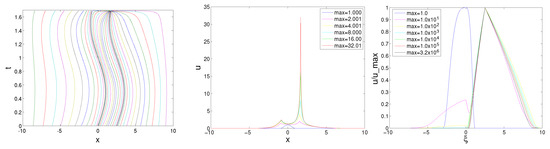
Figure 6. Mesh trajectories and the profiles of u for $q=2$, $A=\pi$ with $N=150$.

Example 4

(Symmetrically periodically moving sources). We consider the case of two sources, which move periodically and symmetrically. The motions are described by

$${\alpha }_0^{\prime }\left(t\right)=Acos\left(\pi t\right),{\alpha }_0\left(0\right)=-2.0,{\alpha }_1\left(t\right)=-{\alpha }_0\left(t\right),$$

where $A=\pi$.

To the best of my knowledge, there are no theoretical and numerical results for multiple sources with different speeds at present. For the two sources moving periodically and symmetrically, it is anticipated that if the blow-up occurs, then it occurs at the locations of both sources at the same time. However, it is difficult to simulate this symmetrical blow-up phenomenon due to numerical perturbation. Indeed, the globally moving mesh strategies proposed in [20,21] usually fail to capture the symmetrical blow-up phenomenon. However, with the benefit of the domain-decomposed adaptive mesh generation, one can simulate this symmetrical blow-up phenomenon very well. As shown in Figure 7, the blow-up occurs as expected at the locations of both sources in the time $2.496881990359248$, where the maximum value of the solution is $u_{max}=3.16\times {10}^6$. For a comparison, we also present the simulation results with LABCs (17) on a much smaller physical domain $[{\alpha }_0\left(t\right)-4.0,{\alpha }_1\left(t\right)+4.0]$ in Figure 8. It can be seen that the blow-up time $2.496370241342059$ is very close to that in Figure 7, which shows the effectiveness of the LABCs. That is, a smaller physical domain with LABCs, indicating smaller computational cost, can be employed in the numerical investigation of the moving heat sources’ problems.

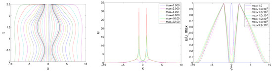
Figure 7. Numerical results for symmetrically periodically moving sources with $N=150$.

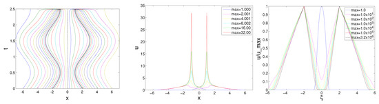
Figure 8. Numerical results for symmetrically periodically moving sources with $[x_l,x_r]=[{\alpha }_0\left(t\right)-4.0,{\alpha }_1\left(t\right)+4.0]$.

5. Conclusions

A domain-decomposed moving mesh method has been developed for the heat conduction problem with multiple localized sources, which can be moving with different speeds. The special adaptive moving mesh can be generated very efficiently by parallel computing, and the discretization of the model equation on it is simplified a lot without loss of accuracy. A predictor–corrector algorithm is proposed to capture the trajectories of the heat sources and the solution of the model equation accurately. To the best of my knowledge, this is the first time to investigate the solution phenomenon for the problem of multiple heat sources with different speeds. With the proposed method, we have investigated the dependence of the solution on the moving sources such as the types of motion and the distance between sources. The symmetrical blow-up phenomenon in the case that two sources are moving symmetrically and periodically is also successfully simulated.

Finally, the derived discretization of the underlying equation is reinterpreted from a new point of view, which shows that the same discretization can also be derived by first replacing the delta function with a mesh-dependent hat function, and then applying standard numerical methods to the resulting equation. Since the jumps of solution are completely avoided in the new approach, one may extend the present method to multi-dimensional problems with moving localized heat sources. Actually, this work is ongoing and would be reported elsewhere soon. For the case that the moving localized heat sources may be crossing with other sources, it is obvious that the domain-decomposed moving mesh method could not be applied directly. However, the idea, approximating the delta function by a mesh-dependent hat function, may still work and give an accurate discretization, which will be considered in my future work.

References

- Beyer, R.P.; LeVeque, R.J. Analysis of a one-dimensional model for the immersed boundary method. SIAM J. Numer. Anal. 1992, 29, 332–364. [Google Scholar] [CrossRef]
- Mirkoohi, E.; Ning, J.; Bocchini, P.; Fergani, O.; Chiang, K.N.; Liang, S.Y. Thermal modeling of temperature distribution in metal additive manufacturing considering effects of build layers, latent heat, and temperature-sensitivity of material properties. J. Manuf. Mater. Process. 2018, 2, 63. [Google Scholar] [CrossRef]
- Ma, J.; Sun, Y.; Yang, J. Analytical solution of dual-phase-lag heat conduction in a finite medium subjected to a moving heat source. Int. J. Therm. Sci. 2018, 125, 34–43. [Google Scholar] [CrossRef]
- Sun, Y.; Liu, S.; Rao, Z.; Li, Y.; Yang, J. Thermodynamic response of beams on Winkler foundation irradiated by moving laser pulses. Symmetry 2018, 10, 328. [Google Scholar] [CrossRef]
- Reséndiz-Flores, E.O.; Saucedo-Zendejo, F.R. Two-dimensional numerical simulation of heat transfer with moving heat source in welding using the Finite Pointset Method. Int. J. Heat Mass Transf. 2015, 90, 239–245. [Google Scholar] [CrossRef]
- Kirk, C.M.; Olmstead, W.E. The influence of two moving heat sources on blow-up in a reactive-diffusive medium. Zeitschrift für Angewandte Mathematik und Physik 2000, 51, 1–16. [Google Scholar] [CrossRef]
- Kirk, C.M.; Olmstead, W.E. Blow-up in a reactive-diffusive medium with a moving heat source. Zeitschrift für angewandte Mathematik und Physik 2002, 53, 147–159. [Google Scholar] [CrossRef]
- Li, Z. Immersed interface methods for moving interface problems. Numer. Algorithms 1997, 14, 269–293. [Google Scholar] [CrossRef]
- Budd, C.J.; Huang, W.; Russell, R.D. Moving mesh methods for problems with blow-up. SIAM J. Sci. Comput. 1996, 17, 305–327. [Google Scholar] [CrossRef]
- Huang, W.; Ma, J.; Russell, R.D. A study of moving mesh PDE methods for numerical simulation of blow-up in reaction diffusion equations. J. Comput. Phys. 2008, 227, 6532–6552. [Google Scholar] [CrossRef]
- Hu, Z.; Wang, H. A moving mesh method for kinetic/hydrodynamic coupling. Adv. Appl. Math. Mech. 2012, 4, 685–702. [Google Scholar] [CrossRef]
- Cheng, J.B.; Huang, W.; Jiang, S.; Tian, B. A third-order moving mesh cell-centered scheme for one-dimensional elastic-plastic flows. J. Comput. Phys. 2017, 349, 137–153. [Google Scholar] [CrossRef]
- Lu, C.; Huang, W.; Qiu, J. An adaptive moving mesh finite element solution of the regularized long wave equation. J. Sci. Comput. 2018, 74, 122–144. [Google Scholar] [CrossRef]
- Zhang, F.; Huang, W.; Li, X.; Zhang, S. Moving mesh finite element simulation for phase-field modeling of brittle fracture and convergence of Newton’s iteration. J. Comput. Phys. 2018, 356, 127–149. [Google Scholar] [CrossRef]
- Huang, W.; Ren, Y.; Russell, R.D. Moving mesh partial differential equations (MMPDES) based on the equidistribution principle. SIAM J. Numer. Anal. 1994, 31, 709–730. [Google Scholar] [CrossRef]
- Huang, W.Z.; Russell, R.D. Adaptive Moving Mesh Methods; Springer Science & Business Media: Berlin, Germany, 2011. [Google Scholar]
- Haynes, R.D.; Russell, R.D. A Schwarz waveform moving mesh method. SIAM J. Sci. Comput. 2007, 29, 656–673. [Google Scholar] [CrossRef]
- Gander, M.J.; Haynes, R.D. Domain decomposition approaches for mesh generation via the equidistribution principle. SIAM J. Numer. Anal. 2012, 50, 2111–2135. [Google Scholar] [CrossRef]
- Haynes, R.D.; Kwok, F. Discrete analysis of domain decomposition approaches for mesh generation via the equidistribution principle. Math. Comput. 2017, 86, 233–273. [Google Scholar] [CrossRef]
- Ma, J.; Jiang, Y. Moving mesh methods for blow-up in reaction-diffusion equations with traveling heat source. J. Comput. Phys. 2009, 228, 6977–6990. [Google Scholar] [CrossRef]
- Zhu, H.; Liang, K.; Cheng, X. A numerical investigation of blow-up in reaction-diffusion problems with traveling heat sources. J. Comput. Appl. Math. 2010, 234, 3332–3343. [Google Scholar] [CrossRef]
- Hu, Z.; Wang, H. A moving mesh method for heat equation with traveling singular sources. Appl. Math. J. Chin. Univ. Ser. A 2013, 28, 115–126. (In Chinese) [Google Scholar]
- Toselli, A.; Widlund, O.B. Domain Decomposition Methods—Algorithms and Theory; Spinger: Berlin, Germany, 2005. [Google Scholar]
- Peskin, C.S. Numerical analysis of blood flow in the heart. J. Comput. Phys. 1977, 25, 220–252. [Google Scholar] [CrossRef]
- Hu, Z. Moving Mesh Method and Its Applicatios Coupled with Dynamic Domain Decomposition. Ph.D. Thesis, Zhejiang University, Hangzhou, China, 2012. (In Chinese). [Google Scholar]
- Brunner, H.; Wu, X.; Zhang, J. Computational solution of blow-up problems for semilinear parabolic PDEs on unbounded domains. SIAM J. Sci. Comput. 2010, 31, 4478–4496. [Google Scholar] [CrossRef]
- Huang, W.; Ren, Y.; Russell, R.D. Moving mesh methods based on moving mesh partial differential equations. J. Comput. Phys. 1994, 113, 279–290. [Google Scholar] [CrossRef]
- Budd, C.J.; Leimkuhler, B.; Piggott, M.D. Scaling invariance and adaptivity. Appl. Numer. Math. 2001, 39, 261–288. [Google Scholar] [CrossRef]
© 2018 by the author. Licensee MDPI, Basel, Switzerland. This article is an open access article distributed under the terms and conditions of the Creative Commons Attribution (CC BY) license (http://creativecommons.org/licenses/by/4.0/).