Article

Comparison of Random Subspace and Voting Ensemble Machine Learning Methods for Face Recognition

1
Institute for Analysis and Scientific Computing, Vienna University of Technology, Vienna 1040, Austria
2
College of Engineering, Effat University, Jeddah 21478, Saudi Arabia
*
Author to whom correspondence should be addressed.
Symmetry 2018, 10(11), 651; https://doi.org/10.3390/sym10110651
Submission received: 9 October 2018 / Revised: 12 November 2018 / Accepted: 14 November 2018 / Published: 19 November 2018

Abstract

:
Biometry based authentication and recognition have attracted greater attention due to numerous applications for security-conscious societies, since biometrics brings accurate and consistent identification. Face biometry possesses the merits of low intrusiveness and high precision. Despite the presence of several biometric methods, like iris scan, fingerprints, and hand geometry, the most effective and broadly utilized method is face recognition, because it is reasonable, natural, and non-intrusive. Face recognition is a part of the pattern recognition that is applied for identifying or authenticating a person that is extracted from a digital image or a video automatically. Moreover, current innovations in big data analysis, cloud computing, social networks, and machine learning have allowed for a straightforward understanding of how different challenging issues in face recognition might be solved. Effective face recognition in the enormous data concept is a crucial and challenging task. This study develops an intelligent face recognition framework that recognizes faces through efficient ensemble learning techniques, which are Random Subspace and Voting, in order to improve the performance of biometric systems. Furthermore, several methods including skin color detection, histogram feature extraction, and ensemble learner-based face recognition are presented. The proposed framework, which has a symmetric structure, is found to have high potential for biometrics. Hence, the proposed framework utilizing histogram feature extraction with Random Subspace and Voting ensemble learners have presented their superiority over two different databases as compared with state-of-art face recognition. This proposed method has reached an accuracy of 99.25% with random forest, combined with both ensemble learners on the FERET face database.

1. Introduction

1.1. Background

In this era, the reliability of real-time personal identification in different applications is a crucial issue. Human beings have unique inborn features that distinguish them from other creatures. Biometric systems, being a part of information technologies, is a discipline which works on authentication by extracting hints to identify a person, such as examining people’s physical features and ways of behavior. Retina recognition, hand and vein recognition, iris recognition, face recognition, and fingerprint recognition can be counted as some of the most frequently used physical recognition methods. Features like a fingerprint, palm print, and iris scan are some of the most distinct ones that enable human beings to be distinguished. Biometric technology, which performs identification by using these characteristic features, has been used for security and authentication reasons in recent years. Although biometric identification systems can eliminate the limitations relevant to the use of passwords, they are vulnerable to spoofing attacks [1,2]. Gait and keystroke identification techniques are not very secure with regard to identification accuracy. Similarly, a voice feature that might be imitated, or a fingerprint that might be falsified by a gummy fingerprint, or an iris that might be duplicated by using contact lenses, are also not robust against falsifications [3].

1.2. Research Motivations

Computers can visualize vast amounts of information, and this was the basis for biometrics advancements such as face recognition, vein geometry, hand geometry, etc. Several professionals have researched face recognition, as it is not expensive and it is non-intrusive. This system has three stages by which it functions. The first one is face detection, followed by feature extraction and after that, face recognition. A comparison of faces in order to establish the requested identity is the authentication part of the procedure. Identification, on the other side, compares the identity to a few different face possibilities. [4]
Face recognition has been showing incredible advancements in the last 20 years, and it has been shown to be practical in a number of different areas, such as commercial and law-enforcement areas. There have been numerous advancements in different areas, such as social networks, which fostered an improvement in law enforcement databases that have allowed for impactful applications in areas such as face tagging, and this has been applied in areas such as mug shot matching, finding missing persons, etc. In a face recognition system that uses cloud services, the face recognition engine can be found in the cloud, but it cannot be found in the local processing area. In an application that has been used in commercial applications following the client–server model, the user takes the sample face image, and it is moved to the cloud in order to be able to conduct authentication from the gallery, using face recognition that could be found on the cloud [5].
Over the past few years, researchers have made contributions to classification and extraction with some different methods [6]. There are two essential matters regarding the planning of a face recognition framework. These are feature extraction and classifier structure. In the past few decades, different feature extraction methods or methods that reduce the size were offered, to match a high-dimensional sample with a lower-dimensional sample [7]. In recent decades, the demand for face recognition in different security areas has helped the police to shortlist potential criminals. Studies indicate that the face recognition applications show excellent efficiency with such complicated tasks [8]. Different approaches are proposed in solving the problem with this method. In the constrained scenes, such as airport scanners or ATM cash withdrawal, a frontal image is captured, which is quite straightforward, and it is different from the context in which the scene is not constrained [9].
Nevertheless, the selection of the classifier is essential when it comes to problems of face recognition, and solving such problems. Ensemble learning has its composition being made of different classifiers. Ensemble learning algorithms have also been employed in face recognition [10,11,12,13,14]. In trying to create an efficient and effective system, there is a need for efficient computing methods and techniques that have increased classification accuracy [12]. Hence, the research aim of this paper is to employ and compare ensemble classifiers in face recognition.

1.3. Contribution

Based on the above-mentioned motivations, a new face recognition model based on a simple feature extraction method, i.e. histogram and ensemble classifiers, are proposed, with the aim to increase the accuracy and to have better classification performance. Single classifiers such as k-Nearest Neighbor (k-NN) and Artificial Neural Network (ANN) cannot deal with high-dimensional data without variable selection or dimension reduction, whereas SVM can classify high-dimensional data, but it is not robust to the existence of a significant number of irrelevant variables. In order to eliminate these types of problems, there is a need for face recognition, to introduce more efficient machine learning techniques; these can particularly achieve a much better performance. In this study, to eliminate the limitations above, the use of a combination of a histogram feature extraction with the ensemble classifier framework for the face recognition is proposed. In particular, this paper compares the Random Subspace and Voting ensemble classifiers to improve generalized (testing) classification performances. Random Subspace is also employed by Bashbaghi et al. [13] for face recognition, but the performance comparison of Random Subspace and Voting using several classifiers by utilizing histogram feature extraction for face recognition has not been realized yet.

1.4. Organization

The rest of this paper is organized as follows. The literature is reviewed in Section 2. Databases, the general design of the proposed system, and learning methods used are presented in Section 3. Section 4 explains the experimental methodology—protocol, experimental setup, utilized databases, and measures applied in performance evaluation. Moreover, the comparison of the performances of the proposed algorithm with other state-of-the-art classifiers is presented in Section 4 as well. Lastly, Section 5 expresses the conclusion.

2. Literature Review

Face biometry has many benefits that have been gained from machine learning, compared to the other biometrics. The main focus of this method is the pre-processing stage, which includes face detection and facial features extraction. Face recognition is essentially a classification problem [14].
A face recognition system has been proposed to utilize the AdaBoost [15]. This method examines the redundancy among classifiers candidates, and then makes a selection. This method also utilized the Gabor feature selection for face recognition on the FERET database. Zong and Huang [16] researched the efficiency of the one-against-all and one-against-one extreme learning machine (ELM) for classification in multi-class face recognition problems. Kremic et al. [17] proposed a client–server model and compared it with the newest client–server models for face recognition with a design that applies a security private key to transfer the images over the network securely. Vinay et al. [5] developed a face recognition framework through the ideas of cloud Computing, big data, social networks, and machine learning, to execute the duty of face tagging for social networks operating on big data.
Wang et al. [12] introduced a new face recognition method working on discriminant tensor subspace analysis and ELM. De-la-Torre et al. [18] proposed new adaptive multiple classifier structures for partly-supervised learning of facial prototypes shift working on facial lines. Li et al. [7] proposed a framework to utilize a radial basis function neural network to obtain knowledge on the feature extraction operation of kernel subspace techniques. Han et al. [19] offered a new Incremental Boosting Convolutional Neural Network (CNN) to supplement boosting into the CNN through an incremental boosting layer that chooses discriminative neurons from the lower layer, and is hierarchically updated on successive mini-batches. Zhao et al. [8] offered a super-resolution reconstruction method by adaptive multi-dictionary learning, and compared it with the traditional global dictionary learning, which uses less time on dictionary training and image rebuilding to a high level. Dai et al. [10] used neural networks with random weights to apply such learning structures to the face recognition field.
Kremic and Subasi [20] compared the random forest (RF) with the Support Vector Machine (SVM). Principal component analysis (PCA) with a feature vector extraction method was applied for face recognition. Zhao et al. [21] proposed a new neural network method, called a low-rank-recovery network, to overcome the problems mainly affected by matrix completion and deep learning methods. Kim et al. [22] developed a face recognition framework through symmetrical fuzzy-based quality assessment. Wang et al. [23] employed two novel features for face liveness recognition schemes, to protect against replayed attacks and printed photo attacks for the biometric authentication scheme.
Li et al. [24] developed a face recognition framework employing facial-aided in-depth learning features of the texture feature. In the proposed framework, features are extracted from the mouth, nose, and eyes area. Then, extracted features are utilized with in-depth learning features to adaptively tune the deep learning parameters and to achieve enhanced face recognition accuracy. Yang et al [25] developed a novel multimodal biometrics recognition model based on the canonical correlation analysis (CCA) and stacked extreme learning machines. They used the FERET and ORL face databases. Sajid et al. [26] extracted facial-asymmetry-based demographic informative features to evaluate the age group, gender, and race of a given face image by employing two well-known face datasets, MORPH II and FERET. Wang et al. [27] proposed the deep learning technique to obtain facial landmark detection and limitless face recognition. To overcome the face landmark detection issue, they offered a layer-by-layer training technique of a deep convolutional neural network.

3. Materials and Methods
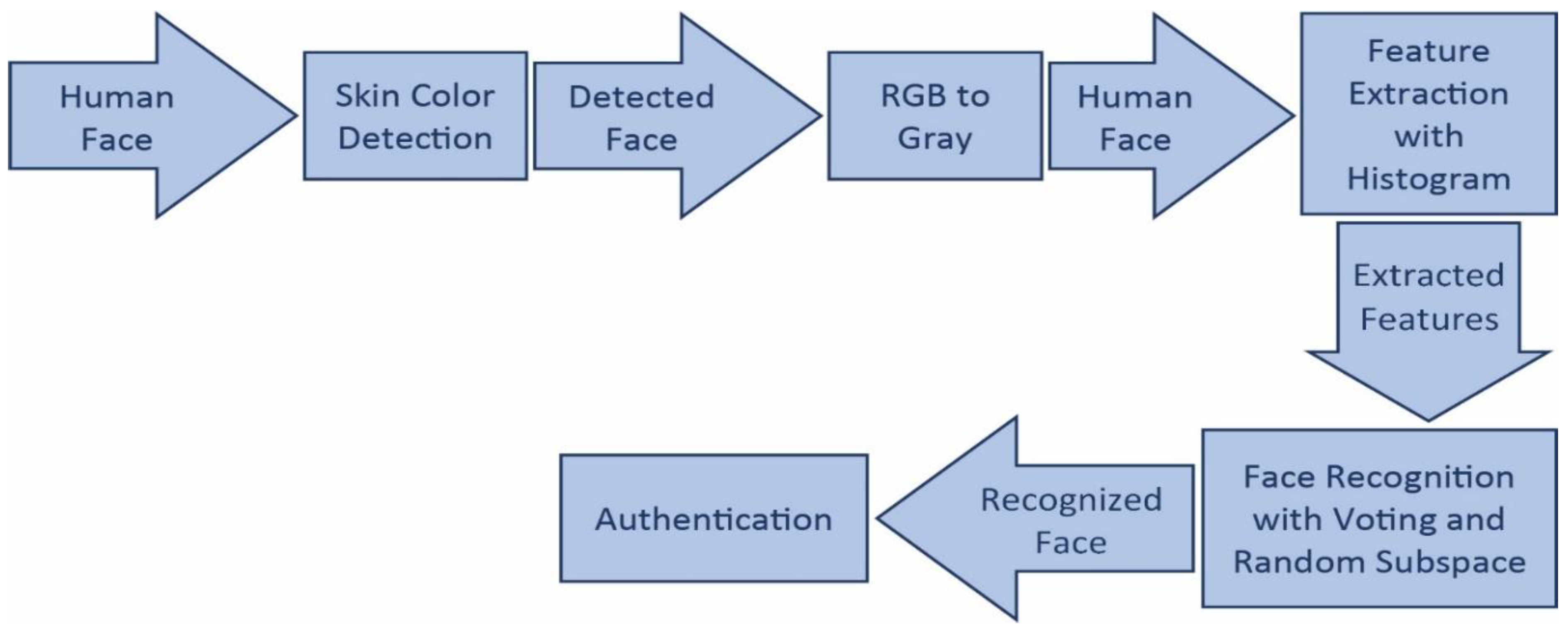
Face recognition has been very appealing to the scientific community within the last few decades. Several improvements in this area are needed in some different systems, from commercial areas to justice areas. Face recognition is not invited, and face recognition can be conducted without the physical interaction of the subject. Even so humans can easily recognize faces, which is inherent to human beings, while computerized face recognition is very demanding, as faces are not standardized geometric figures and cannot be interpreted as such. Now the advantage in this sense is that computer-based face recognition allows the process to handle various faces, while there is a limitation to the recognition of faces due to human memory. Although every human has different face characteristics, the human can easily differentiate and identify faces. Alterations in hair from ageing, lighting, outlook variations, and changes of the background are the primary difficulties that are handled by an automatic face recognition application. There are three subtasks when it comes to the automatization of face recognition. First is face detection, then the feature extraction, and the last one is identification. In the past, the problem in this segment has been done in different ways. There were cases in which researchers used localized faces in classification and feature extraction. On the other side, few schemes isolate different tasks in order to achieve greater simplifications of face recognition, and this fosters the assessment and advancement of different parts of methods. The usage of the placed face section enhances accuracy in classification, although an extra section is needed, which increasing the difficulty of the computations. When the localization of faces is done, the recognition is simplified to background clutter, and incorrect data is removed. The algorithm can be tested in such a way that databases are applied without earlier localization, and then the center of interest is now focused on developing new and effective feature extraction methods [28].

3.1. Face Detection

The face detection aims to determine whether a sample in a photo or the video contains a face or not. Actually, this is very challenging, based on a few factors. Firstly, there are so many characteristics of a face in the range from color to size. Second, faces have different shapes. Besides that, it is placed in an environment that can be very different and demanding. Hence, in order to identify a face, one must use different approaches. Viola and Jones are used as an algorithm for face detection. Now, when a raw or filtered image is an input for a classifier, the space dimension is quite significant. In order to be efficient, extrapolation must be made from a certain amount of training samples [29]. The human skin could also be an attractive feature, despite different colours and shapes; the difference is made based on intensity rather than chrominance [30].

3.2. Facial Feature Extraction

There are different methods of facial feature extraction. Different samples are used for automatization, for different reasons. Samples are taken using different sensors. Features are used throughout the process. This extraction can be easily compared to the human brain process, which identifies human faces with an approach named feature extraction. The perception method of the human brain is in the form of separating the human face into its eyebrows, eyes, nose, and lips, and identifying these vectorially. It is impossible to capture the whole process of how the human brain recognizes images [31]. From that process, the criteria for identification can be the basis of face recognition applications. Particular characteristics of a face or different parts are the segments of a face by which the recognition is based. Techniques include focusing on binary pattern features. Discrete cosine transform-based features and Gabor wavelet transform-based features are the most widely used methods when compared to many other methods. The Local Binary Pattern was placed with the goal of designing efficient classification texture [32]. Local Binary Pattern histograms are derived from the face image, and then they are divided into a number of small areas; after that, they can be compiled in one histogram. The shape and texture of the samples in the recognition system are represented in that way. In this study, a simple feature extraction method which is a histogram, is proposed.

3.3. Face Recognition

The face recognition is one of the biometric systems. It is very functional, and it is used in the identification and authentication of an image or a video frame, since every face has its own special characteristics such as eye distance, nose characteristics, cheekbones, etc. These are represented within the database by numbers and are named as the faceprint [33].

3.4. Classification Methods

3.4.1. Artificial Neural Networks (ANN)

ANN include input/output units that are connected, and every connection has weight. This network adapts the weights to make it possible for a prediction of the right class label during learning. ANN can successfully tolerate and manage noisy data to make a proper classification of those patterns that are not familiar to it. Additionally, ANN produced the basis for the development of some other techniques, which are applicable in different areas. Backpropagation is the most common ANN method out of many kinds of artificial neural networks [34]. The best performance is achieved with a learning rate of 0.3 and a momentum value of 0.2, with 48 nodes in the hidden layer in the implementation of ANN.

3.4.2. k-Nearest Neighbor (k-NN)

The k-NN method is founded on analogy, as it compares training instances that are similar to the instances that are given to it. It uses n attributes to describe the training instance. Every instance is a point in n-dimensional space that makes an n-dimensional pattern space where every training tuple is saved. In a case where the unknown instance was assigned, a classifier seeks the known characteristics that are the most similar to the unknown instance. These are known as the k “nearest neighbors” to the instance that is unknown. In this situation, the k-nearest-neighbor examines whether among the patterns there is one that is similar to the unknown instance. In particular, pattern instances are known as k “nearest neighbo = rs” to the assigned unknown instances. How similar one tuple is to another is defined by sets of metrics, one of which is the Euclidean distance [34]. The best performance is achieved with a k value of 3 in the k-NN implementation.

3.4.3. Support Vector Machine (SVM)

The SVM is a classification algorithm that classifies nonlinear and linear data. Nonlinear mapping is used in transformation of original training data to a higher dimension. In the new dimension, it starts searching within that dimension for a linear optimal separating hyperplane, the segment that separates those instances from one class that are different from another class. Hyperplanes always separate data from different classes, with nonlinear mapping. This hyperplane is found by SVM using margins and support vectors [34]. The performance of the SVM classifier is mostly affected by the chosen kernel and the kernel parameters [35,36]. The best performance is achieved with a Puk kernel and with a kernel parameter C = 1 in the implementation of SVM.

3.4.4. Naïve Bayes (NB)

Naïve Bayes is a simple approach that can perform better than some other advanced classifiers. The idea behind this thought is that one should always try the simple way at the beginning. Attributes are managed as they were though and independent in their class. This might eventually be better; by including subgroups of features in the operation of decision making by making a comprehensive choice of attributes that will be used. The other restriction on Naïve Bayes can be done by normal-distribution assumption when using numeric attributes, as many features are not distributed normally [34].

3.4.5. Classification and Regression Tree (CART)

The CART is one of the decision tree learners that classifies with the employment of the pruning strategy, which is called the minimal cost-complexity. However, the CART learner and this strategy have only one similarity with the decision tree, and it is the name. With regard to the description of decision trees, assumedly, there is just one attribute that is used in splitting the data into subsets in every part of the tree. It is also possible to have the tests done by involving different parts of the same tree at the same time. Multivariate decision trees are those trees on which tests are done that involve a more significant number of attributes, with the simple ones being called univariate, and they are more frequently used than the multivariate trees. There is also the possibility to generate multivariate tests that can also be done by the CART system. These can often be much more accurate, and they can also be slightly smaller when compared to univariate trees, and they could also be much more consuming and take much more time to generate, and they are also tough to interpret [34]. The default parameters are used in the implementation.

3.4.6. C4.5 Decision Tree

The C4.5 decision tree algorithm tests for which training examples have the same result, are eliminated as they are not very important. Therefore, they are not contained in the decision tree if they do not have a minimum of two outcomes, which have a minimum number of instances. The given value for the minimum is 2, yet we can control it and raise it for tasks with noisy data. Candidate splits are taken into consideration in the case that they cut a specific number of instances. After the subtraction, we might find out that the information gain is negative. If we do not have attributes that have a positive information gain, which is a kind of pre-pruning, the tree will stop growing. This is indicated at this point, since it could be unexpected to obtain a pruned tree although post pruning is not active [37]. The default parameters are used in the implementation.

3.4.7. REP Tree

REPTree is a building decision, in other cases, a regression tree determined by the usage of information, which is in essence gain reduction, so it is a method of pruning with reduced errors. Optimization is done so it can be sped up, and only able to sort the values once in cases where numeric attributes are used. Like C4.5, it splits instances into different pieces. The minimum number of instances can be set per leaf [34]. The default parameters are used in the implementation.

3.4.8. AD Tree

Alternating decision trees (AD Trees) combine the weak hypotheses produced throughout boosting into a single explainable demonstration. The AD Tree is induced from AdaBoost. Three nodes are inserted to the tree at each iteration of boosting. A dividing node tries to divide groups of samples into two prediction nodes. Another attractive feature of AD Trees is their ability to be merged where it is not possible using conventional boosting procedures. This is a mainly beneficial attribute in the context of multiclass problems, since they are frequently re-formulated into the two-class setting [38]. The default parameters are used in the implementation.

3.4.9. LAD Tree

The Logical analysis of data trees (LAD Tree) utilizes the logistic boosting technique to create an alternative decision tree. A single attribute test is selected as a splitter node for the tree at every repetition. The predicted values are characterized by the vector that is the total result of all the ensemble classifiers on the instance over the classes. The LogitBoost algorithm can be merged with the induction of AD Trees, either by growing separate trees for each class in parallel, or only one tree is grown to predict all of the class possibilities at the same time [38]. The default parameters are used in the implementation.

3.4.10. Random Tree Classifiers

The random tree gathers some different learning algorithms as they collect a high number of particular learners. The idea behind this is a bagging idea, which produces a set of data without any particular preference, which is then used in the decision tree construction. When it comes to standard trees, every node is then divided by examining the different variables to reach the best possible split. In case of a so-called random forest, every node is divided by the usage of predictors; those predictors that are extracted from the whole subset at the particular node. The Random Tree Classifier uses the input feature vector, then it makes a classification of it to every tree that is in the forest, and then outputs the label of the class that was the most “voted” one. These model trees actually represent the decision trees in cases where the linear model that has gone through optimization is held in each of the leaves with the purpose of reaching the local subspace where the leaf presents it. The single decision trees have their performance enhanced by the usage of different possibilities of randomization, and also by the usage of tree diversity [37,39]. The default parameters are used in the implementation.

3.4.11. Random Forests (RF)

The decision tree forest is as a collective that is formed by tree classifiers that are built concerning random vectors. Random forests allow various schemes that are part of decision tree (DT) ensembles to act in example bagging, in cases where the abovementioned random vectors are directly related to them, with n being the elements number in training dataset, and object indices with a point to the elements that include a bootstrap sample. Various sources can be used to make the forest trees random. Such sources can be different configurations of DT. Breiman analyzed two different methods of the random feature selection for every DT using the CART algorithm that was mentioned and explained before [40]. The idea for this was to have more diversity when it comes to split selection and randomization. The procedure was done such that the best split was selected from some random splits, without the specifics in selecting the features to be split. This was done in a way so that no specific split was selected if there was no best individual split, but rather one attribute in all of the splits that kept popping out. Breiman [40] also used the random feature for one more advantage, that being the reduced cost of the computing that was required for DT inducing [41]. The best performance was achieved with a tree size of 100 in the implementation of RF.

3.4.12. Rotation Forest (RoF)

Rotation Forest (RoF) has a basis in the extraction of features. Training data is created in a way such that features are split and placed in subsets and PCA and then applied to every subgroup. There are also another concept that is called rotation, which encourages variety in the ensemble. This variety is maintained within the subtraction of features for every classification of the base. Because decision trees are so sensitive to the feature axis rotation, they were presented here and rightfully named a forest [42]. Conceptually, this approach is to foster both diversification and accuracy in the ensemble. This diversification is continued within the extraction of a feature in every base classification. These principal components are being held within accuracy, but also with the usage of the entirety of the dataset that is training every base classifier. There, we also have a learning method within the ensemble that is named a rotation forest, which incorporates a particular goal that creates diversification while also achieving accuracy within the classifiers. We have a combination of the Voting and Random Subspace methods that have principal components in the building and formation of the decision trees [37].

3.5. Ensemble Methods

Ensemble learning methods allow for the use of robust classifiers that are widely used in different pattern recognition areas. Recently, ensemble classifiers have increasingly gained more attention in different pattern recognition applications. The ensemble classifications that focus on the entirely complex-valued relaxation neural networks are applied to the classification of images. They apply multiple classifiers for the same classification problem. In this learning method, the results of classifiers with different accuracy scores are combined with different methods (voting, average, etc.). Thus, it is possible to obtain better predictive results from a single classifier [43]. There are several types of ensemble methods. In this study, we applied Random Subspace and Voting methods.

3.5.1. Random Subspace Method

The Random Subspace Method (RSM) is an ensemble classifier technique that is proposed by Ho [44]. In the RSM, the training data is modified. However, this data modification is carried out in the feature space. Hence, each training incidence Xi (i = 1, …, n) in the training sample set X = [X1; …; Xn] is defined as a p-dimensional vector Xi = (xi1, xi2, …, xip), defined by p features. Then, randomly r < p features from the p-dimensional data set X are selected. Consequently, the modified training set X b ˜ = X 1 b ˜ ,   X 2 b ˜ ,   X n b ˜ , is composed of r-dimensional training incidences. After this step, classifiers are built into the random subspaces X b ˜ and aggregated by utilizing a majority voting. Therefore, the RSM is implemented in the following way:
  • Repeat for b = 1, 2, …, B:
  • Choose an r-dimensional random subspace X b ˜ from the original p-dimensional feature space X.
  • Build a classifier Cb(x) (with a decision boundary Cb(x) = 0) in X b ˜ .
  • Aggregate classifiers Cb(x), b =1, 2, …, B, by utilizing majority voting for the final decision.
The RSM can benefit from using random subspaces for both building and combining the classifiers. When the number of training incidences is comparatively small as compared to the data dimension, by building classifiers in random subspaces, the small sample size problem can be solved. The subspace dimension will be less than the original feature space, while the number of training incidence is kept the same. Thus, the relative training sample size increases. Once the data have several redundant features, the better classifier can be found in random subspaces than in the original feature space. The aggregated decision of such classifiers might be better than a single classifier build on the original training set in the entire feature space [45].
There are parameters to be tuned for Random Subspace ensemble learning algorithms. After many experiments, the best results were achieved by applying the following values for parameters.
  • Classifier: represents the base classifier to be applied. We applied 11 different classifiers such as ANN, k-NN, SVM, RF, C4.5, Random Tree, REP Tree, LAD Tree, NB, Rotation Forest, and CART.
  • Numiterations: represents the number of repetitions to be applied. The best performance is achieved for a setting up to 10.
  • Seed: represents the number seed to be applied randomly. The best performance is achieved with a seed = 1 in the implementation of the random subspace.
  • Subspacesize: represents the size of each subspace. The best performance is achieved with a subspace = 0.5 in the implementation of the random subspace.

3.5.2. Voting

The Voting ensemble learning method is one of the simple methods to aggregate multiple classifiers. Voting involves obtaining a linear combination of learners.
y i = j w j d j i   where   w j 0 , j w j = 1
In a weighted sum, dji is the vote of classifier j for class Ci and wj is the weight of its vote. Simple voting is a special case in which all voters have equal weight, namely, wj = 1/L. This is known as plurality voting, in which the class taking the majority of votes is the winner. Moreover, if the voters provide the additional knowledge on how much they vote for each class, then after normalization, these might be employed as weights in a weighted voting system. Consistently, if dji is the class posterior probabilities, P(Ci|x, Mj), then they can be summed up (wj = 1/L) and the class with maximum yi will be selected. The median can be more robust to noise than the average. Another way might be to assess the accuracies of the learners on a distinct validation set, and to utilize that information to find the weights so that more weights can be given to more accurate learners [46].
There are parameters to be tuned for Voting ensemble learning algorithms. After many experiments, the best results were achieved by applying the following values for the parameters.
  • Classifier: represents the base classifier to be combined with default classifier. We applied 11 different classifiers such as ANN, k-NN, SVM, RF, C4.5, Random Tree, REP Tree, LAD Tree, NB, Rotation Forest, and CART.
  • Combinationrule: represents the combination rule to be applied. The best performance is achieved with an average of probabilities combination rule among others, such as: the product of probabilities, majority voting, minimum probability, maximum probability, and median combination rules.
  • Seed: represents the number seed to be applied randomly. The best performance is achieved with a seed = 1 in the implementation of Voting.

4. Results and Discussion

4.1. Experimental Setup

In this study, two different databases were used, which are the FERET database and the KREMIC database. From the FERET database, 40 people were randomly selected, and from each person, 10 frontal images with different facial expressions were used. The dimensions of the images were 180 × 200, with 200 pixels in height and 180 pixels in width. The horizontal resolution was the 96 dpi, and the vertical resolution was 96 dpi with 24-bit depth. Likewise, from the Kremic database, 780 color images from 39 individuals were used. Each individual had 20 images with different facial expressions. The dimensions of the images were 1536 × 2048, with 2048 pixels in height and 1536 pixels in width. The horizontal resolution was 300 dpi, and the vertical resolution was 300 dpi with 24-bit depth. In the design of the proposed method, the first step was the skin color detection method, which was used to detect faces from images.
After detecting faces from whole images, the dataset was optimized by removing unnecessary pixels in the image. With the detection of the faces and the removal of unnecessary pixels, the processing time was shortened for the later stages, which were feature extraction and face recognition, and the data then became meaningful and more feasible.
Digital images seen on screens generally use a RGB colour space that represents each colour as a mixture of three fundamental colours: R—red, G—green, and B—blue. To be able to generate ultimate colour, the spectral complements of these colours are mixed, and a 3-dimensional cube results, with three perpendicular axes representing R, G, and B or the RGB model. R, G, or B colours can have a value between 0 and 255 in a colour palette in each pixel [47]. R, G, B is identified as skin if [48]; “R > 95 & R < 220 & G > 40 & B > 20 & max{R, G, B} − min{R, G, B} > 15 & |R − G| > 15 & R > G & R >B”.
Before the next step, the image was converted to a grayscale image by using the following formula:
0.2989 ∗ R + 0.5870 ∗ G + 0.1140 ∗ B
As a second step, the histogram method, which is one of the local feature-based extraction methods, was used to extract features from detected faces. By using this method, the histogram of the image density was calculated and displayed in a plot of the histogram. The histogram of an image addresses the intensity values of each pixel. There are 256 different values of intensity for a grayscale image. As a result, the histogram graphically shows 256 values, indicating the dispersion of the pixels between grayscale values
Finally, Voting and Random Subspace ensemble learning algorithms were used, together with classifiers such as ANN, k-NN, SVM, RF, C4.5, Random Tree, REP Tree, LAD Tree, NB, and Rotation Forest-based classifiers to classify samples. In order to improve the classification accuracy, ensemble classifiers such as Random Subspace and Voting were applied, and results were compared and analyzed. In this step, the performance of each algorithm was evaluated by applying a k-fold cross-validation technique. The best performance is achieved with k = 10. After many experiments, the Random Subspace model was designed with the subspace size as 0.5 and number of iteration as 10. For the Voting ensemble method, the combination rule was defined as average of probabilities, with a seed as 1. There are also other parameters to be tuned for Random Subspace, Voting ensemble learning algorithms, and state-of-the-art classifiers. The parameter values used to achieve the best performance are defined in every corresponding subchapter.
A completely automated face recognition scheme should consistently accomplish three sub-duties: face detection, feature extraction, and recognition, as shown in Figure 1.

4.2. Database Descriptions

In this study, two different databases are used. Those databases have a different number of frontal images from the numbers of real persons. The first database that was used for this study was the FERET (Face recognition technology) database. Dr. Wechsler was in charge of collecting of FERET database, together with Dr. Philips. The FERET database is established to work on algorithms that were developed by the FERET program between 1993 and 1996. The images in the database were taken in a semi-controlled environment. In each session, each image was aimed to be taken in the same physical setup, but because of the development of technology, there were some minor changes in images taken in the different time periods. In the FERET database, there are a total of 14.126 images from 1.199 real people [49]. For this study from that database, 40 people are selected, and from each person, 10 frontal images with different facial expressions are used. The dimensions of the images are 180 × 200, with 200 pixels in height and 180 pixels in width. The horizontal resolution is 96 dpi, and the vertical resolution is 96 dpi with 24-bit depth. The second database formed at the beginning by Kremic & Subasi [20] contains 780 color images from 39 individuals. Each individual has 20 images with different facial expressions. The dimensions of images are 1536 × 2048, with 2048 pixels in height and 1536 pixels in width. The horizontal resolution is 300 dpi, and the vertical resolution is 300 dpi with 24-bit depth.

4.3. Performance Evaluation Metrics

The performance is assessed on an independent data set based on the model created by utilizing the training set. This assessment, which is based on restricted data, is very challenging. When talking about different learning methods, there is a problem in computing the performance of the classifiers, as it might seem easy, but it is not so easy. The classifiers’ performance is assessed by the error rate. When it classifies correctly, it is successful, but if it does not, we have an error. The error in each instance is taken into consideration, and it represents whether the classifier has good or bad performance. During the measurement of the performance of the classifier, the independent dataset should be employed in the test. In practice, it is extremely imperative to have test data that should not be used in the creation of the model. If there is more data needed, the data will be separated as the training and testing data. The more the training data achieves a better classification accuracy, the more the test data creates more efficient tests. However, a problem occurs when there is not enough data to work on it. Hence, in this case, the training and test data must be separated manually. Next a problem might occur when there are data limitations. The typical process in such a situation is to use the holdout method, where it is practical to use one-third of the data for testing, with the rest being used for training. Besides, there is another efficient technique which is called cross-validation. In this technique, a decision on the number of partitions or folds of data must be made. In this study, we employed 10-fold cross-validation, in which data is divided into 10 segments with the appropriate representation of a class of data. In this case, the data is divided into 10 equal parts. Then, the data is utilized 10 times, one-tenth for the test, nine-tenths for training, and after the repetition, each tenth is utilized for the test. Consequently, we obtain the data that is used 10 times, and have an overall error estimate [37].
TPs and TNs (true positives and true negatives) represent correct classification. The false positive is a case in which the predicted result was yes, but it was actually no, so that the result was wrongly predicted. A false negative is the opposite of a false positive, meaning that the predicted result was no, but the correct result was yes [37]. The success rate is:
A c c u r a c y = TP + TN TP + FN + TN + FP × 100 %
The parameters of recall and precision are defined by researchers who are working to retrieve the information.
Recall = relevant number of retrieved samples/total number of relevant samples:
R e c a l l = T P T P + F N
Precision = relevant number of retrieved samples/total number of retrieved samples:
P r e c i s i o n = T P T P + F P
F—one of the performance measures that is used to retrieve data:
F - m e a s u r e = 2 × P r e c i s i o n × R e c a l l P r e c i s i o n + R e c a l l = 2 × T P 2 × T P + F P + F N
Receiver Operating Characteristics (ROC) are a way of organization, visualization, and selection of classifications with an overview of the activities and results. ROC graphs have been applied in signal detection theory to show the tradeoff among hit rates and false alarm rates of classifiers [50,51]. In the last few years, ROC graphs were utilized in machine learning developments, because pure classification accuracy is often a poor measure of measurement performance [52,53].
The ROC curve is employed for presenting the performance of the classifier in a two-dimensional presentation. There is a usually known technique that enables calculations of the area under the ROC curve (AUC) [54,55]. The AUC of a classifier is related to the possibility that the classifier will evaluate a randomly selected positive sample with a higher likelihood of a randomly selected negative sample [56].
The Kappa statistic (κ), which is known as an agreement index, is defined by Cohen [57]. The kappa statistic is utilized for the case in which the classifier will agree or disagree randomly. The kappa statistic is the most often used statistic for the calculation of categorical data when there are no independent means for assessing the possibility of a chance settlement between two or more participants [58,59].

4.4. Experimental Results

In this study, faces are detected from images using skin colour detection, and the histogram method is utilized to extract features from them. Extracting the features of the face from an image enables us to work with fewer data. After the feature extraction process, Voting and Random Subspace ensemble classifiers were used, with different classifiers for the classification of images. Those classifiers are ANN, k-NN, SVM, RF, C4.5, Random Tree, REP Tree, LAD Tree, NB, Rotation Forest, and CART. The accuracies of algorithms were compared and examined.

4.4.1. Results for the FERET Database

Classifier performances for the facial data that were taken from the FERET database have been summarized in Table 1 and Table 2. All methods performed reasonably well according to the total classification accuracy, AUC, F-measure, and Kappa Statistics. As shown in Table 1, LAD Tree acquires a minimum performance, with the results of 88.25% from the random subspace ensemble method’s accuracy. The random subspace ensemble technique gave the best performance by the RF algorithm, with a 99.25% classification accuracy (see Table 1).
When we classified data using the Voting ensemble classifier, the RF classifier gave the best classification accuracy, at 99.25%, and the REP Tree algorithm gave a minimum classification accuracy of 59.50% (see Table 2). The ANN, SVM, and NB classifiers performed together with the Voting ensemble method very well. As a result, a 98.75% accuracy was achieved (see Table 2). The best F-measure was achieved by the Random Subspace ensemble method with a RF classifier as 0.991. The lowest F-measure was achieved by the Voting ensemble classifier with REP Tree as 0.583. The F-measure of any classifiers with the Random Subspace ensemble technique was not less than 0.875. The best AUC was achieved by an ANN classifier, with both ensemble methods being 0.999. Voting ensemble classifiers achieved the lowest AUC with the Random Tree being 0.840. The AUC of any classifiers with the Random Subspace ensemble technique was not less than 0.995. The best Kappa result was achieved by the Random Subspace ensemble method with the RF classifier being 0.992. The lowest Kappa result was achieved by the Voting ensemble classifier with the REP Tree being 0.584 (see Table 1 and Table 2).

4.4.2. Results for the KREMIC Database

The performances of the classifiers for the facial data from the KREMIC database have been shown in Table 3 and Table 4. When we checked the classification accuracy of the Random Subspace ensemble method, LAD Tree gave the minimum performance with 83.84%, and Rotation Forest and RF gave the best performance with 96.41% (see Table 3).
When we classified data using the Voting ensemble classifier, RF gave the best classification accuracy with 96.79%, and LAD Tree and REP Tree gave a minimum classification accuracy of 73.85% (see Table 4).
The best F-Measure was achieved by the Voting ensemble method with the RF classifier as 0.968. The lowest F-Measure was achieved by the Voting ensemble classifier with the LAD Tree as 0.734. The best AUC was achieved by the Rotation Forest classifier with the Random Subspace ensemble methods as 1. The lowest AUC was achieved by the Voting ensemble classifier with C4.5 as 0.928. The AUC of any classifiers with the Random Subspace ensemble technique was not less than 0.984. The best Kappa result was achieved by the Voting ensemble method, with the RF classifier as 0.967. Voting ensemble classifiers achieved the lowest Kappa result, with REP Tree and LAD Tree as 0.731 (see Table 3 and Table 4).

4.5. Discussion

In this study, we aimed to design an efficient model for face recognition applications. Firstly, faces were detected from images using skin color detection, then features were taken using the histogram method. In the experiments, two different databases are employed.
For the FERET database, the Voting and Random Subspace ensemble methods with RF gave the best result, at 99.25%. There are also outstanding results taken by both ensemble methods, with 99% and 98.75% accuracies. Generally, tree algorithms have less success than other algorithms when ensemble methods are applied. All other methods such as ANN, k-NN, SVM, RF, NB and Rotation Forest gave accuracies above 97%.
For the KREMIC database, Voting ensemble methods with RF algorithm gave the best result, at 96.79%. Generally, tree algorithms gave less success than other algorithms when ensemble methods were applied. All other methods such as ANN, k-NN, SVM, RF, NB, and Rotation Forest gave accuracies above 92% with both ensemble methods.
There have been some studies done for face recognition using the FERET database. One of the earliest face recognition studies using the FERET database was applied by Kepenekci [60]. In this study, the Gabor wavelet method was used for feature extraction, and the ANN algorithm was used to classify extracted features. These achieved 90% accuracy. Kremic and Subasi [20] employed histogram features with SVM, and they achieved 97.94% accuracy. Shen et al. [15] employed Gabor transform for feature extraction, and Adaboost for classification, and they achieved 95.5% accuracy. Dong et al. [61] employed the big bang theory for feature extraction, and deep convolutional neural networks for classification, and they achieved 98% accuracy.
Another paper was written by Le and Bui [62]. They used several feature extraction and recognition methods. Firstly, they used Principal Component Analysis to extract features, and KNN algorithm for classification. However, they could not report a very high success; it was around 80%. As a second proposal, they applied Principal Component Analysis to extract features and Support Vector Machines for classification. The success was around 85%. As a third method, they proposed 2D Principal Component Analysis for feature extraction and KNN algorithm for classification, and reported a 90.10% success rate. They had the last proposal in the same paper by using 2D Principal Component Analysis for feature extraction, and KNN algorithm for recognition, and the result is above 95%.
Kar et al. [63] used Gabor Wavelet for feature extraction, and the Hidden Markov Model for classification, and reported 81.25% accuracy in 2013. As a recent study, Chihaoui et al. [64] applied a local binary pattern algorithm for feature extraction, and the Hidden Markov Model for recognition in 2016. The success rate of this study was 99%. Jianwei Zhao et al. [21] employed the Low-rank-recovery network for feature extraction and SVM for classification, and they achieved 98.31% accuracy.
In this study, we have achieved better results by using the Random Subspace and Voting ensemble methods with several classifiers, in comparison to other studies done on the same database (see Table 5). The 99.25% accuracy was achieved using a good combination of histogram feature extraction and Voting and Random Subspace with the Random Forest method. When we compare the related studies in the literature with the system that we have developed, we see our proposed system performing more successfully than the others. Results show that our proposed method attains state-of-the-art results on the challenging FERET database.
Two databases for face recognition evaluation revealed that the proposed framework was robust to local distortions and synthesized occlusions in images, because of the histogram feature extraction. The results are compared with the state-of-the-art and baseline systems in Table 5, according to the average classification performance over the FERET database. It can be seen from Table 5 that the combination of histogram feature extractions with an ensemble of Rotation Forest significantly outperforms state-of-the-art methods. The results seen from Table 5 confirm that the proposed framework utilizing the histogram feature extraction with an ensemble of Rotation Forest approaches is efficient, and it achieved an equivalent performance comparing to Chihaoui et al. [64] with a significant decrease in computational complexity. Moreover, the framework proposed in this paper utilizes histograms, which needs less computational power for feature extraction as compared to the previous studies. According to the presented results in face recognition, we should emphasize the following:
(1) The histogram is a simple and effective feature extraction method for face recognition. The recognition rates of our proposed framework are higher than state-of-the-art algorithms proposed in the literature. In addition, our proposed histogram feature extraction algorithm is faster.
(2) Among the machine learning techniques, an ensemble of Random Forest can be successfully applied in face recognition for biometric applications, due to their stable and high performance.
(3) Random Forest is the best applied method as a single classifier, or in combination with one of the ensemble methods, with an accuracy of around 99.25%.
(4) Even the SVM needs more computational power than the Random Forest method; if we check its accuracy with ensemble methods, we can see that accuracy is very high (99%).
(5) Ensemble classifiers learn independently of others, and they make parallel computation possible for implementation.
(6) The training time of the proposed framework is relatively lower than those of the compared methods, even in the case of ensemble classifiers. However, the test time is not only fast, but also independent of training samples. Furthermore, the proposed method is practical for mobile device applications, and it can be implemented on mobile devices.
(7) The drawback of ensemble learners is the significant increase in the computational cost. However, it can be tolerated by using cloud-based parallel processing solutions such as Hadoop.

5. Conclusions and Future Work

Face recognition is employed in a much wider area with the advancement of technology. The utilization of different feature extraction methods has made it possible to carry out the process of employing a smaller data size. In this study, a new framework for face recognition is proposed by utilizing a histogram of images after face detection. In order to validate the performance of the proposed framework, two different databases, which are the FERET Database and Kremic Database were used. Face detection from images is implemented using a skin color detection technique. Since it is not appropriate to work with whole data, the characteristic parts of the data were extracted using the histogram feature extraction method, and faces were processed with the smaller data size. The extracted features were classified using different classifiers, and accuracies were analyzed. Finally, Random Subspace and Voting ensemble classifiers were compared by utilizing different single and ensemble classifiers.
In this paper, we introduced ensemble methods to be employed for face recognition problems. While the proposed technique is not very complex, it is verified to be effective in the robust face recognition problem. When compared with other similar examples in the literature, the proposed algorithm is more favorable in identifying different faces. Because of the novel combination of the single classifiers with ensemble methods, the classification accuracy of the proposed algorithm is good enough. Hence, the most significant contribution of this paper is to compare several ensemble classifier models in face recognition. Moreover, for future implementation, we are planning to implement the proposed ensemble framework with deep learning methods in a Hadoop environment.

Author Contributions

M.A.Y. performed the experiments and wrote the draft. A.S. designed the experiments and reviewed the draft. F.R. supervised the experiments and edited the draft.

Funding

This research received no external funding.

Acknowledgments

The authors would like to thank Emir Kremic for providing the Face Recognition database utilized in this research.

Conflicts of Interest

The authors declare no conflicts of interest.

References

  1. Jain, A.K.; Nandakumar, K.; Ross, A. 50 years of biometric research: Accomplishments, challenges, and opportunities. Pattern Recognit. Lett. 2016, 79, 80–105. [Google Scholar] [CrossRef]
  2. Jain, A.K.; Ross, A.A.; Nandakumar, K. Introduction to Biometrics; Springer Science & Business Media: Basel, Switzerland, 2011; ISBN 978-0-387-77326-1. [Google Scholar]
  3. Sidek, K.A.; Mai, V.; Khalil, I. Data mining in mobile ECG based biometric identification. J. Netw. Comput. Appl. 2014, 44, 83–91. [Google Scholar] [CrossRef]
  4. Chihaoui, M.; Elkefi, A.; Bellil, W.; Ben Amar, C. A survey of 2D face recognition techniques. Computers 2016, 5, 21. [Google Scholar] [CrossRef]
  5. Vinay, A.; Shekhar, V.S.; Rituparna, J.; Aggrawal, T.; Murthy, K.B.; Natarajan, S. Cloud based big data analytics framework for face recognition in social networks using machine learning. Procedia Comput. Sci. 2015, 50, 623–630. [Google Scholar] [CrossRef]
  6. Tripathi, B.K. On the complex domain deep machine learning for face recognition. Appl. Intell. 2017, 47, 382–396. [Google Scholar] [CrossRef]
  7. Li, J.; Hao, W.; Zhang, X. Learning kernel subspace for face recognition. Neurocomputing 2015, 151, 1187–1197. [Google Scholar] [CrossRef]
  8. Zhao, J.; Mao, Y.; Fang, Q.; Liang, Z.; Yang, F.; Zhan, S. Heterogeneous face recognition based on super resolution reconstruction by adaptive multi-dictionary learning. In Proceedings of the 10th Chinese Conference on Biometric Recognition, Tianjin, China, 13–15 November 2015; pp. 143–150. [Google Scholar]
  9. Chen, G.; Shao, Y.; Tang, C.; Jin, Z.; Zhang, J. Deep transformation learning for face recognition in the unconstrained scene. Mach. Vis. Appl. 2018, 29, 513–523. [Google Scholar] [CrossRef]
  10. Dai, K.; Zhao, J.; Cao, F. A novel decorrelated neural network ensemble algorithm for face recognition. Knowl.-Based Syst. 2015, 89, 541–552. [Google Scholar] [CrossRef]
  11. Zhang, L.; Zhou, W.D.; Li, F.Z. Kernel sparse representation-based classifier ensemble for face recognition. Multimed. Tools Appl. 2015, 74, 123–137. [Google Scholar] [CrossRef]
  12. Wang, S.J.; Chen, H.L.; Yan, W.J.; Chen, Y.H.; Fu, X. Face recognition and micro-expression recognition based on discriminant tensor subspace analysis plus extreme learning machine. Neural Process. Lett. 2014, 39, 25–43. [Google Scholar] [CrossRef]
  13. Bashbaghi, S.; Granger, E.; Sabourin, R.; Bilodeau, G.A. Dynamic ensembles of exemplar-svms for still-to-video face recognition. Pattern Recognit. 2017, 69, 61–81. [Google Scholar] [CrossRef]
  14. Odone, F.; Pontil, M.; Verri, A. Machine learning techniques for biometrics. In Handbook of Remote Biometrics; Springer: London, UK, 2009; pp. 247–271. [Google Scholar]
  15. Shen, L.; Bai, L.; Bardsley, D.; Wang, Y. Gabor feature selection for face recognition using improved adaboost learning. In Advances in Biometric Person Authentication; Springer: Berlin/Heidelberg, Germany, 2005; pp. 39–49. [Google Scholar]
  16. Zong, W.; Huang, G.B. Face recognition based on extreme learning machine. Neurocomputing 2011, 74, 2541–2551. [Google Scholar] [CrossRef]
  17. Kremic, E.; Subasi, A.; Hajdarevic, K. Face recognition implementation for client server mobile application using PCA. In Proceedings of the ITI 2012 34th International Conference on Information Technology Interfaces, Zagreb, Croatia, 25–28 June 2012; pp. 435–440. [Google Scholar]
  18. De-la-Torre, M.; Granger, E.; Radtke, P.V.; Sabourin, R.; Gorodnichy, D.O. Partially-supervised learning from facial trajectories for face recognition in video surveillance. Inf. Fusion 2015, 24, 31–53. [Google Scholar] [CrossRef]
  19. Han, S.; Meng, Z.; Khan, A.; Tong, Y. Incremental Boosting Convolutional Neural Network for Facial Action Unit Recognition. In Proceedings of the Conference on Neural Information Processing Systems, Barcelona, Spain, 5–10 December 2016; pp. 109–117. [Google Scholar]
  20. Kremic, E.; Subasi, A. Performance of random forest and SVM in face recognition. Int. Arab J. Inf. Technol. 2016, 13, 287–293. [Google Scholar]
  21. Zhao, J.; Lv, Y.; Zhou, Z.; Cao, F. A novel deep learning algorithm for incomplete face recognition: Low-rank-recovery network. Neural Netw. 2017, 94, 115–124. [Google Scholar] [CrossRef] [PubMed]
  22. Kim, Y.G.; Lee, W.O.; Kim, K.W.; Hong, H.G.; Park, K.R. Performance Enhancement of Face Recognition in Smart TV Using Symmetrical Fuzzy-Based Quality Assessment. Symmetry 2015, 3, 1475–1518. [Google Scholar] [CrossRef]
  23. Wang, S.-Y.; Yang, S.-H.; Chen, Y.-P.; Huang, J.-W. Face Liveness Detection Based on Skin Blood Flow Analysis. Symmetry 2017, 12, 305. [Google Scholar] [CrossRef]
  24. Li, Y.; Lu, Z.; Li, J.; Deng, Y. Improving deep learning feature with facial texture feature for face recognition. Wirel. Pers. Commun. 2018, 103, 195–1206. [Google Scholar] [CrossRef]
  25. Yang, J.; Sun, W.; Liu, N.; Chen, Y.; Wang, Y.; Han, S. A novel multimodal biometrics recognition model based on stacked ELM and CCA methods. Symmetry 2018, 10, 96. [Google Scholar] [CrossRef]
  26. Sajid, M.; Shafique, T.; Manzoor, S.; Iqbal, F.; Talal, H.; Samad Qureshi, U.; Riaz, I. Demographic-assisted age-invariant face recognition and retrieval. Symmetry 2018, 10, 148. [Google Scholar] [CrossRef]
  27. Wang, W.; Yang, J.; Xiao, J.; Li, S.; Zhou, D. Face recognition based on deep learning. In Proceedings of the International Conference on Human Centered Computing, Phnom Penh, Cambodia, 27–29 November 2014; pp. 812–820. [Google Scholar]
  28. Mohammed, A.A.; Minhas, R.; Wu, O.J.; Sid-Ahmed, M.A. Human face recognition based on multidimensional PCA and extreme learning machine. Pattern Recognit. 2011, 10–11, 2588–2597. [Google Scholar] [CrossRef]
  29. Valenti, R.; Sebe, N.; Gevers, T.; Cohen, I. Machine learning techniques for face analysis. In Machine Learning Techniques for Multimedia; Springer: Berlin/Heidelberg, Germany, 2008. [Google Scholar]
  30. Bishop, C.M. Pattern Recognition and Machine Learning; Information Science and Statistics: Secaucus, NJ, USA, 2006. [Google Scholar]
  31. Salah, A.A. Insan ve bilgisayarda yüz tanima. In Proceedings of the International Cognitive Neuroscience Symposium, Marmaris, Turkey, 5–8 May 2007; Available online: http://www.academia.edu/2666478/%C4%B0NSAN_VE_B%C4%B0LG%C4%B0SAYARDA_Y%C3%9CZ_TANIMA (accessed on 1 October 2018).
  32. Ojala, T.; Pietikainen, M.; Maenpaa, T. Multiresolution gray-scale and rotation invariant texture classification with local binary patterns. IEEE Trans. Pattern Anal. Mach. Intell. 2002, 24, 971–987. [Google Scholar] [CrossRef] [Green Version]
  33. Al-Ghamdi, B.A.S.; Allaam, S.R.; Soomro, S. Recognition of human face by face recognition system using 3D. J. Inf. Commun. Technol. 2010, 4, 27–34. [Google Scholar]
  34. Han, J.; Pei, J.; Kamber, M. Data Mining: Concepts and Techniques; Elsevier: Waltham, MA, USA, 2011. [Google Scholar]
  35. Zhang, Y.; Wu, L. Classification of fruits using computer vision and a multiclass support vector machine. Sensors 2012, 12, 12489–12505. [Google Scholar] [CrossRef] [PubMed]
  36. Zhang, Y.; Dong, Z.; Wang, S.; Ji, G.; Yang, J. Preclinical diagnosis of magnetic resonance (MR) brain images via discrete wavelet packet transform with Tsallis entropy and generalized eigenvalue proximal support vector machine (GEPSVM). Entropy 2015, 17, 1795–1813. [Google Scholar] [CrossRef]
  37. Witten, I.H.; Frank, E.; Hall, M.A.; Pal, C.J. Data Mining: Practical Machine Learning Tools and Techniques; Morgan Kaufmann: Cambridge, MA, USA, 2016. [Google Scholar]
  38. Holmes, G.; Pfahringer, B.; Kirkby, R.; Frank, E.; Hall, M. Multiclass alternating decision trees. In Proceedings of the European Conference on Machine Learning, Skopje, Macedonia, 18–22 September 2002; pp. 161–172. [Google Scholar]
  39. Kalmegh, S. Analysis of WEKA data mining algorithm REP Tree, Simple CART and Random Tree for classification of Indian news. Int. J. Innov. Sci. Eng. Technol. 2015, 2, 438–446. [Google Scholar]
  40. Breiman, L. Random forests. Mach. Learn. 2001, 45, 5–32. [Google Scholar] [CrossRef]
  41. Grąbczewski, K. Meta-Learning in Decision Tree Induction; Springer: New York, NY, USA, 2014. [Google Scholar]
  42. Rodriguez, J.J.; Kuncheva, L.I.; Alonso, C.J. Rotation forest: A new classifier ensemble method. IEEE Trans. Pattern Anal. Mach. Intell. 2006, 28, 1619–1630. [Google Scholar] [CrossRef] [PubMed]
  43. Saraswathi, D.; Srinivasan, E. An ensemble approach to diagnose breast cancer using fully complex-valued relaxation neural network classifier. Int. J. Biomed. Eng. Technol. 2014, 15, 243–260. [Google Scholar] [CrossRef]
  44. Ho, T.K. The random subspace method for constructing decision forests. IEEE Trans. Pattern Anal. Mach. Intell. 1998, 20, 832–844. [Google Scholar]
  45. Skurichina, M.; Duin, R.P. Bagging, boosting and the random subspace method for linear classifiers. Pattern Anal. Appl. 2002, 5, 121–135. [Google Scholar] [CrossRef]
  46. Alpaydin, E. Introduction to Machine Learning; MIT Press: Cambridge, MA, USA, 2014. [Google Scholar]
  47. Singh, S.K.; Chauhan, D.S.; Vatsa, M.; Singh, R. A robust skin color based face detection algorithm. J. Appl. Sci Eng. 2003, 6, 227–234. [Google Scholar]
  48. Kim, K.S.; Kim, G.Y.; Choi, H.I. Automatic face detection using feature tracker. In Proceedings of the International Conference on Convergence and Hybrid Information Technology, Daejeon, Korea, 28–29 August 2008; pp. 211–216. [Google Scholar]
  49. Phillips, P.J.; Moon, H.; Rizvi, S.A.; Rauss, P.J. The FERET evaluation methodology for face-recognition algorithms. IEEE Trans. Pattern Anal. Mach. Intell. 2000, 22, 1090–1104. [Google Scholar] [CrossRef] [Green Version]
  50. Egan, J.P. Signal detection theory and {ROC} analysis. Psychol. Rec. 1975, 26, 567. [Google Scholar]
  51. Swets, J.A.; Dawes, R.M.; Monahan, J. Better decisions through science. Sci. Am. 2000, 283, 82–87. [Google Scholar] [CrossRef] [PubMed]
  52. Provost, F.J.; Fawcett, T. Analysis and visualization of classifier performance: Comparison under imprecise class and cost distributions. In Proceedings of the Third International Conference on Knowledge Discovery and Data Mining, Newport Beach, CA, USA, 14–17 August 1997; pp. 43–48. [Google Scholar]
  53. Provost, F.J.; Fawcett, T.; Kohavi, R. The case against accuracy estimation for comparing induction algorithms. In Proceedings of the Fifteenth International Conference on Machine Learning, Madison, WI, USA, 24–27 July 1998; pp. 445–453. [Google Scholar]
  54. Bradley, A.P. The use of the area under the ROC curve in the evaluation of machine learning algorithms. Pattern Recognit. 1997, 30, 1145–1159. [Google Scholar] [CrossRef] [Green Version]
  55. Hanley, J.A.; McNeil, B.J. The meaning and use of the area under a receiver operating characteristic (ROC) curve. Radiology 1982, 143, 29–36. [Google Scholar] [CrossRef] [PubMed]
  56. Fawcett, T. An introduction to ROC analysis. Pattern Recognit. Lett. 2006, 27, 861–874. [Google Scholar] [CrossRef]
  57. Cohen, J. A coefficient of agreement for nominal scales. Educ. Psychol. Meas. 1960, 20, 37–46. [Google Scholar] [CrossRef]
  58. Viera, A.J.; Garrett, J.M. Understanding interobserver agreement: The kappa statistic. Fam. Med. 2005, 37, 360–363. [Google Scholar] [PubMed]
  59. Yang, Z.; Zhou, M. Kappa statistic for clustered physician–patients polytomous data. Comput. Stat. Data Anal. 2015, 87, 1–17. [Google Scholar] [CrossRef]
  60. Kepenekci, B. Face recognition using gabor wavelet transform. Ph.D. Thesis, The Middle East Technical University, Ankara, Turkey, 2001. [Google Scholar]
  61. Dong, Z.; Jing, C.; Pei, M.; Jia, Y. Deep CNN based binary hash video representations for face retrieval. Pattern Recognit. 2018, 81, 357–369. [Google Scholar] [CrossRef]
  62. Le, T.H.; Bui, L. Face recognition based on SVM and 2DPCA. arXiv, 2011; arXiv:11105404. [Google Scholar]
  63. Kar, A.; Bhattacharjee, D.; Nasipuri, M.; Basu, D.K.; Kundu, M. High performance human face recognition using gabor based pseudo hidden Markov model. Int. J. Appl. Evol. Comput. IJAEC 2013, 4, 81–102. [Google Scholar] [CrossRef]
  64. Chihaoui, M.; Bellil, W.; Elkefi, A.; Amar, C.B. Face recognition using HMM-LBP. In Proceedings of the International Conference on Hybrid Intelligent Systems, Marrakech, Morocco, 21–23 November 2016; pp. 249–258. [Google Scholar]
Figure 1. The proposed scheme of automated face recognition.
Symmetry 10 00651 g001
Table 1. Classification Results for the Random Subspace using the FERET Database.
Accuracy (%)F-measureROC AreaKappa
ANN98.750.9860.9990.987
k-NN97.000.9690.9980.969
SVM99.000.9890.9970.989
RF99.250.9910.9980.992
C4.590.500.9030.9970.902
Random Tree94.750.9470.9950.946
REP Tree94.750.9440.9970.946
LAD Tree88.250.8750.9950.879
Naïve Bayes98.750.9860.9980.987
Rotation Forest90.500.9030.9960.989
CART90.500.9030.9960.902
Table 2. Classification results for Voting using the FERET Database.
Accuracy (%)F-MeasureROC AreaKappa
ANN98.750.9860.9990.987
k-NN97.250.9710.9870.971
SVM98.750.9860.9970.987
RF99.250.9890.9980.989
C4.575.000.7480.8730.743
Random Tree68.750.6860.8400.979
REP Tree59.500.5830.8910.584
LAD Tree68.500.6830.9780.676
Naïve Bayes98.750.9860.9970.987
Rotation Forest96.500.9640.9970.968
CART75.500.7500.8830.748
Table 3. Classification results for Random Subspace using the KREMIC Database.
Accuracy (%)F-measureROC AreaKappa
ANN95.510.9530.9930.955
k-NN95.380.9540.9840.953
SVM90.510.9010.9940.901
RF96.410.9650.9990.965
C4.595.650.9570.9960.958
Random Tree95.640.9570.9960.955
REP Tree91.410.9150.9960.915
LAD Tree83.840.8300.9920.831
Naïve Bayes90.380.8970.9930.901
Rotation Forest96.410.96510.963
CART91.020.9110.9910.908
Table 4. Classification results for Voting using the KREMIC Database.
Accuracy (%)F-measureROC AreaKappa
ANN 92.690.9230.9830.925
k-NN95.000.9500.9740.948
SVM92.950.9290.9950.927
RF96.790.9680.9990.967
C4.584.230.8410.9280.838
Random Tree86.280.8620.9300.859
REP Tree73.850.7380.9320.731
LAD Tree73.850.7340.9820.731
Naïve Bayes90.640.8990.9910.903
Rotation Forest94.870.9490.9970.947
CART83.080.8310.9300.826
Table 5. A summary of the classification accuracies achieved by different studies using the FERET database.
The Study ReferenceFeature Extraction MethodClassifierClassification Accuracy
Kar et al. [63]Gabor WaveletHidden Markov Model81.25
Chihaoui et al. [64]Local Binary PatternHidden Markov Model99.00
Kepenekci [60]Gabor WaveletANN90.00
Le and Bui [62]2D Principal Component Analysis (2DPCASVM95.10
Le and Bui [62]PCASVM85.20
Le and Bui [62]2D Principal Component Analysis (2DPCAKNN90.10
Le and Bui [58]PCAKNN80.10
Kremic and Subasi [20]HistogramSVM97.94
Shen et al. [15]GaborAdaboost95.50
Dong et al. [61]The Big Bang TheoryDCNN98.00
Zhao et al. [21]Low-rank-recovery network (LRRNet)SVM98.31
Proposed MethodHistogramVoting and Random Subspace with Random Forest99.25

