Article

An Enhanced Approach for the Multiple Vehicle Routing Problem with Heterogeneous Vehicles and a Soft Time Window

1
Department of Industrial Engineering and Management, National Chin-Yi University of Technology, Taichung 411, Taiwan
2
Department of Technology Management, Chung Hua University, Hsinchu 300, Taiwan
*
Author to whom correspondence should be addressed.
Symmetry 2018, 10(11), 650; https://doi.org/10.3390/sym10110650
Submission received: 30 October 2018 / Revised: 11 November 2018 / Accepted: 15 November 2018 / Published: 19 November 2018

Abstract

:
The vehicle routing problem (VRP) is a challenging combinatorial optimization problem. This research focuses on the problem under which a manufacturer needs to outsource materials from other suppliers and to ship the materials back to the company. Heterogeneous vehicles are available to ship the materials, and each vehicle has a limited loading capacity and a limited travelling distance. The purpose of this research is to study a multiple vehicle routing problem (MVRP) with soft time window and heterogeneous vehicles. Two models, using mixed integer programming (MIP) and genetic algorithm (GA), are developed to solve the problem. The MIP model is first constructed to minimize the total transportation cost, which includes the assignment cost, travelling cost, and the tardiness cost, for the manufacturer. The optimal solution can present multiple vehicle routing and the loading size of each vehicle in each period. The GA is next applied to solve the problem so that a near-optimal solution can be obtained when the problem is too difficult to be solved using the MIP. A case of a food manufacturing company is used to examine the practicality of the proposed MIP model and the GA model. The results show that the MIP model can obtain the optimal solution under a short computational time when the scale of the problem is small. When the problem becomes non-deterministic polynomial hard (NP-hard), the MIP model cannot find the optimal solution. On the other hand, the GA model can obtain a near-optimal solution within a reasonable amount of computational time. This paper is related to several important topics of the Symmetry journal in the areas of mathematics and computer science theory and methods. In the area of mathematics, the theories of linear and non-linear algebraic structures and information technology are adopted. In the area of computer science, theory and methods, and metaheuristics are applied.

1. Introduction

In today’s competitive business environment, firms need to optimize their supply chains, and thus supply chain management is very important for firms’ sustainability. Logistics is one of the main areas in supply chain management. It is often related to production and inventory decisions, and the delivery cost usually accounts for a major part of the total logistic costs [1,2]. The vehicle routing problem (VRP) is a core issue in logistics, and it refers to a class of combinatorial optimization problems in which customers are to be served by a number of vehicles [3]. VRP was first introduced by Dantzig and Ramser [4], and the main objectives of the problem are to minimize the total travelling cost, time, or distance with a fleet of vehicles, starting and ending their routes at the depot while satisfying the various demands of customers [4]. Since the introduction, different types of VRP have been tackled to incorporate real-world issues [5]. A comprehensive overview of the problem, variants, practical issues, formulations, and solution methods can be found in Toth and Vigo [6], Laporte [7], Pillac et al. [8], and Toth and Vigo [9]. A VRP that reflects the complexity of today’s business environment is basically an NP-hard problem [10]. Many VRP are solved by heuristics these days to obtain a near-optimal solution.
The VRP with time windows is an evolution of the traditional VRP, and a time window is the time frame within which a particular service or task, such as loading or unloading a vehicle, must be completed for the customer [11]. The VRP with soft time windows usually allows for early or late window service; however, a penalty may be present. Thus, in this research, models for solving the multiple vehicle routing problem (MVRP) with heterogeneous vehicles and a soft time window are constructed.
A mixed integer programming (MIP) model is first developed to solve small-scale MVRP. The objective is to minimize the total transportation cost, which includes the fixed cost for assigning vehicles, the travelling costs among the suppliers, and the tardiness cost when a vehicle arrives late to a supplier. The multiple vehicle routing and loading size of each vehicle in each period can be determined as a result. However, optimally solving the MVRP may not be an easy task when the problem becomes large.
Metaheuristics have been recognized to be able to solve complex problems that may be too difficult or time-consuming to solve by conventional techniques. Genetic algorithm (GA) a popular metaheuristics, has been acknowledged as a powerful tool with an iterative procedure to heuristically search the optimal solution of the problem [12,13,14,15,16]. In addition, it can generate solutions that are very close to the optimal ones, with less computational time compared to other enumerative tools. Since the problem studied becomes NP-hard in large instances, an efficient GA is presented to solve such problems. To the best of the authors’ knowledge, the proposed model is the first model that has been devised to study the problem that considers different assignment costs and different travelling costs for different type of vehicles and different tardiness costs charged by different suppliers.
The rest of this paper is presented as follows. In Section 2, previous research on related studies is reviewed. A MIP model and a GA model for solving the VRP with soft time window and heterogeneous vehicles are constructed in Section 3. In Section 4, cases studies of a food manufacturing company are performed to examine the MIP and the GA models. Conclusion remarks are made in the last section.

2. Literature Review

Some recent works of VRP, especially the adoption of metaheuristics, are reviewed here. Lee et al. [17] considered a MVRP with multiple suppliers, a single depot, a fleet of identical capacity trucks, and allowing for split pick-ups. A deterministic dynamic program (DP) was proposed first, and an exact algorithm based on the shortest path search was formulated next, for simple and easy implementation. Adelzadeh et al. [3] proposed a mathematical model, and devised a heuristic solving procedure for multi-depot VRP with a fuzzy time window and heterogeneous vehicles that have different capacities, velocities, and costs. The fuzzy concept was applied to the service levels of the time windows, and a multi-objective model was developed. A three-stage algorithm was first used to decompose the problem into some common VRPs, and a heuristic approach was developed to obtain an initial solution. A simulated annealing (SA) algorithm was proposed to improve the solutions. Duan et al. [18] studied the stochastic time-dependent VRP and proposed two mathematical models, i.e., a robust optimal schedule time model and a minimum expected schedule time model, to ensure that all deliveries were met within the time windows. Since the robust optimal schedule time model does not need the probability distributions of the travel times, it could be transformed into a time-dependent VRP. Ant colony optimization algorithm was next applied, to improve both the initial solution and the transition probability, and as a result, to speed up the convergence. Zare-Reisabadi and Mirmohammadi [2] studied the site-dependent VRP with soft time window, in which a fleet of vehicles must deliver goods to customers, preferably in their time windows. An integer linear programming model was proposed first. Since the problem was NP-hard, two metaheuristics algorithms were presented to obtain near-optimal solutions: an ant colony system with local searches, and a tabu search algorithm. Khaligh and MirHassani [19] studied a VRP under endogenous uncertainty. The problem considered a single vehicle with a limited capacity need to serve customers whose demands are uncertain and that follow a known discrete probability distribution. The actual demand of a customer is known when the vehicle arrives to the customer, and the vehicle may need to return to the depot for replenishment in order to satisfy all of the demands of the customers. A multistage stochastic programming (SP) model, which could reduce the number of nonanticipativity constraints, was proposed, to find a policy to satisfy customer demand and to minimize the total expected cost. Liu et al. [20] studied a capacitated VRP, under which the order available time was determined by the precedent order picking and packing stage in the warehouse. A tabu search algorithm was proposed to minimize the sum of vehicle completion times, and a Lagrangian relaxation algorithm was used to generate the lower bounds of the problems. Hernandez et al. [21] considered the periodic VRP and the periodic VRP with time windows. A tactical routing plan for a time slot schedule, based on demand and service time estimates, is devised to minimize the expected cost. Two heuristics were proposed to solve the problem. The first one was a three-phase approach, i.e., solving a periodic VRP, repair, and final improvement, so that a VRP with time windows was solved for each period of the planning horizon. The second one could directly solve the entire problem at once. Khodabandeh et al. [22] studied the VRP with time windows and a limited duration, in which each customer is visited once by one vehicle within a specific time window under the capacity constraint. The objectives were to minimize the travel time and the total number of vehicles used. A network reduction technique, by modifying the cluster-first, route-second approach by Fisher and Jaikumar [23], was used to obtain an initial feasible solution. A simulated annealing (SA) approach was used to improve the solution. Mancini [24] studied the VRP with time-dependent travel times, in which travel times are subject to complex variations such as speed variation, due to congestion phenomena. The goal of the model was to obtain the best routes and the best starting time for each route, and to minimize the total travel time. A two-phase heuristic approach was presented. First, a multistart random constructive heuristic was applied, to obtain promising solutions. Second, a set partitioning-based formulation was used to obtain the final solution. Yassen et al. [25] studied the use of the harmony search algorithm in solving VRP with time windows. An adaptive harmony search algorithm that incorporated an adaptive selection mechanism was developed, to adaptively select a suitable local search algorithm, and five local search algorithms were examined. Soysal and Çimen [26] studied the green time-dependent capacitated VRP, in which the travel speed depended on the location and the time of the day, and the fuel consumption and transportation emissions were considered. A dynamic programming model was first formulated and then used to solve small instances. A simulation-based restricted dynamic programming, which incorporated a weighted random sampling, and a restricted dynamic programming heuristic and simulation, was developed to solve large sized problems. Abdoli et al. [5] studied the green VRP to reduce greenhouse gas emissions while considering the necessity of alternative fuel vehicles to refuel at alternative fueling stations when travelling long distances. A mixed integer programming model was presented, to show that the utilization of alternative fuel vehicles could reduce greenhouse gas emissions significantly. A simulated annealing algorithm was next developed to solve large instances with good solution quality and short computation times. Mousavi and Vahdani [27] studied multiple vehicle location-routing problems with time windows and uncertain input data in cross-docking distribution networks. A two-phase deterministic mixed-integer linear programming (MILP) model was first presented to locate cross-docks and to schedule vehicle routing with multiple cross-docks. Next, a two-phase MILP model was presented by applying an optimization theory. Finally, a metaheuristic algorithm was proposed for solving the problems. Govindan et al. [28] studied a two-echelon multiple-vehicle location-routing problem with time windows for a sustainable supply chain network of perishable food to meet both economical and environmental objectives. A multi-objective hybrid approach, which integrated multi-objective particle swarm optimization and adapted a multi-objective variable neighborhood search, was proposed. The results were found to outperform some genetic algorithm (GA)-based methods. Madankumar and Rajendran [29] studied the green VRP with pickup and delivery, and used the semiconductor supply chain as an example. Three MILP models were constructed. The first model was to minimize the total routing cost and to obtain the routes and schedules for the alternative fuel vehicles while satisfying a set of requests. The second model extended the first model and considered different fuel prices at different refueling stations. The third model considered the basic pickup and delivery problem without the consideration of the green supply chain, and it was compared with the first two models. Dalmeijer and Spliet [30] studied the time window assignment VRP, in which time windows for delivery are assigned to clients before the demand volume of clients is known. To deal with demand uncertainty, the problem assumes that the demand scenarios and their probabilities of occurrence are known. A flow formulation was presented, and a branch-and-cut algorithm was proposed, to obtain solutions quickly, and to solve large instances. Xu et al. [31] studied a dynamic VRP and proposed an enhanced ant colony optimization model, which incorporated improved K-means and crossover operation into the traditional ant colony optimization. The improved K-means aimed to divide the region with the most reasonable distance, and the crossover operation tried to extend the search space and tried to avoid falling into a local search prematurely.
GA has been applied in solving VRP. Some works are reviewed here. Baker and Ayechew [32] stated that unlike other heuristics, which has had considerable progress in solving VRP, GA had not made a great impact. The authors developed a conceptually straightforward GA to solve the basic VRP, and a hybrid heuristic, which incorporated a neighborhood search into the GA. A comparison with other heuristics showed that the GA was competitive in terms of computing time and solution quality. Ombuki et al. [11] studied the VRP with hard time windows, and treated it as a multi-objective problem with two objectives: the number of vehicles and the total distance traveled. A multi-objective GA approach using the Pareto ranking technique was developed so that the weighted sum, which might cause solution bias, did not need to be applied. Alvarenga et al. [33] studied the VRP with time windows and proposed a two-phase approach that incorporated GA and a set partitioning formulation. The objective was to minimize the travel distance, and the authors stated that the approach outperformed past heuristic methods in terms of the minimal travel distance. Vidal et al. [34] studied three variants of VRP, the multi-depot VRP, the periodic VRP, and the multi-depot periodic VRP, under an environment of capacitated vehicles and constrained route duration. Based on the GA, the authors proposed a hybrid genetic search with an adaptive diversity control metaheuristic. Vidal et al. [35] further proposed a hybrid genetic search with advanced diversity control to tackle four types of VRP: VRP with time windows, periodic VRP with time windows, multi-depot VRP with time windows, and site-dependent VRP with time windows. Some evaluation techniques were introduced to the GA to evaluate and prune neighborhoods, and to decompose large instances efficiently. Xiao and Konak [36] studied the green vehicle routing and the scheduling problem, in which a fleet of heterogeneous vehicles travel within a time-varying traffic environment to minimize the total CO2 emissions. An MIP was first proposed for small-sized problems, and an exact dynamic programming algorithm was presented next for large-sized problems. A hybrid GA, combined with the exact dynamic programming algorithm, was then developed as an efficient solution approach.
3. Proposed Model

In this section, a model for the MVRP that considers a soft time window and heterogeneous vehicles is proposed by the MIP and the GA.

3.1. Assumptions

Some assumptions are made in the problem as follows:
  • The decision model considers multiple periods, multiple suppliers, and multiple vehicles.
  • The depot is both the shipping point and the final destination of each vehicle.
  • The distance between each two suppliers is fixed and known.
  • The travelling time between each two suppliers is fixed and known.
  • Different types of vehicles have different unit travelling costs.
  • The unloading time in each supplier is fixed and known.
  • The assigning cost for each vehicle is fixed and known. Different assigning costs occur for different types of vehicles.
  • Each vehicle has a limited loading capacity. Different types of vehicles have different loading capacities.
  • Each vehicle has a limited travelling distance in a period. Different types of vehicles have different travelling distance limits.
  • Each supplier has a soft time window. When a vehicle arrives to a supplier after the latest soft time, a tardiness cost will be charged by the supplier based on the tardiness time.
  • Multiple vehicles can be used in a period. A supplier can only be visited by at most a vehicle in a period.
  • No shortage of outsourced materials is allowed.

3.2. Construction of the MIP Model

In this study, the total transportation cost includes the fixed cost for assigning vehicles, the travelling costs among the suppliers, and the tardiness cost when a vehicle arrives a supplier late. It is as follows:
A s s i g n i n g   c o s t = t = 1 T v = 1 V j = 0 I τ v × X t , 0 , j , v
T r a v e l l i n g   c o s t = t = 1 T i = 0 I j = 0 I v = 1 V π i , j × ρ v × X t , i , j , v
T a r d i n e s s   c o s t = t = 1 T i = 0 I v = 1 V p i × L t , i , v
where τ v is the fixed cost for assigning vehicle v, X t , 0 , j , v is a binary variable, which indicates whether vehicle v departs from the depot (i = 0) to supplier j in period t, π i , j is the travelling distance from supplier i to supplier j, ρ v is the travelling cost per unit of distance, X t , i , j , v is a binary variable, which indicates whether vehicle v travels from supplier i to supplier j in period t, ρ i is the tardiness cost per unit of time, and L t , i , v is the tardiness time of vehicle v when arriving at supplier i in period t.
An MIP model is presented to solve the transportation problem, which considers the vehicle assigning cost, travelling cost, and tardiness cost. The objective is to minimize the total transportation cost in the system.
Minimize
T C = t = 1 T v = 1 V j = 0 I τ v × X t , 0 , j , v + t = 1 T i = 0 I j = 0 I v = 1 V π i , j × ρ v × X t , i , j , v +      t = 1 T i = 0 I v = 1 V p i × L t , i , v
Subject to:
j = 1 I v = 1 V X t , 0 , j , v V       f o r   t T
i = 1 I v = 1 V X t , i , 0 , v V       f o r   t T
j = 1 I v = 1 V X t , i , j , v = 1       f o r   t T , i I \ { 0 } , i j
i = 1 I v = 1 V X t , i , j , v = 1       f o r   t T , j I \ { 0 } , i j
i = 0 I X t , i , j , v i = 0 I X t , j , i , v = 0       f o r   t T , v V , j I , i j
i = 0 I ( d t , i × j = 0 I X t , i , j , v ) q v       f o r   t T , v V , i I , i j
i = 0 I j = 0 I ( π i , j × X t , i , j , v ) r v       f o r   t T , v V , i I , i j
S t , i , v + u i + w i , j S t , j , v ( 1 X t , i , j , v ) M     f o r   t T , v V , i I , i j
L t , i , v M a x ( 0 , S t , i , v l i )         f o r   t T , v V , i I , i j
i , j S X t , i , j , v | E | 1 ,   E I ,   2 | E | I 1    f o r   t T , v V , i I , i j
X t , i , j , v { 0 , 1 }       f o r   t T , v V , i I , j I , i j
Objective function (4) is to minimize the total transportation cost in the system. Constraint (5) ensures that at most, V vehicle(s) depart from the depot (node 0) in period t. Constraint (6) ensures that at most, V vehicle(s) return to the depot (node 0) in period t. Constraint (7) assures that exactly one vehicle leaves from supplier i in period t, and that i 0 and i j . Constraint (8) assures that exactly one vehicle enters to supplier j in period t, and that j 0 and i j . Constraint (9) states that if vehicle v visits supplier j in period t, it must also depart from supplier j in period t. Constraint (10) makes sure that the total loading size of vehicle v in period t must be less than or equal to the maximum loading size for that vehicle. Constraint (11) ensures that the total travelling distance of vehicle v in period t must be less than or equal to the maximum travelling distance for that vehicle. Constraint (12) assures that if vehicle v visits supplier j after supplier i in period t, the service start time for supplier j cannot begin earlier than the service start time for supplier i, plus the unload time at supplier i and the travelling time from supplier i to supplier j. Constraint (13) computes the tardiness time of vehicle v when visiting supplier i in period t. Constraint (14) is standard sub-tour elimination constraints. Constraint (15) states that X t , i , j , v is a binary variable, 1 indicating that vehicle v travels from supplier i to supplier j in period t, and 0 indicating that no travel is incurred.

3.3. Genetic Algorithm Model

In this research, the GA is adopted to solve the MVRP with a soft time window and heterogeneous vehicles, so that near-optimal solutions can be obtained in a short computational time for large-scale problems. The procedures are as follows [16,37,38]:
Step 1. Code Scheme
In the travelling salesman problem, there are basically five different vector schemes to represent a tour among cities: a path representation, an adjacency representation, an ordinal representation, a position listing representation, and an adjacency listing representation [39]. Due to its simplicity, the path representation has been frequently adopted in the GA to solve the travelling salesman problem.
The constraints used in the GA in this study are as follows:
Q t , v = d t , 1 × ( X t , 1 , 0 , v + X t , 1 , 2 , v + + X t , 1 , I , v ) + d t , 2 × ( X t , 2 , 0 , v + X t , 2 , 1 , v + + X t , 2 , I , v ) + d t , i × ( X t , i , 0 , v + X t , i , 1 , v + + X t , i , I , v ) + d t , I × ( X t , I , 0 , v + X t , I , 1 , v + + X t , I , I 1 , v ) , f o r   t T , v V
R t , v = π 0 , 1 × X t , 0 , 1 , v + π 0 , 2 × X t , 2 , 0 , v + + π 0 , I × X t , 0 , I , v π 1 , 0 × X t , 1 , 0 , v + π 1 , 2 × X t , 2 , 0 , v + + π 1 , I × X t , 1 , I , v π i , 0 × X t , i , 0 , v + π i , 1 × X t , i , 1 , v + + π i , j × X t , i , j , v π I , 0 × X t , I , 0 , v + π I , 1 × X t , I , 1 , v + + π I , I 1 × X t , I , I 1 , v      f o r   t T , v V
S t , j , v = S t , i , v + ( u i + w i , j ) × X t , i , j , v        f o r   t T , v V , i I , i j
Xt,i,j,v is a binary number, Qt,v, Rt,v and St,j,v are integer numbers.
Constraint (16) ensures sure that the total loading size of vehicle v in period t must be less than or equal to the maximum loading size for that vehicle. Constraint (17) assures that the total travelling distance of vehicle v in period t must be less than or equal to the maximum travelling distance for that vehicle. Constraint (18) makes sure that if vehicle v visits supplier j after supplier i in period t, the service start time for supplier j cannot begin earlier than the service start time for supplier i plus the unload time at supplier i and the travelling time from supplier i to supplier j.
Step 2. Initial Population of Chromosomes
The initial population is generated randomly.
Step 3. Fitness Function
The fitness function is to minimize TC, where TC is the sum of the vehicle assignment cost, travelling cost, and tardiness cost. Min TC is the minimum cost among all the chromosomes across the population.
Step 4. Crossover Operation
The standard two-cut-point crossover operator is adopted.
Step 5. Mutation Operator
A mutation operator is applied to change a randomly selected gene in the genetic code (0–1, 1–0).
Step 6. Selection of Subsequent Population
Individuals are sorted by their fitness values, and those with higher fitness values are more likely to be selected for the mating pool.
Step 7. Elitism Selection
In the GA applications, the concept of elitism, or the “best-so-far” technique, is widely adopted so that elitist carries the best chromosome from the parent generation to the subsequent generation [40].
Step 8. Termination
Repeat the crossover, selection and replacement process until the objective function is optimized or the stop criterion is met.

4. Case Study

The case study is based on a manufacturer in the food industry. Assume that there are one manufacturer, several suppliers, and several vehicles. The objective is to minimize the total transportation cost, which includes the assignment cost, the travelling cost, and the tardiness cost. The software packages LINGO 10 (LINGO System Inc., Chicago, IL, USA) [41] and MATLAB 2015 (The MathWorks, Inc., Natick, MA, USA) [42] are used to solve the problem by the MIP and the GA, respectively.

4.1. Case Information

In this research, three cases are considered. There are multiple vehicles that need to be assigned to multiple suppliers in multiple periods. Three types of vehicles are available, large (L), medium (M), and small (S). The travelling distance limit, loading capacity, and assigning cost of each type of vehicles are different. The planning horizon covers multiple periods. The relevant information of the three cases is as follows.
Table 1 shows the fixed cost for assigning a vehicle in a period, and the travelling cost per distance unit. Table 2 shows the loading and travelling distance limits of each vehicle. Table 3 shows the data of various suppliers: ui, p i , and l i . u i is the unload time (in minutes) required at supplier i, p i is the tardiness cost per minute charged by supplier i when a vehicle arrives after the latest soft time, and l i is the latest soft time (in minutes) to start the service at supplier i. Table 4 shows the travelling distance from one supplier (or depot) to the other. Table 5 shows the travelling time required from one supplier (or depot) to the other.
Table 6 lists the problem configurations for the three cases, including the number of periods, number of suppliers, number of vehicles, size of the transportation network, number of variables for the MIP, and number of constraints for the MIP. In the first case, there are five periods, the number of suppliers is five, the number of vehicles is three, the transportation network is 6 × 6, and the numbers of variables and constraints for the MIP model are 931 and 1171, respectively. In the second case, there are seven periods, the number of suppliers is nine, the number of vehicles is four, the transportation network is 10 × 10, and the numbers of variables and constraints for the MIP model are 3903 and 3977, respectively. In the third case, there are nine periods, the number of suppliers is 12, the number of vehicles is five, the transportation network is 13 × 13, and the numbers of variables and constraints for the MIP model are 9758 and 9919, respectively.

4.2. Case Results and Analysis

Case I
In case I, there are five suppliers. There are three vehicles, one small vehicle and two medium vehicles. Vehicle 1 is a small truck, while Vehicles 2 and 3 are medium trucks. The planning horizon contains five periods. Table 7 shows the demand from each supplier in each period.
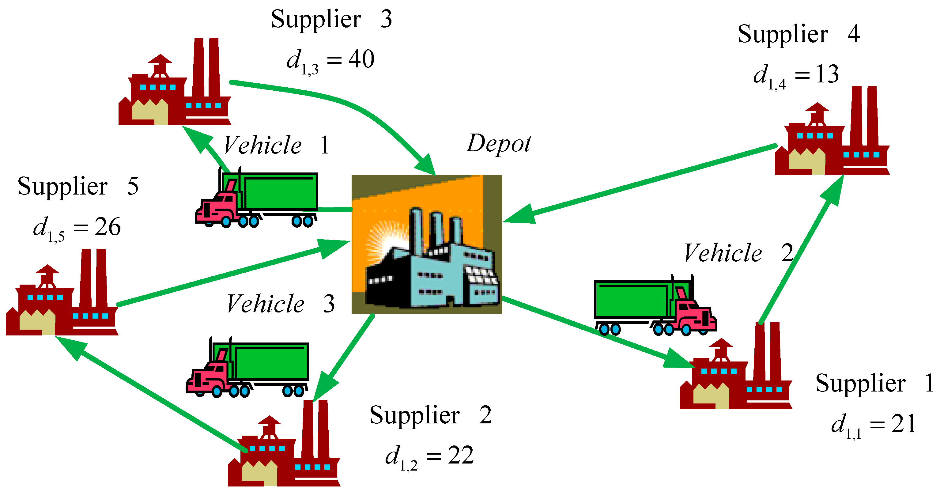
The MIP model is solved by LINGO 10, and the results are as follows. The transportation route and loading sizes of each vehicle in each period are shown in Table 8. Because of the travelling distance and the loading size limits of each vehicle, three vehicles are required in each period. For example, Vehicle 1 travels from the depot to Supplier 3 and ships 40 units of materials back to the depot in period 1. Vehicle 2 travels from the depot to Supplier 1 to pick up 21 units of materials, to Supplier 4 to pick up 13 units of materials, and then back to the depot. Vehicle 3 travels from the depot to Supplier 2 to pick up 22 units, to Supplier 5 to pick up 26 units, and then back to the depot. The vehicle routing in Period 1 is depicted in Figure 1.
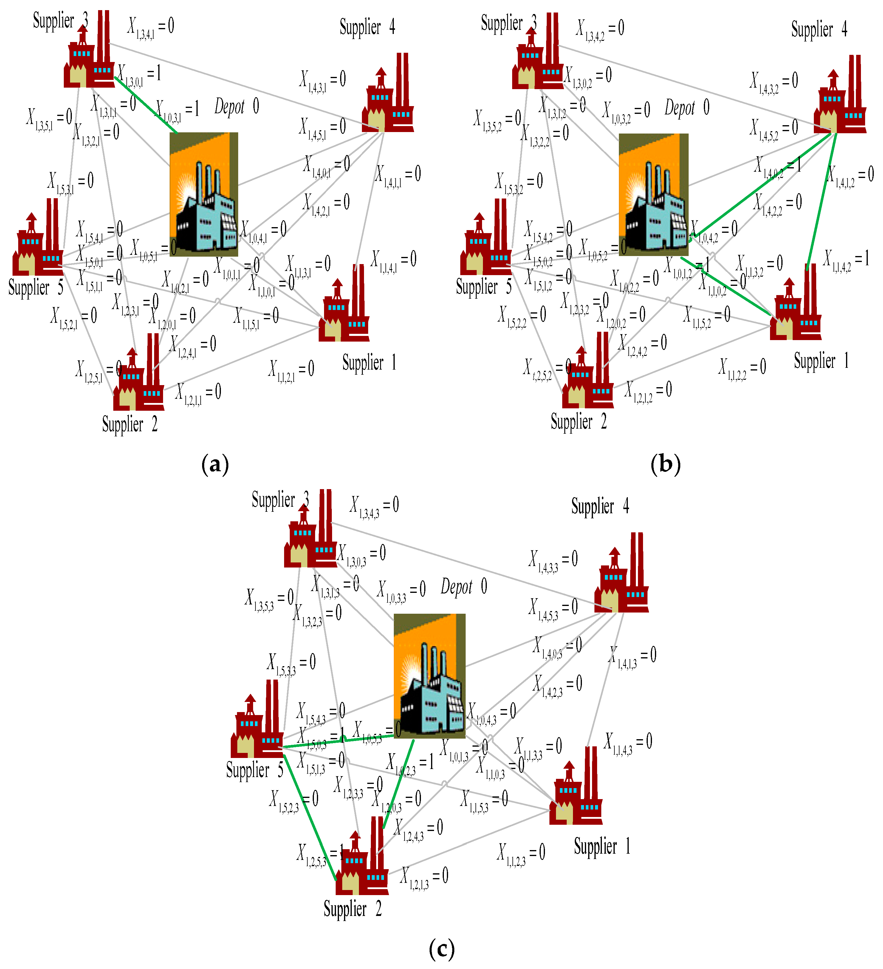
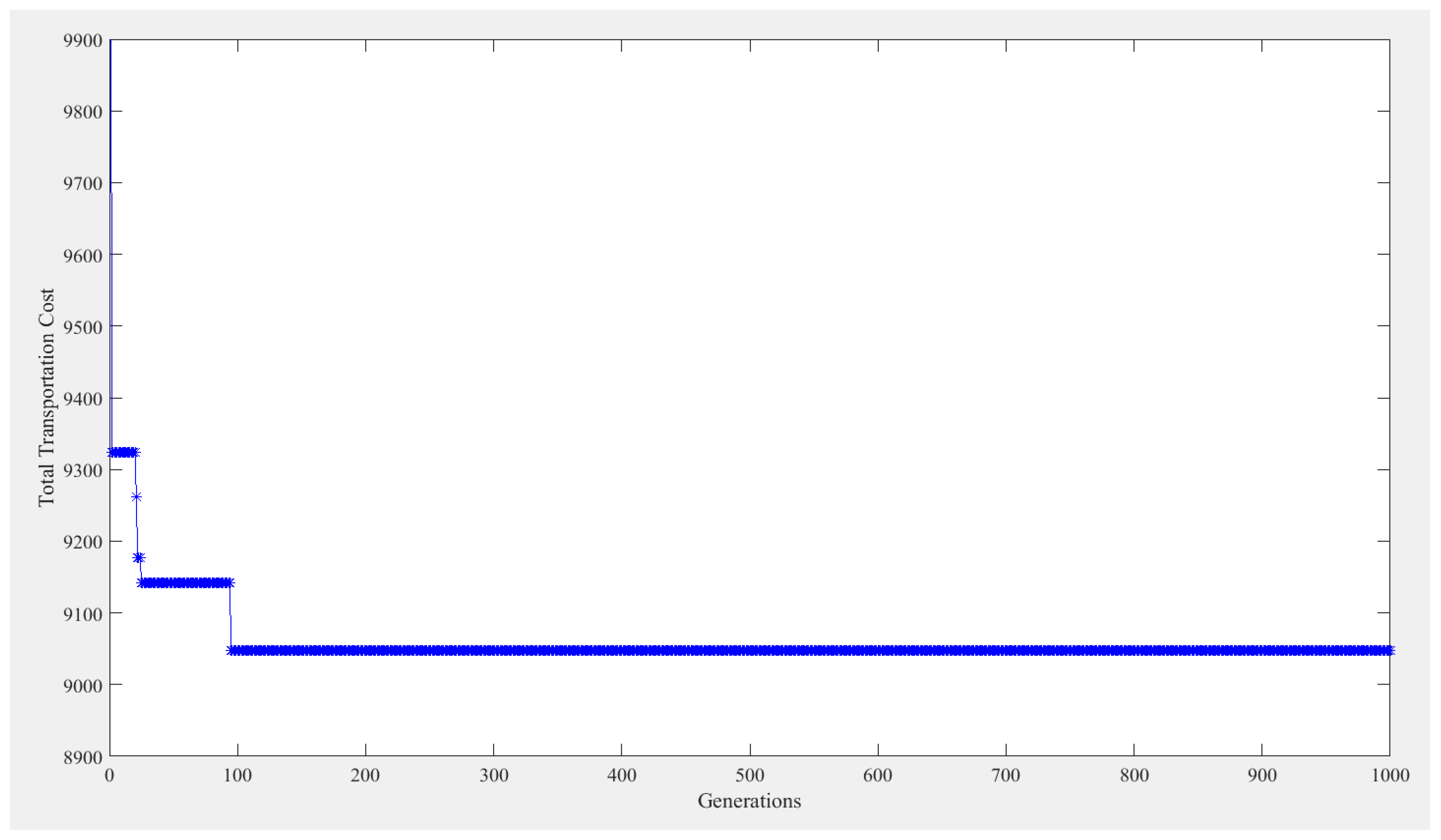
The GA model is next solved by MATLAB (2015). A two-cut-point crossover is adopted, and an inversion mutation operator is applied, to avoid a solution being trapped in a local optimum and to approach the global optimum. The initial population size is set as 50. The crossover rate is set as 0.85, that is, around 85% pairs of individuals are involved in the reproduction. The mutation rate is 0.15, indicating that each gene of a newly created solution is mutated, with a probability of 0.15. The algorithm is set to terminate at the 1000th generation. In case I, the best generation occurs at the 94th generation, as shown in Figure 2. The chromosome is coded as a string of i integer digits, and the i th gene is a binary number. When vehicle v travels from supplier node i to supplier node j in period t, the value for Xt,i,j,v equals one; otherwise, the value equals zero. In Period 1, the result from the GA shows X1,0,3,1 = 1 and X1,3,0,1 = 1 for Chromosome 1, X1,0,1,2 = 1, X1,1,4,2 = 1 and X1,4,0,2 = 1 for Chromosome 2, and X1,0,2,3 = 1, X1,2,5,3 = 1 and X1,5,0,3 = 1 for Chromosome 3. The routing can also be observed in Figure 3. For example, in Period 1, Vehicle 1 travels from the depot to supplier 3 (X1,0,3,1 = 1), and then back to the depot (X1,3,0,1 = 1).
The results of Case I, generated by the MIP model and by the GA model are the same, as shown in Table 9. The assigning cost is $4000, the travelling cost is $4888, the tardiness cost is $143, and the total transportation cost is $9031. The computational times using the MIP and the GA are 0.5 s and 105 s, respectively. Thus, the MIP is effective in this case study.
Case II
In Case II, there are nine suppliers and four vehicles, including one small vehicle, two medium vehicles and one large vehicle. Vehicle 1 is a small truck, Vehicles 2 and 3 are medium trucks, and Vehicle 4 is a large truck. The planning horizon contains seven periods. The demand information from nine suppliers is as shown in Table 10.
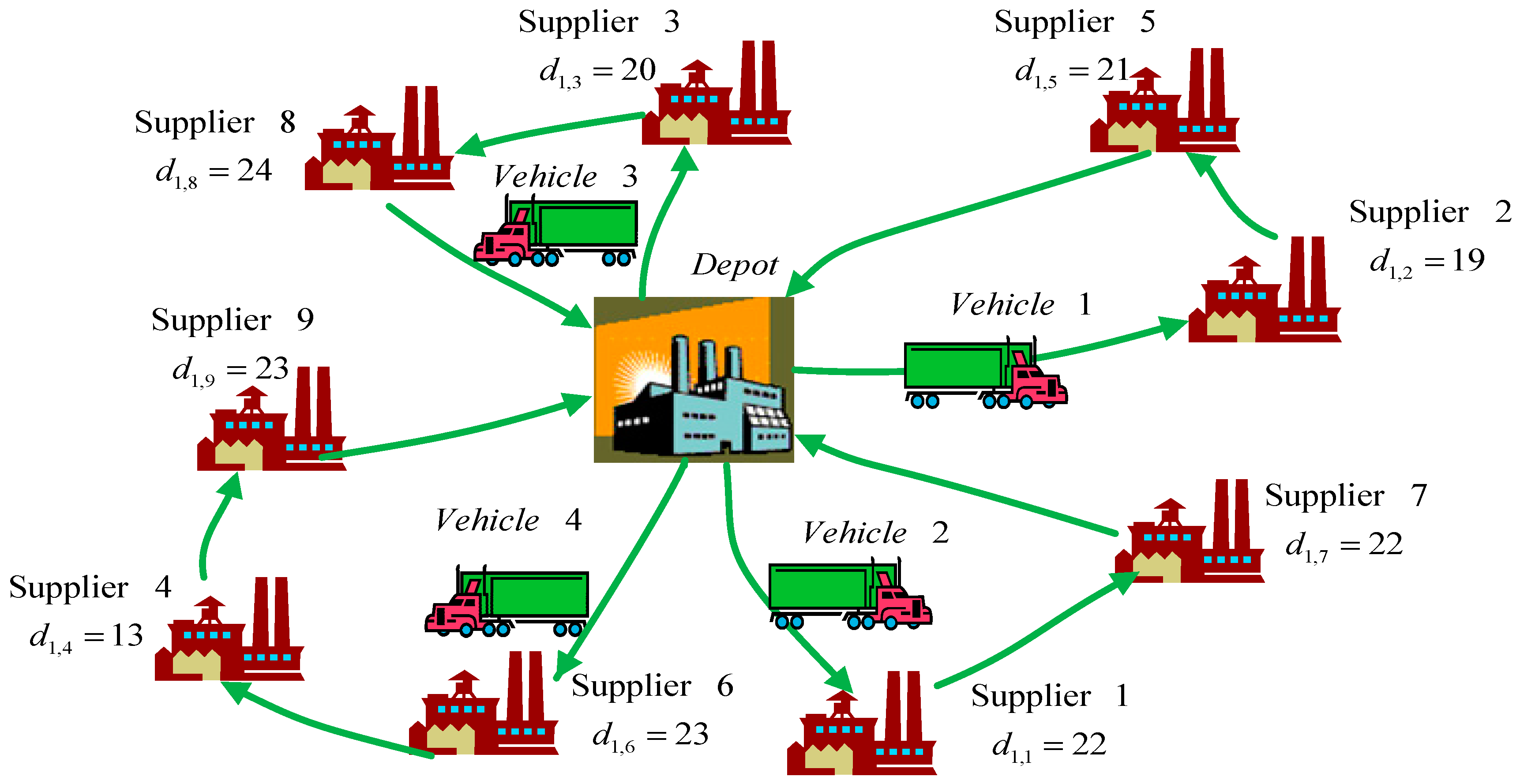
The transportation route and loading sizes of each vehicle in each period under the MIP are shown in Table 11. Three vehicles are required in each period. For example, Vehicle 1 travels from the depot to Supplier 2 and picks up 19 units of materials, to Supplier 5 and picks up 21 units of materials, and back to the depot in Period 1. Vehicle 2 travels from the depot to Supplier 1 to pick up 22 units of materials, to Supplier 7 to pick up 22 units of materials, and then back to the depot. The vehicle routing in Period 1 under the MIP is depicted in Figure 4.
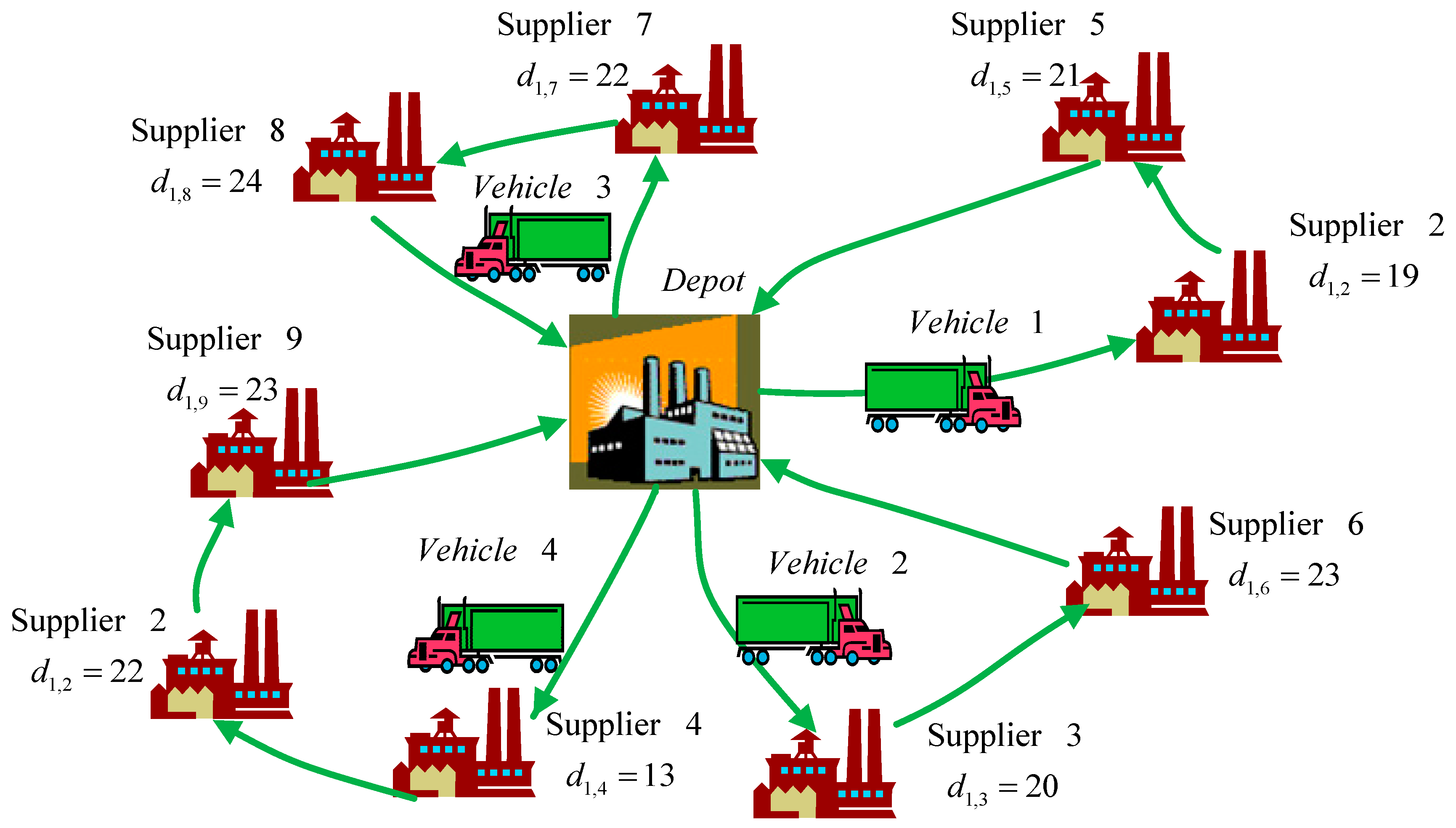
Table 12 shows the transportation route and loading sizes of each vehicle in each period under the GA. Four vehicles are required in each period. For example, Vehicle 1 travels from the depot to Supplier 2 and picks up 19 units of materials, to Supplier 5 and picks up 21 units of materials, and back to the depot in Period 1. Vehicle 2 travels from the depot to Supplier 3 to pick up 20 units of materials, to Supplier 6 to pick up 23 units of materials, and then back to the depot. Figure 5 depicts the vehicle routing in Period 1 under the GA.
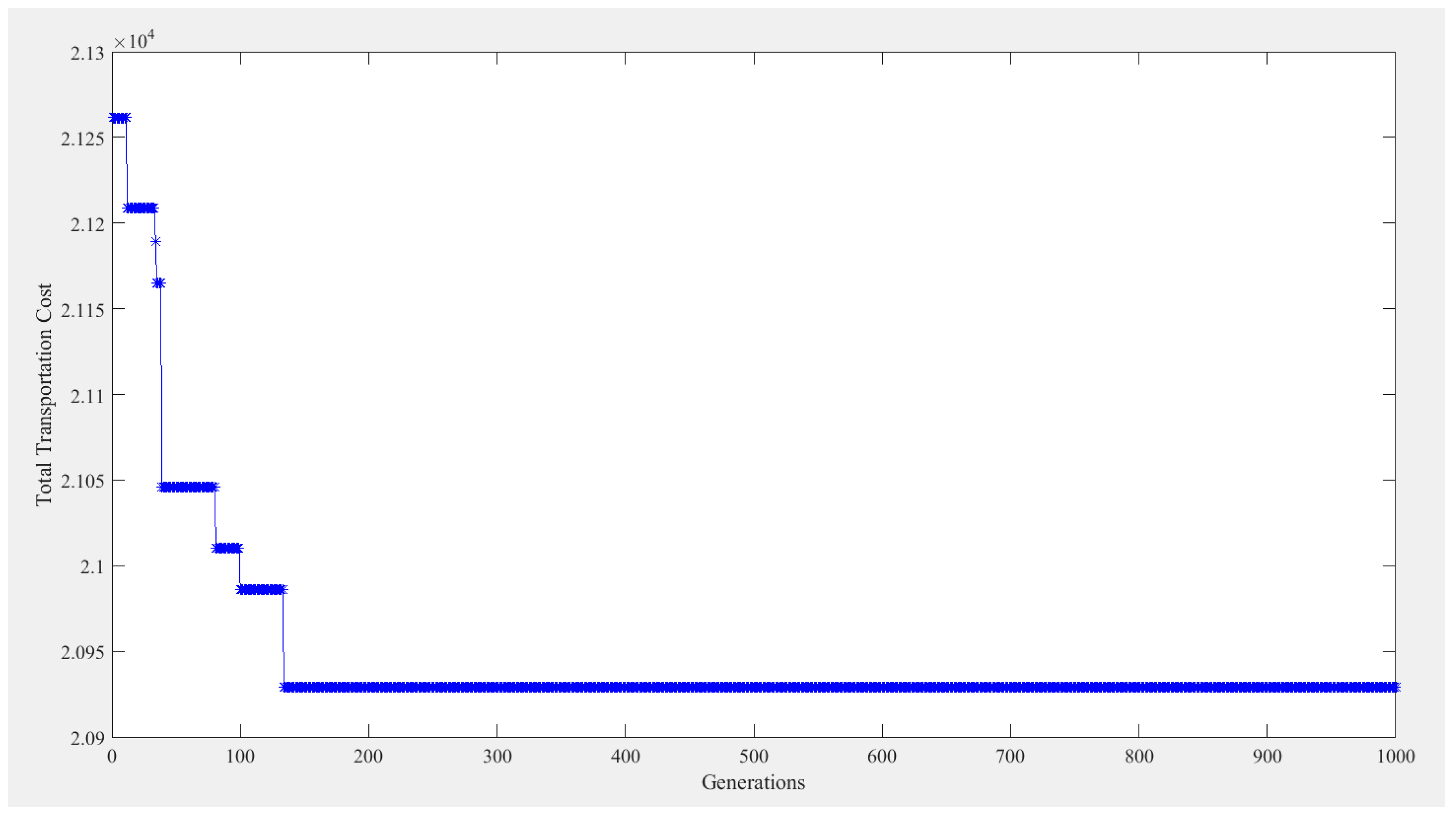
Table 13 shows that the results from the MIP and the GA. Under the MIP, the assigning cost is $8400, the travelling cost is $11,521.5, the tardiness cost is $193.6, and the total transportation cost is $20,115.1. Under the GA, the assigning cost, travelling cost, tardiness cost, and the total transportation cost are $8400, $12,013.1, $505.4, and $20,918.5, respectively. The total transportation cost under the GA is $803.4 higher than that under the MIP, with a difference of 3.99%. The computational time is 19 s under the MIP. Figure 6 shows the execution results from the GA. The size of the initial population is 100. The crossover rate and the mutation rate are 0.85 and 0.15, respectively. The algorithm is set to terminate at the 1000th generation. In the end, the computational time is 95 s, and the optimal solution is generated at the 133rd generation.
Case III
There are 15 factories in Case III. There are three kinds of vehicles, with one small vehicle, two medium vehicles, and two large vehicles. Vehicle 1 is a small truck, vehicle 2 and 3 are medium trucks, and vehicle 4 and 5 are large trucks. The planning horizon contains nine periods. The demand information from 12 suppliers is as shown in Table 14.
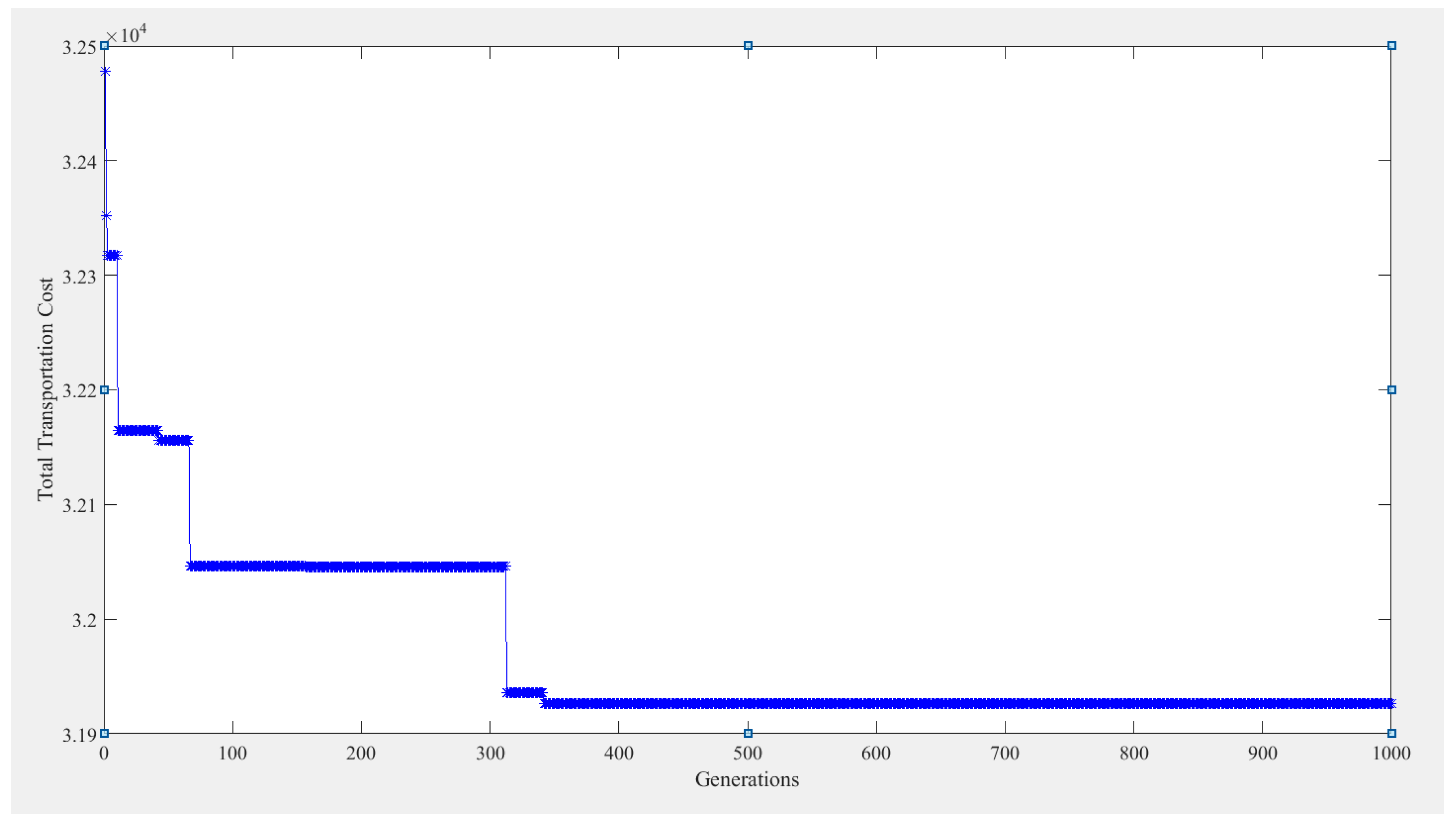
Because of the increase in the parameters and the decision variables, the problem becomes more complicated to be solved by the MIP. In fact, the problem in Case III is NP-hard. Therefore, only the GA is adopted to solve the problem. The results are shown in Table 15 and Table 16. Table 15 shows the transportation route and loading sizes of each vehicle in each period under the GA, and all five vehicles are required in each period. Table 16 shows that the relevant costs results from the GA. The assigning cost is $14,400, the travelling cost is $17,200, the tardiness cost is $332.6, and the total transportation cost is $31,952.6. Figure 7 depicts the vehicle routing in Period 1 under the GA. Figure 8 shows the execution results from the GA. The size of the initial population is 150, the crossover rate is 0.85, and the mutation rate is 0.15. The algorithm is set to terminate at the 1000th generation. The computational time is 203 s, and the optimal solution is generated at the 312nd generation.

5. Conclusions

Vehicle routing problem (VRP) has been studied abundantly to determine the optimal set of routes for a fleet of vehicles to travel so that certain objectives can be achieved, such as reducing the total cost for a firm. To the authors’ knowledge, this is the first instance of research that constructs a multiple vehicle routing problem (MVRP) model with a soft time window and heterogeneous vehicles. The contributions of this research are as follows. First, the MIP is used to construct a general formulation of the MVRP model. The model comprises the costs, including assigning cost, travelling cost, and tardiness cost for each planning period, and the goal aims to minimize the total transportation cost. Second, to tackle complex instances efficiently, a genetic algorithm (GA) model is proposed. Third, to examine the proposed MIP and GA models, two small-scale cases are studied, and both models can generate the optimal solutions. Fourth, a complicated case is used to examine the GA model. While the MIP model cannot solve the problem or it may require a very long time to perform the calculations if a case becomes too complicated, the proposed GA model can obtain near-optimal solutions in a short computational time. Therefore, the GA model can be effective in searching for near-optimal solutions. The proposed models, especially the GA model, can be valuable techniques for managers in real business settings. For example, based on the outcomes of the models, managers can determine the optimal or near optimal method for assigning the routings of multiple vehicles in each period, and for allocating loading sizes for each vehicle in each period, while aiming to minimize the total transportation cost.
In the future, a more comprehensive case for MVRP in manufacturing can be researched. Some assumptions are made in this research, such as fixed demand, fixed lead time, and one kind of product. A model that considers the probability demand, fuzzy lead time, fuzzy-demand joint replenishment, safety stock, and different priorities of orders can be constructed. In addition, the ordering cost for each purchase may be variable. Furthermore, a fuzzy multi-objective problem can be studied, and both a fuzzy multi-objective programming model and a GA model can be proposed to tackle the problem. Other metaheuristics techniques, such as artificial immune system, particle swarm optimization, ant colony system and revised aforementioned metaheuristics, may also be adopted. The methods can be compared and contrasted to examine which method is more appropriate for solving the MVRP.

Author Contributions

Conceptualization, H.-Y.K. and A.H.I.L.; Methodology, H.-Y.K. and A.H.I.L.; Software, H.-Y.K.; Validation, A.H.I.L.; Formal Analysis, A.H.I.L.; Investigation, H.-Y.K.; Resources, H.-Y.K. and A.H.I.L.; Writing-Original Draft Preparation, H.-Y.K. and A.H.I.L.; Writing-Review & Editing, A.H.I.L. and H.-Y.K.; Visualization, H.-Y.K.; Supervision, H.-Y.K. and A.H.I.L.; Project Administration, H.-Y.K. and A.H.I.L.; Funding Acquisition, H.-Y.K. and A.H.I.L.

Funding

This work was supported in part by the Ministry of Science and Technology in Taiwan under Grant MOST 105-2410-H-167-006-MY2 and MOST 104-2410-H-216-006-MY3.

Conflicts of Interest

The authors declare no conflict of interest.

Notations for the MIP

Indices:
i, jSupplier node (i = 0,1,2,…, I, j = 0,1,2,…, I, depot = 0, supplier = 1,2,3,…, I)
tPeriod
vNumber of vehicles
Sets:
I Set of suppliers i { 0 , 1 , 2 , , I }
T Set of periods t { 1 , 2 , 3 , , T }
V Set of vehicles v { 1 , 2 , 3 , , V }
Parameters:
d t , g Demand from supplier i in period t
τ v Fixed cost for assigning vehicle v
π i , j Travelling distance from supplier i to supplier j
w i , j Travelling time from supplier i to supplier j
u i Unload time at supplier i
l i Latest soft time to start the service at supplier i.
p i Tardiness cost per unit time charged by supplier i when a vehicle arrives after the latest soft time.
q v Maximum loading size for vehicle v
r v Maximum travelling distance for vehicle v
M Arbitrary large number
Decision variables:
X t , i , j , v Binary variable, 1 indicates that vehicle v travels from supplier i to supplier j in period t, and 0 indicates that no travel is incurred
L t , i , v Tardiness time of vehicle v when arriving supplier i in period t.
S t , i , v Service start time for supplier i served by vehicle v in period t.

References

  1. Baños, R.; Ortega, J.; Gil, C.; Márquez, A.L.; De Toro, F. A Hybrid Metaheuristic for Multi-objective Vehicle Routing Problems with Time Windows. Comput. Ind. Eng. 2013, 65, 286–296. [Google Scholar] [CrossRef]
  2. Zare-Reisabadi, E.; Mirmohammadi, S.H. Site Dependent Vehicle Routing Problem with Soft Time Window: Modeling and Solution Approach. Comput. Ind. Eng. 2015, 90, 177–185. [Google Scholar] [CrossRef]
  3. Adelzadeh, M.; Asl, V.M.; Koosha, M. A Mathematical Model and a Solving Procedure for Multi-depot Vehicle Routing Problem with Fuzzy Time Window and Heterogeneous Vehicle. Int. J. Adv. Manuf. Technol. 2014, 75, 793–802. [Google Scholar] [CrossRef]
  4. Dantzig, G.B.; Ramser, J.H. The Truck Dispatching Problem. Manag. Sci. 1959, 6, 80–91. [Google Scholar] [CrossRef]
  5. Abdoli, B.; MirHassani, S.A.; Hooshmand, F. Model and Algorithm for Bi-fuel Vehicle Routing Problem to Reduce GHG Emissions. Environ. Sci. Pollut. Res. 2017, 24, 21610–21624. [Google Scholar] [CrossRef] [PubMed]
  6. Toth, P.; Vigo, D. The Vehicle Routing Problem; Society for Industrial and Applied Mathematics: Philadelphia, PA, USA, 2002. [Google Scholar]
  7. Laporte, G. Fifty Years of Vehicle Routing. Transp. Sci. 2009, 43, 408–416. [Google Scholar] [CrossRef]
  8. Pillac, V.; Gendreau, M.; Gueret, C.; Medaglia, A.L. A Review of Dynamic Vehicle Routing Problems. Eur. J. Oper. Res. 2013, 225, 1–11. [Google Scholar] [CrossRef] [Green Version]
  9. Toth, P.; Vigo, D. Vehicle Routing: Problems, Methods, and Applications, 2nd ed.; Society for Industrial and Applied Mathematics: Philadelphia, PA, USA, 2014. [Google Scholar]
  10. Lee, Y.C.E.; Chan, C.K.; Langevin, A.; Lee, H.W.J. Integrated inventory-transportation model by synchronizing delivery and production cycles. Transp. Res. Part E Logist. Transp. Rev. 2016, 91, 68–89. [Google Scholar] [CrossRef]
  11. Ombuki, B.; Ross, B.J.; Hanshar, F. Multi-Objective Genetic Algorithms for Vehicle Routing Problem with Time Windows. Appl. Intell. 2006, 24, 17–30. [Google Scholar] [CrossRef] [Green Version]
  12. Michalewicz, Z. Genetic Algorithm + Data Structures = Evolution Programs; Springer: New York, NY, USA, 1996. [Google Scholar]
  13. Goldberg, D.E. Genetic Algorithms in Search, Optimization and Machine Learning; Addison-Wesley: Boston, MA, USA, 1989. [Google Scholar]
  14. Megala, N.; Jawahar, N. Genetic Algorithm and Hopfield Neural Network for a Dynamic Lot Sizing Problem. Int. J. Adv. Manuf. Technol. 2006, 27, 1178–1191. [Google Scholar] [CrossRef]
  15. Karthikeyan, P.; Baskar, S. Genetic algorithm with ensemble of immigrant strategies for multicast routing in Ad hoc networks. Soft Comput. 2015, 19, 489–498. [Google Scholar] [CrossRef]
  16. Kang, H.Y.; Pearn, W.L.; Chung, I.P.; Lee, A.H.I. An Enhanced Model for the Integrated Production and Transportation Problem in a Multiple Vehicles Environment. Soft Comput. 2016, 20, 1415–1435. [Google Scholar] [CrossRef]
  17. Lee, C.G.; Epelman, M.A.; White, C.C., III; Yavuz, A.B. A shortest path approach to the multiple-vehicle routing problem with split pick-ups. Transp. Res. Part B Methodol. 2006, 40, 265–284. [Google Scholar] [CrossRef] [Green Version]
  18. Duan, Z.; Sun, S.; Sun, S.; Li, W. Stochastic Time-dependent Vehicle Routing Problem: Mathematical Models and Ant Colony Algorithm. Adv. Mech. Eng. 2015, 7, 1–16. [Google Scholar] [CrossRef]
  19. Hooshmand Khaligh, F.; MirHassani, S.A. A Mathematical Model for Vehicle Routing Problem under Endogenous Uncertainty. Int. J. Prod. Res. 2016, 54, 579–590. [Google Scholar] [CrossRef]
  20. Liu, L.; Li, K.; Liu, Z. A Capacitated Vehicle Routing Problem with Order Available Time in E-commerce Industry. Eng. Optim. 2017, 49, 449–465. [Google Scholar] [CrossRef]
  21. Hernandez, F.; Gendreau, M.; Potvin, J.Y. Heuristics for Tactical Time Slot Management: A Periodic Vehicle Routing Problem View. Int. Trans. Oper. Res. 2017, 24, 1233–1252. [Google Scholar] [CrossRef]
  22. Khodabandeh, E.; Bai, L.; Heragu, S.S.; Evans, G.W.; Elrod, T.; Shirkness, M. Modelling and Solution of a Large-scale Vehicle Routing Problem at GE Appliances and Lighting. Int. J. Prod. Res. 2017, 55, 1100–1116. [Google Scholar] [CrossRef]
  23. Fisher, M.L.; Jaikumar, R. A Generalized Assignment Heuristic for Vehicle Routing. Networks 1981, 11, 109–124. [Google Scholar] [CrossRef]
  24. Mancini, S. A Combined Multistart Random Constructive Heuristic and Set Partitioning Based Formulation for the Vehicle Routing Problem with Time Dependent Travel Times. Comput. Oper. Res. 2017, 88, 290–296. [Google Scholar] [CrossRef]
  25. Yassen, E.T.; Ayob, M.; Nazri, M.Z.A.; Sabar, N.R. An Adaptive Hybrid Algorithm for Vehicle Routing Problems with Time Windows. Comput. Ind. Eng. 2017, 113, 382–391. [Google Scholar] [CrossRef]
  26. Soysal, M.; Çimen, M. A Simulation Based Restricted Dynamic Programming Approach for the Green Time Dependent Vehicle Routing Problem. Comput. Oper. Res. 2017, 88, 297–305. [Google Scholar] [CrossRef]
  27. Mousavi, S.M.; Vahdani, B. A robust approach to multiple vehicle location-routing problems with time windows for optimization of cross-docking under uncertainty. J. Intell. Fuzzy Syst. 2017, 32, 49–62. [Google Scholar] [CrossRef]
  28. Govindan, K.; Jafarian, A.; Khodaverdi, R.; Devika, K. Two-echelon multiple-vehicle location–routing problem with time windows for optimization of sustainable supply chain network of perishable food. Int. J. Prod. Econ. 2014, 152, 9–28. [Google Scholar] [CrossRef]
  29. Madankumar, S.; Rajendran, C. Mathematical Models for Green Vehicle Routing Problems with Pickup and Delivery: A Case of Semiconductor Supply Chain. Comput. Oper. Res. 2018, 89, 183–192. [Google Scholar] [CrossRef]
  30. Dalmeijer, K.; Spliet, R. A Branch-and-cut Algorithm for the Time Window Assignment Vehicle Routing Problem. Comput. Oper. Res. 2018, 89, 140–152. [Google Scholar] [CrossRef]
  31. Xu, H.; Pu, P.; Duan, F. Dynamic Vehicle Routing Problems with Enhanced Ant Colony Optimization. Discrete Dyn. Nat. Soc. 2018. [Google Scholar] [CrossRef]
  32. Baker, B.M.; Ayechew, M.A. A Genetic Algorithm for the Vehicle Routing Problem. Comput. Oper. Res. 2003, 30, 787–800. [Google Scholar] [CrossRef]
  33. Alvarenga, G.B.; Mateus, G.R.; de Tomi, G. A Genetic and Set Partitioning Two-phase Approach for the Vehicle Routing Problem with Time Windows. Comput. Oper. Res. 2007, 34, 1561–1584. [Google Scholar] [CrossRef]
  34. Vidal, T.; Crainic, T.G.; Gendreau, M.; Lahrichi, N.; Rei, W. A Hybrid Genetic Algorithm for Multidepot and Periodic Vehicle Routing Problems. Oper. Res. 2012, 60, 611–624. [Google Scholar] [CrossRef]
  35. Vidal, T.; Crainic, T.G.; Gendreau, M.; Prins, C. A Hybrid Genetic Algorithm with Adaptive Diversity Management for a Large Class of Vehicle Routing Problems with Time-windows. Comput. Oper. Res. 2013, 40, 475–489. [Google Scholar] [CrossRef]
  36. Xiao, Y.; Konak, A. A Genetic Algorithm with Exact Dynamic Programming for the Green Vehicle Routing & Scheduling Problem. J. Clean Prod. 2017, 167, 1450–1463. [Google Scholar]
  37. Lee, A.H.I.; Kang, H.Y.; Lai, C.M.; Hong, W.Y. An Integrated Model for Lot Sizing with Supplier Selection and Quantity Discounts. Appl. Math. Model. 2013, 37, 4733–4746. [Google Scholar] [CrossRef]
  38. Lu, H.; Liu, J.; Niu, R.; Zhu, Z. Fitness Distance Analysis for Parallel Genetic Algorithm in the Test Task Scheduling Problem. Soft Comput. 2014, 18, 2385–2396. [Google Scholar] [CrossRef]
  39. Poon, P.W.; Carter, J.N. Genetic Algorithm Crossover Operators for Ordering Applications. Comput. Oper. Res. 1995, 22, 135–147. [Google Scholar] [CrossRef]
  40. Boese, K.D.; Kahng, A.B. Best-so-far vs. Where-you-are: Implications for Optimal Finite-time Annealing. Syst. Control. Lett. 1994, 22, 71–78. [Google Scholar] [CrossRef]
  41. LINGO System Inc. LINGO User’s Manual, version 10; LINGO System Inc.: Chicago, IL, USA, 2006. [Google Scholar]
  42. The MathWorks, Inc. MATLAB User’s Manual, version 8.6; The MathWorks, Inc.: Natick, MA, USA, 2015. [Google Scholar]
Figure 1. Vehicle routing in Period 1 under the MIP for Case I.
Symmetry 10 00650 g001
Figure 2. Results from the genetic algorithm (GA) using MATLAB for Case I.
Symmetry 10 00650 g002
Figure 3. Vehicle routing in Period 1. (a) Vehicle v = 1 in Period 1; (b) Vehicle v = 2 in Period 1; (c) Vehicle v = 3 in Period 1.
Symmetry 10 00650 g003
Figure 4. Vehicle routing in Period 1 under the MIP for Case II.
Symmetry 10 00650 g004
Figure 5. Vehicle routing in period 1 under the GA for Case II.
Symmetry 10 00650 g005
Figure 6. Results from the GA using MATLAB for Case II.
Symmetry 10 00650 g006
Figure 7. Vehicle routing in Period 1 under the GA for Case III.
Symmetry 10 00650 g007
Figure 8. Results from the GA using MATLAB for Case III.
Symmetry 10 00650 g008
Table 1. Vehicle assignment and travelling cost.
Vehicle12345
Vehicle typeSMMLL
Assigning cost ( τ v )$200$300$300$400$400
Unit travelling cost ( ρ v )$0.9$1$1$1.1$1.1
Table 2. Limits of vehicles.
Vehicle12345
Loading ( h v ) 4050506060
Travelling distance ( l v ) 300550550660660
Unit of measure for h v : unit; l v : km.
Table 3. Data of suppliers.
Supplieri = 123456789101112
ui11101221101315128161311
pi$1.1$2.1$3.2$2.2$2.3$3$5.2$4.4$2.6$3.7$2.5$1.4
li120260310160295340358415320340375455
Unit of measure for ui: min; pi: $/min; li: min.
Table 4. Travelling distance matrix among suppliers.
πijj = 0123456789101112
i = 0015010012021010013515012785175120115
1150016031012019514015821522740175255
21001600150145655525024519014740173
31203101500285952002561788226512435
421012014528502057027031029032169309
51001956595205011527023516020761125
61351405520070115026027522510080225
71501582502562702702600111195215283254
8127215245178310235275111080305265143
9852271908229016022519580029019855
1017540147265322071002153052900180289
111201754012416961802832651981800168
1211525517335309125225254143552891680
Unit of measure: km.
Table 5. Travelling time matrix among suppliers.
wijj = 0123456789101112
i = 00 90 60 72 126 60 81 90 76 51 105 72 69
190 0 96 186 72 117 84 95 129 136 24 105 153
260 96 0 90 87 39 33 150 147 114 88 24 104
372 186 90 0 171 57 120 154 107 49 159 74 21
4126 72 87 171 0 123 42 162 186 174 19 101 185
560 117 39 57 123 0 69 162 141 96 124 37 75
681 84 33 120 42 69 0 156 165 135 60 48 135
790 95 150 154 162 162 156 0 67 117 129 170 152
876 129 147 107 186 141 165 67 0 48 183 159 86
951 136 114 49 174 96 135 117 48 0 174 119 33
10105 24 88 159 19 124 60 129 183 174 0 108 173
1172 105 24 74 101 37 48 170 159 119 108 0 101
1269 153 104 21 185 75 135 152 86 33 173 101 0
Unit of measure: min.
Table 6. Problem configuration.
CasePeriod NumberSupplier NumberVehicle NumberTransportation NetworkVariable Number for MIPConstraint Number for MIP
I5536 × 69311171
II79410 × 1039033977
III912513 × 1397589919
Table 7. Demand from suppliers for Case I.
Supplier12345
Period
12122401326
22624232430
3282031917
4302624826
52212322823
Table 8. Vehicle routing and loading sizes under the MIP for Case I.
PeriodVehicleVehicle Routing and Loading Size
11Depot → Supplier 3 (40) → Depot
2Depot → Supplier 1 (21) → Supplier 4 (13) → Depot
3Depot → Supplier 2 (22) → Supplier 5 (26) → Depot
21Depot → Supplier 5 (30) → Depot
2Depot → Supplier 3 (23) → Supplier 2 (24) → Depot
3Depot → Supplier 1 (26) → Supplier 4 (24) → Depot
31Depot → Supplier 3 (31) → Depot
2Depot → Supplier 2 (20) → Supplier 5 (17) → Depot
3Depot → Supplier 1 (28) → Supplier 4 (9) → Depot
41Depot → Supplier 2 (26) → Depot
2Depot → Supplier 3 (24) → Supplier 5 (26) → Depot
3Depot → Supplier 1 (30) → Supplier 4 (8) → Depot
51Depot → Supplier 3 (32) → Depot
2Depot → Supplier 2 (12) → Supplier 5 (23) → Depot
3Depot → Supplier 1 (22) → Supplier 4 (28) → Depot
Table 9. Relevant costs for Case I.
CostAssigning CostTravelling CostTardiness CostTotal Transportation Cost
MIP400048881439031
GA400048881439031
Error = 0.00%
Table 10. Demand from suppliers for Case II.
Supplier123456789
Period
1221920132123222423
2262430172516242120
324261926172820921
4301524112430162418
5222025282322132119
621171921232116928
7221330281322122124
Table 11. Vehicle routing and loading sizes under the MIP for Case II.
PeriodVehicleVehicle Routing and Loading Size
11Depot → Supplier 2 (19) → Supplier 5 (21) → Depot
2Depot → Supplier 1 (22) → Supplier 7 (22) → Depot
3Depot → Supplier 3 (20) → Supplier 8 (24) → Depot
4Depot → Supplier 6 (23) →Supplier 4 (13) →Supplier 9 (23) → Depot
21Depot → Supplier 3 (30) → Supplier 9 (10) → Depot
2Depot → Supplier 1 (26) → Supplier 7 (24) → Depot
3Depot → Supplier 5 (25) → Supplier 8 (21) → Depot
4Depot → Supplier 4 (17) → Supplier 6 (16) → Supplier 2 (24) → Depot
31Depot → Supplier 3 (19) → Supplier 9 (21) → Depot
2Depot → Supplier 1 (24) → Supplier 4 (26) → Depot
3Depot → Supplier 2 (16) → Supplier 6 (28) → Depot
4Depot → Supplier 5 (17) → Supplier 8 (19) → Supplier 7 (20) → Depot
41Depot → Supplier 2 (15) → Supplier 5 (24) → Depot
2Depot → Supplier 1 (30) → Supplier 7 (16) → Depot
3Depot → Supplier 3 (24) → Supplier 8 (24) → Depot
4Depot → Supplier 6 (30) → Supplier 4 (11) → Supplier 9 (18) → Depot
51Depot → Supplier 8 (21) → Supplier 9 (19) → Depot
2Depot → Supplier 3 (25) → Supplier 5 (23) → Depot
3Depot → Supplier 4 (28) → Supplier 6 (22) → Depot
4Depot → Supplier 2 (20) → Supplier 1 (22) → Supplier 7 (13) → Depot
61Depot → Supplier 2 (17) → Supplier 6 (21)→ Depot
2Depot → Supplier 1 (21) → Supplier 4 (21) → Depot
3Depot → Supplier 3 (19) → Supplier 5 (23)→ Depot
4Depot → Supplier 7 (16) → Supplier 8 (9) → Supplier 9 (28) → Depot
71Depot → Supplier 3 (30) → Depot
2Depot → Supplier 1 (22) → Supplier 4 (28) → Depot
3Depot → Supplier 5 (13) → Supplier 2 (13) → Supplier 6 (22) → Depot
4Depot → Supplier 7 (22) → Supplier 8 (21) → Supplier 9 (12) → Depot
Table 12. Vehicle routing and loading sizes under the GA for Case II.
PeriodVehicleVehicle Routing and Loading Size
11Depot → Supplier 2 (19) → Supplier 5 (21)→ Depot
2Depot → Supplier 3 (20) → Supplier 6 (23) → Depot
3Depot → Supplier 7 (22) → Supplier 8 (24)→ Depot
4Depot → Supplier 4 (13) → Supplier 1 (22) → Supplier 9 (23) → Depot
21Depot → Supplier 3 (30) → Supplier 9 (10)→ Depot
2Depot → Supplier 1 (26) → Supplier 7 (24) → Depot
3Depot → Supplier 5 (25) → Supplier 8 (21) → Depot
4Depot → Supplier 4 (17) → Supplier 2 (24) → Supplier 6 (16) → Depot
31Depot → Supplier 3 (19) → Supplier 9 (21) → Depot
2Depot → Supplier 1 (24) → Supplier 4 (26) → Depot
3Depot → Supplier 2 (16) → Supplier 6 (28) → Depot
4Depot → Supplier 5 (17) → Supplier 8 (19) → Supplier 7 (20) → Depot
41Depot → Supplier 2 (15) → Supplier 5 (24) → Depot
2Depot → Supplier 3 (24) → Supplier 8 (24) → Depot
3Depot → Supplier 6 (30) → Supplier 7 (16) → Depot
4Depot → Supplier 4 (11) → Supplier 1 (30) → Supplier 9 (18) → Depot
51Depot → Supplier 8 (21) → Supplier 9 (19) → Depot
2Depot → Supplier 1 (22) → Supplier 4 (28) → Depot
3Depot → Supplier 3 (25) → Supplier 5 (23) → Depot
4Depot → Supplier 6 (22) → Supplier 2 (12) → Supplier 7 (13) → Depot
61Depot → Supplier 2 (17) → Supplier 6 (21) → Depot
2Depot → Supplier 1 (21) → Supplier 4 (21) → Depot
3Depot → Supplier 3 (19) → Supplier 5 (23) → Depot
4Depot → Supplier 7 (16) → Supplier 8 (9) →Supplier 9 (28) → Depot
71Depot → Supplier 8 (21) → Supplier 9 (12) → Depot
2Depot → Supplier 3 (30) → Supplier 5 (13) → Depot
3Depot → Supplier 4 (28) → Supplier 6 (22) → Depot
4Depot → Supplier 2 (13) → Supplier 1 (22) → Supplier 7 (22) → Depot
Table 13. Relevant costs for Case II.
CostAssigning CostTravelling CostTardiness CostTotal Transportation Cost
MIP840011,521.5193.620,115.1
GA840012,013.1505.420,918.5
Error = 3.99%
Table 14. Demand from suppliers for Case III.
Supplier123456789101112
Period
1221920132123222413262424
2261420172526242120231219
32416926172820931222524
4301612112430162418152123
5221215282322132525232217
621171921232116928111816
7221330281322122120222711
821171921232116931211816
9221320281322121129222711
Table 15. Vehicle routing and loading sizes under the GA for Case III.
PeriodVehicleVehicle Routing and Loading Size
11Depot → Supplier 2 (19) → Supplier 5 (21) → Depot
2Depot → Supplier 6 (23) → Supplier 11 (24) → Depot
3Depot → Supplier 7 (22) → Supplier 8 (24) → Depot
4Depot → Supplier 10 (26) → Supplier 4 (13) → Supplier 3 (20) → Depot
5Depot → Supplier 1 (22) → Supplier 12 (24) → Supplier 9 (13) → Depot
21Depot → Supplier 3 (20) → Supplier 12 (19) → Depot
2Depot → Supplier 8 (21) → Supplier 9 (20) → Depot
3Depot → Supplier 1 (26) → Supplier 7 (24) → Depot
4Depot → Supplier 4 (17) → Supplier 6 (26) → Supplier 2 (14) → Depot
5Depot → Supplier 5 (25) → Supplier 11 (12) → Supplier 10 (23) → Depot
31Depot → Supplier 3 (9) → Supplier 9 (31) → Depot
2Depot → Supplier 1 (24) → Supplier 4 (26) → Depot
3Depot → Supplier 7 (20) → Supplier 12 (24) → Depot
4Depot → Supplier 2 (16) → Supplier 11 (25) → Supplier 5 (17) → Depot
5Depot → Supplier 6 (28) → Supplier 10 (22) → Supplier 8 (9) → Depot
41Depot → Supplier 2 (16) → Supplier 11 (21) → Depot
2Depot → Supplier 1 (30) → Supplier 10 (15) → Depot
3Depot → Supplier 4 (11) → Supplier 6 (30) → Depot
4Depot → Supplier 5 (24) → Supplier 3 (12) → Supplier 12 (23) → Depot
5Depot → Supplier 9 (18) → Supplier 8 (24) → Supplier 7 (16) → Depot
51Depot → Supplier 3 (15) → Supplier 12 (17) → Depot
2Depot → Supplier 8 (25) → Supplier 9 (25) → Depot
3Depot → Supplier 4 (28) → Supplier 6 (22) → Depot
4Depot → Supplier 2 (12) → Supplier 11 (22) → Supplier 5 (23) → Depot
5Depot → Supplier 10 (23) → Supplier 1 (22) → Supplier 7 (13) → Depot
61Depot → Supplier 2 (17) → Supplier 5 (23) → Depot
2Depot → Supplier 3 (19) → Supplier 12 (16) → Depot
3Depot → Supplier 1 (21) → Supplier 10 (11) → Depot
4Depot → Supplier 4 (21) → Supplier 6 (21) → Supplier 11 (18) → Depot
5Depot → Supplier 7 (16) → Supplier 8 (9) → Supplier 9 (28) → Depot
71Depot → Supplier 8 (11) → Supplier 9 (20) → Depot
2Depot → Supplier 3 (30) → Supplier 12 (11) → Depot
3Depot → Supplier 4 (28) → Supplier 6 (22) → Depot
4Depot → Supplier 10 (22) → Supplier 1 (22) → Supplier 7 (12) → Depot
5Depot → Supplier 2 (13) → Supplier 11 (27) → Supplier 5 (13) → Depot
81Depot → Supplier 2 (17) → Supplier 5 (23) → Depot
2Depot → Supplier 3 (19) → Supplier 12 (16) → Depot
3Depot → Supplier 8 (9) → Supplier 9 (31) → Depot
4Depot → Supplier 4 (21) → Supplier 6 (21) → Supplier 11 (18) → Depot
5Depot → Supplier 10 (21) → Supplier 1 (21) → Supplier 7 (16)→ Depot
91Depot → Supplier 3 (20) → Supplier 12 (11) → Depot
2Depot → Supplier 8 (21) → Supplier 9 (29) → Depot
3Depot → Supplier 4 (28) → Supplier 6 (22) → Depot
4Depot → Supplier 2 (13) → Supplier 11 (27) → Supplier 5 (13) → Depot
5Depot → Supplier 10 (22) → Supplier 1 (22) → Supplier 7 (12) → Depot
Table 16. Relevant costs for case III.
CostAssigning CostTravelling CostTardiness CostTotal Transportation Cost
GA14,40017,220332.631,952.6