Article

Design of a New Variable Shewhart Control Chart Using Multiple Dependent State Repetitive Sampling

1
Department of Statistics, Faculty of Science, King Abdulaziz University, Jeddah 21551, Saudi Arabia
2
Department of Statistics, Jhang Campus, University of Veterinary and Animal Sciences, Lahore 54000, Pakistan
3
Department of Industrial and Management Engineering, Pohang University of Science and Technology, Pohang 37673, Korea
*
Author to whom correspondence should be addressed.
Symmetry 2018, 10(11), 641; https://doi.org/10.3390/sym10110641
Submission received: 24 October 2018 / Revised: 12 November 2018 / Accepted: 14 November 2018 / Published: 15 November 2018

Abstract

:
In this paper, a new variable control chart is proposed using multiple dependent-state repetitive sampling by assuming that the data follows a normal distribution having a symmetry property. Its efficiency will be evaluated in terms of in-control and out-of-control average run lengths. The results showed that the proposed chart is better than the existing variable control chart to detect an early shift in the process. An industrial example is given to illustrate the proposed chart in the industry.

1. Introduction

Control charts are powerful, effective and important tools which are frequently used to detect unusual variation in the manufacturing process. This tool timely indicates the shift in the process due to unusual variation in the process and help engineers a corrective action. The main objective of control charts is to monitor the process and determine whether it is maintained in a stable state, which can be done by plotting statistics computed from a random sample from the process. The Shewhart control chart is very simple and popularly used for monitoring processes in the industry. These control charts are effective in detecting a large shift in the process but insensitive to detecting a small shift in the process. The Shewhart [1] X-bar control chart is very common to detect a shift in the mean of the process [2]. As suggested by Reference [3], the X-bar control chart is simple to apply when the quality of interest follows the normal distribution. Control charts have two control limits called upper control limit (UCL) and lower control limit (LCL). The process is said to be in control if a plotted statistic is between LCL and UCL. A process is said to be out-of-control if a plotted statistic beyond LCL or UCL and or the process may be considered out of control even if all points are within the control limits utilizing nine or more points in a row that are on the same side of the mean. Several authors designed variable control charts: for example, Reference [4] worked on the X-bar chart with variable sample size. Reference [5] Studies run length properties of the X-bar chart. Reference [6] proposed a EWMA chart for mean and variance. Reference [7] proposed an X-bar chart using double and triple sampling. Reference [8] applied the X-bar chart in the semiconductor industry. Reference [9] designed a multi-objective economic X-bar chart under Taguchi loss function and Reference [10] designed an economic X-bar chart using Taguchi loss function.
There are many sampling schemes including, for example, single sampling [5], double sampling, triple sampling [7,11], repetitive sampling [12] and multiple dependent-state sampling [13], which have been widely used in the design of control charts. Among all these sampling schemes, the control chart using single sampling is common as it is simple and easy to apply in the industry. The control charts using single sampling make a decision about the state of the process by plotting statistics computed from the single sample. However, a control chart using single sampling provides larger values of average run length (ARL) when the process is out-of-control. The late indication in the shifted process causes non-confirming items. The efficiency of control charts to detect a shift in the process can be improved using other sampling schemes [14]. More details about the control chart can be seen in References [15,16].
The control charts using a repetitive sampling scheme and multiple dependent state sampling are more efficient than control charts using a single sampling scheme [17,18]. Reference [19] introduced multiple dependent state repetitive (MDSR) sampling in the area of the acceptance sampling plan for lot disposition. They showed that MDSR sampling is more efficient in reducing sample size of the inspection lot as compared to repetitive and multiple dependent-state sampling. Reference [12] introduced the repetitive sampling in the area of the control chart which allows to repeat the sampling process if the plotting statistic lies in the in-decision state. Aslam et al. [13] introduced multiple dependent state (MDS) sampling in the area of control charts, which utilizes the previous subgroup information if the decision cannot be made based on the first sample. The MDSR sampling utilizes the previous subgroup information as well as repetitive process if the plotting statistic is in the in-decision state and the specified previous subgroups are not in the in-control state. By exploring the literature and to the best of the author’s knowledge, there is no work on variable control charts using MDSR sampling. In this paper, we will introduce the MDSR sampling scheme in the area of variable control charts. We will present the structure of the X-bar control chart using MDSR sampling. It is expected that the proposed X-bar chart will perform better than an existing control chart in terms of ARL. A simulation study and real example are given to illustrate the proposed control chart. In Section 2, the design of the proposed chart is given. The advantages of the proposed chart are given in Section 3. The industrial application is given in Section 4 and concluding remarks are given in the last section.

2. Design of Proposed Chart

Suppose that the quality of interest X follows the normal distribution with mean m and variance σ 2 . Let X ¯ = i = 1 n X i / n be the average of the random sample, where X i is the i-th measurement in a sample of size n. We proposed the following X ¯ control chart by utilizing multiple dependent-state repetitive sampling.
Step-1: A random sample of size n is selected from the production process and X ¯ = i = 1 n X i / n is computed from each subgroup.
Step-2 (Decision State): The process is said to be in control if LCL 2 X ¯ UCL 2 . The process is said to be out-of-control if X ¯ U C L 1 or X ¯ L C L 1 . Otherwise, go to Step-3. Here, L C L 1 , L C L 2 , U C L 1 and U C L 2 are control limits to be determined later.
Step-3 (Indecision State): If U C L 2 X ¯ U C L 1 or L C L 1 X ¯ L C L 2 . The process is declared in control if i proceeding subgroups have been declared as in control. Otherwise, repeat Step-1.
The proposed control chart has four control limits L C L 1 , L C L 2 , U C L 1 and U C L 2 and two control chart coefficients k 1 and k 2 to be determined. The proposed control chart is more generalized than X ¯ control chart. Several X ¯ charts are special cases for the proposed chart. For example, when k 1 = k 2 it becomes Shewhart X ¯ chart. The proposed chart reduces to X ¯ chart using MDS sampling when the probability of repetition is zero or repetition is not allowed. The proposed chart reduces to X ¯ chart using repetitive sampling when i = 0. The four control limits of the proposed X ¯ chart is given as:
U C L 1 = m + k 1 σ / n
L C L 1 = m k 1 σ / n
U C L 2 = m + k 2 σ / n
L C L 2 = m k 2 σ / n
Here, control constants k 1 and k 2 will be determined by considering the target in-control average run length.

2.1. Measures for in-Control Process

The probability of declaring as in-control at μ = m , say P in , 1 0 , for a single sample, is given by
P i n , 1 0 = P ( L C L 2 X ¯ U C L 2 ) +   { P ( L C L 1 < X ¯ < L C L 2 ) + P ( U C L 2 < X ¯ < U C L 1 ) } { P ( L C L 2 X ¯ U C L 2 ) } i
When plotting statistics in an indecision state, the process is repeated as stated in Step-3 of the proposed control chart. Let P rep 0 denote the probability for this area. Then, it is given as follows
P r e p 0 = { P ( L C L 1 < X ¯ < L C L 2 ) + P ( U C L 2 < X ¯ < U C L 1 ) } ( 1 [ P { L C L 2 X ¯ U C L 2 } ] i )
The process is said to be out-of-control if the plotting statistic X ¯ lies beyond U C L 1 or L C L 1 . Let P out , 1 0 denote the probability that the process is declared to be out-of-control. Then, it is given by
P out , 1 0 = P ( X ¯ U C L 1 ) + P ( X ¯ L C L 1 )
The probability in (5) is obtained by
P in , 1 0 = ( 2 Φ ( k 2 ) 1 ) + 2 { Φ ( k 1 ) Φ ( k 2 ) } { 2 Φ ( k 2 ) 1 } i
The probability of repetition in (6) is given as
P rep 0 = 2 { Φ ( k 1 ) Φ ( k 2 ) } ( 1 [ 2 Φ ( k 2 ) 1 ] i )
Therefore, the probability that the process is declared as in-control for the proposed X ¯ chart using MDSR sampling is given as follows
P in 0 = P i n , 1 0 1 P rep 0 = ( 2 Φ ( k 2 ) 1 ) + 2 { Φ ( k 1 ) Φ ( k 2 ) } { 2 Φ ( k 2 ) 1 } i 1 { 2 { Φ ( k 1 ) Φ ( k 2 ) } ( 1 [ 2 Φ ( k 2 ) 1 ] i ) }
The ARL when the process is in-control is calculated as follows
A R L 0   =   1 1 ( ( 2 Φ ( k 2 ) 1 ) + 2 { Φ ( k 1 ) Φ ( k 2 ) } { 2 Φ ( k 2 ) 1 } i )

2.2. Measures for Out-of-Control Process

Assume that due to some factors, the process has shifted from μ to a new mean μ 1 = m + c σ , where c is a constant indicating a shift in the process. The necessary measures for the shifted process are derived as follows.
Let P in , 1 1 denote the probability that the process is declared as in-control at μ 1 . Then, it is given as
P in , 1 1 = P ( L C L 2 X ¯ U C L 2 | μ 1 ) +   { P ( L C L 1 < X ¯ < L C L 2 | μ 1 ) + P ( U C L 2 < X ¯ < U C L 1 | μ 1 ) } { P ( L C L 2 X ¯ U C L 2 | μ 1 ) } i
The probability of repeated sampling, say P rep 1 at μ 1 is given as
P rep 1 = { P ( L C L 1 < X ¯ < L C L 2 | μ 1 ) + P ( U C L 2 < X ¯ < U C L 1 | μ 1 ) } ( 1 [ P { L C L 2 X ¯ U C L 2 | μ 1 } ] i )
The probability in (12) is obtained by
P in 1 = ( Φ ( k 2 c n ) + Φ ( k 2 + c n ) 1 ) + 2 { ( k 1 + c n ) ( k 2 + c n ) } { ( Φ ( k 2 c n ) + Φ ( k 2 + c n ) 1 ) } i
The probability of repetition, say P rep 1 , is given as
P rep 1 = 2 { ( k 1 + c n ) ( k 2 + c n ) } ( 1 [ Φ ( k 2 c n ) + Φ ( k 2 + c n ) 1 ] i )
Hence, the probability that the process is declared as in control at μ 1 for the proposed X ¯ chart using MDSR sampling is given as follows
P in 1 = P in , 1 1 1 P rep 1 = ( Φ ( k 2 c n ) + Φ ( k 2 + c n ) 1 ) + 2 { ( k 1 + c n ) ( k 2 + c n ) } { ( Φ ( k 2 c n ) + Φ ( k 2 + c n ) 1 ) } i 1 { 2 { ( k 1 + c n ) ( k 2 + c n ) } ( 1 [ Φ ( k 2 c n ) + Φ ( k 2 + c n ) 1 ] i ) }
The ARL for the shifted process is given as follows
A R L 1 = 1 1 P in 1
The control charts are usually designed for industrial application so that A R L 0 is close to the specified target ARL, say r 0 . The proposed chart consists of five parameters. Three parameters of shift constant c , sample size n and i ( 5 ) are fixed in advance. The two control charts coefficients k 1 and k 2 will be determined for which A R L 0 > r 0 . There are multiple combinations of k 1 and k 2 corresponding to A R L 0 . The favorable combination is the one whose A R L 0 is as close as possible to the specified ARL. The control chart coefficients k 1 and k 2 are determined by a search method explained below.
Step 1: Specify the value of n and i .
Step 2: In order to obtain the values of k 1 and k 2 which satisfy the condition A R L 0   r 0 , 10,000 possible values of k 1 ranging from 2 to 3.3 and k 2 ranging from 1 to k 1 are generated, and ARLs are computed. Then, the combination of parameters is selected, which satisfies the condition A R L 0   r 0 .
Step 3: Further, Step 2 is iterated 1000 times. Of these 1000 combinations of parameters, the most suitable combination of parameters is selected so that A R L 0 is closest to r 0 .
Step 4: For the selected combination of parameters, the ARLs for different shift levels ranging from 0 to 1 are computed for the shifted process.
The values A R L 1 are determined using the above algorithm when c = 0.01 (1), n = 5 (50), r 0 = 300,370 and i = 2, 3. The values of A R L 1 for i = 2 and r 0 = 300 are presented in Table 1. The values of A R L 1 for i = 3 and r 0 = 300 are presented in Table 2. The values of A R L 1 for i = 2 and r 0 = 370 are presented in Table 3. The values of A R L 1 for i = 3 and r 0 = 370 are presented in Table 4.
From Table 1, Table 2, Table 3 and Table 4, the following trends can be noted in the control chart parameters:
  • For fixed values of all other parameters, ARL 1 decreases as i increases from 2 to 3.
  • For fixed values of all other parameters, ARL 1 decreases as r 0 increases from 300 to 370.

3. Advantages of Proposed Chart

In this section, the advantages of the proposed chart over the existing control chart are given. The chart having smaller values of A R L 1 is said to be an efficient control chart. So, the comparisons between the proposed chart with existing charts are given for the same values of all specified parameters.
Reference [20] designed an X ¯ control chart using multiple dependent-state sampling. The values of ARL 1 of two control charts when n = 5, i = 2 and A R L 0 = 370 are placed in Table 5. From Table 5, it can be seen that the proposed chart has smaller values of A R L 1 as compared to Reference [20] X ¯ control chart. For example, when c = 0.01, the value of A R L 1 is 346 from the proposed control chart while it is 367 in comparison to Reference [20] chart.
Reference [18] designed an X ¯ control chart using repetitive sampling. The values of A R L 1 of this control chart when n = 5, i = 2 and A R L 0 = 370 are also placed in Table 5. From Table 5, it can be seen that the proposed chart has smaller values of ARL 1 as compared to Reference [18] X ¯ control chart. For example, when c = 0.01, the value of A R L 1 is 346 from the proposed control chart while it is 358 from Reference [18] chart.
Now, the efficiency of the proposed chart is shown over the X ¯ control chart using repetitive sampling [18] based on simulated data. Let n = 30, i = 3 and A R L 0 = 370 for this study. The first 20 samples of size 30 are generated from a normal distribution by assuming that the process is in control and the next 20 samples are generated from the shifted process with c = 0.2. The tabulated A R L 1 from Table 4 is 17 for these control chart parameters. The computed control limits are shown in Figure 1. The values of statistic X ¯ are plotted on the control chart in Figure 1. From Figure 1, it can be seen that the proposed control chart detects a shift on the 37 th sample. The existing control chart proposed by Reference [18] is shown in Figure 2. From Figure 2, it can be noted that this chart is unable to detect the shift in the manufacturing process. So, the proposed chart has the ability to detect an earlier shift in the process as compared to Reference [18] chart.

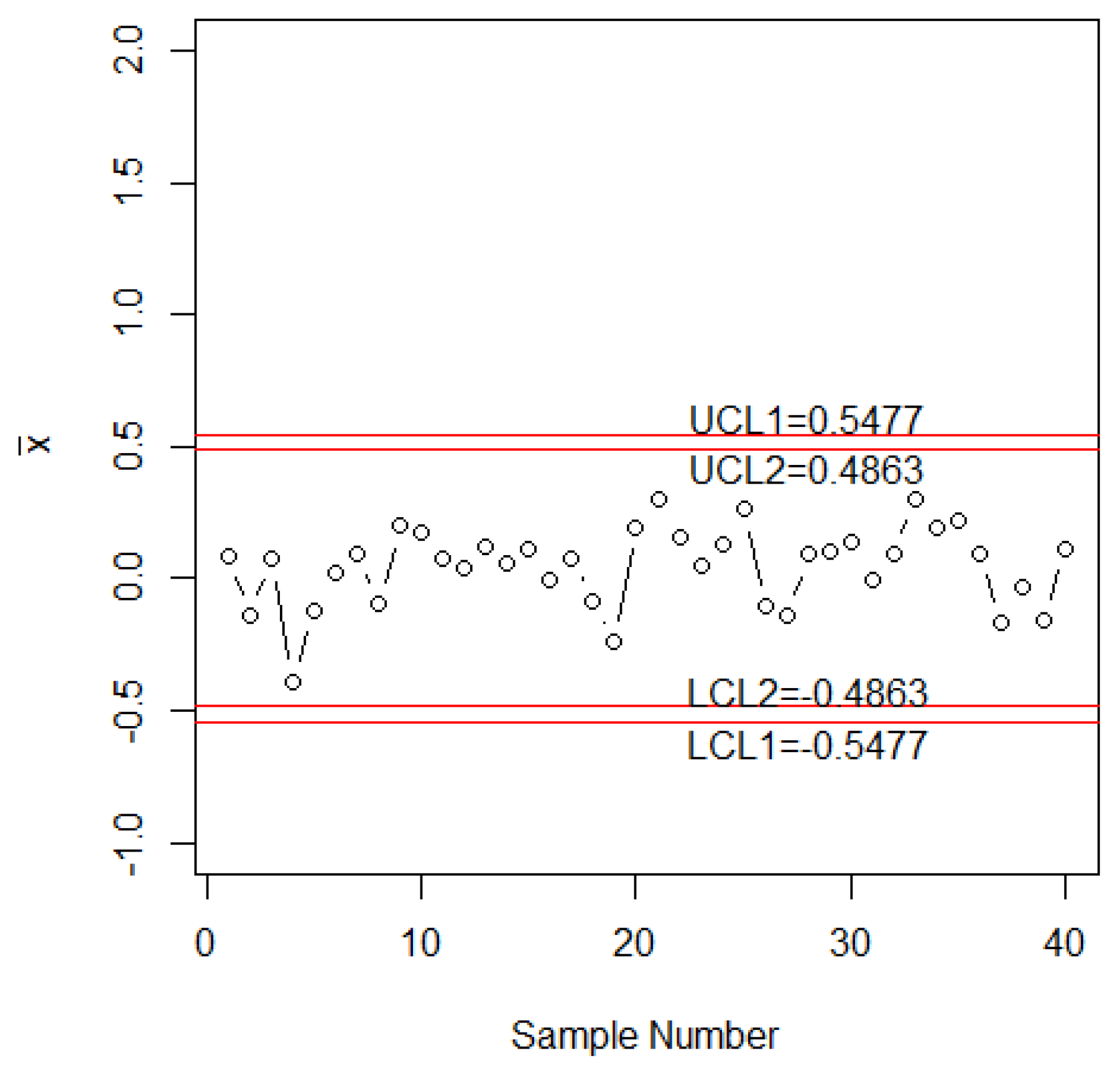
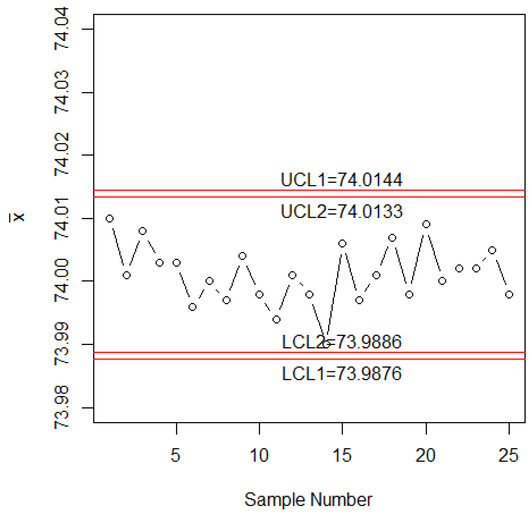
4. Industrial Application

In this section, the application of the proposed control chart will be explained with the aid of an industrial example taken from Reference [2]. The data is about inside diameter measurements of forged automobile engine piston rings [2]. Each sample or subgroup consists of five piston rings. For this application, let n = 5 and A R L 0 = 370. The control chart coefficients are k 1 = 2.9999 and k 2 = 2.7569. The four control limits are as: L C L 1 = 73.9875, L C L 2 = 73.9886, U C L 2 =74.0133 and U C L 1 =74.0144. The statistic X ¯ is plotted on Figure 3.
From Figure 3, it can be seen that the process is shown as in the control. However, it should be noted that some points are near to L C L 2 and U C L 2 .

5. Concluding Remarks

A new variable X-bar control chart using MDSR sampling is developed in this paper. The structure of the proposed chart is given. Some tables are given for practical applications in the industry. The efficiency of the proposed chart is discussed with the existing control charts. It is concluded that the proposed control chart performs better than the existing control charts in terms of ARLs. The proposed chart has the ability to detect a shift in the process faster when compared to existing control charts. Development of control charts using MDSR sampling under some other asymmetric distributions, and/or using other statistics such as an exponentially-weighted moving average (EWMA) can be considered for future study.

Author Contributions

Conceptualization, M.S.A., M.A., N.K. and C.-H.J.; methodology, M.S.A., M.A. and N.K.; software, M.S.A.; validation, C.-H.J.

Funding

This article was funded by the Deanship of Scientific Research (DSR) at King Abdulaziz University, Jeddah. The author, Muhammad Aslam, therefore, acknowledge with thanks DSR technical and financial support.

Acknowledgments

We are thankful to reviewers for their valuable suggestions.

Conflicts of Interest

The authors declare no conflict of interest.

References

  1. Shewhart, W.A. Statistical Method from the Viewpoint of Quality Control; Courier Corporation: North Chelmsford, MA, USA, 1939. [Google Scholar]
  2. Montgomery, D.C. Introduction to Statistical Quality Control; John Wiley & Sons: Hoboken, NJ, USA, 2017. [Google Scholar]
  3. Al-Oraini, H.; Rahim, M.A. Economic statistical design of X control charts for systems with Gamma (λ, 2) in-control times. Comput. Ind. Eng. 2002, 43, 645–654. [Google Scholar]
  4. Costa, A.F. X charts with variable sample size. J. Qual. Technol. 1994, 26, 155–163. [Google Scholar] [CrossRef]
  5. Chakraborti, S. Run length, average run length and false alarm rate of Shewhart X-bar chart: Exact derivations by conditioning. Commun. Stat. Simul. Comput. 2000, 29, 61–81. [Google Scholar] [CrossRef]
  6. Chen, G.; Cheng, S.W.; Xie, H. Monitoring process mean and variability with one EWMA chart. J. Qual. Technol. 2001, 33, 223–233. [Google Scholar] [CrossRef]
  7. He, D.; Grigoryan, A.; Sigh, M. Design of double-and triple-sampling X-bar control charts using genetic algorithms. Int. J. Prod. Res. 2002, 40, 1387–1404. [Google Scholar] [CrossRef]
  8. Baud-Lavigne, B.; Bassetto, S.; Penz, B. A broader view of the economic design of the X-bar chart in the semiconductor industry. Int. J. Prod. Res. 2010, 48, 5843–5857. [Google Scholar] [CrossRef]
  9. Safaei, A.S.; Kazemzadeh, R.B.; Niaki, S.T.A. Multi-objective economic statistical design of X-bar control chart considering Taguchi loss function. Int. J. Adv. Manuf. Technol. 2012, 59, 1091–1101. [Google Scholar] [CrossRef]
  10. LUPO, T. Economic-statistical design approach for a vssi X-bar chart considering taguchi loss function and random process shifts. Int. J. Reliab. Qual. Saf. Eng. 2014, 21, 1450006. [Google Scholar] [CrossRef]
  11. De Araújo Rodrigues, A.A.; Epprecht, E.K.; De Magalhães, M.S. Double-sampling control charts for attributes. J. Appl. Stat. 2011, 38, 87–112. [Google Scholar] [CrossRef]
  12. Aslam, M.; Khan, N.; Azam, M.; Jun, C.-H. Designing of a new monitoring t-chart using repetitive sampling. Inf. Sci. 2014, 269, 210–216. [Google Scholar] [CrossRef]
  13. Aslam, M.; Azam, M.; Jun, C.-H. A control chart for an exponential distribution using multiple dependent state sampling. Qual. Quant. 2014, 49, 455–462. [Google Scholar] [CrossRef]
  14. Aslam, M.; Nazir, A.; Jun, C.-H. A new attribute control chart using multiple dependent state sampling. Trans. Inst. Meas. Control 2014, 37. [Google Scholar] [CrossRef]
  15. Yen, F.Y.; Chong, K.M.B.; Ha, L.M. Synthetic-type control charts for time-between-events monitoring. PLoS ONE 2013, 8, e65440. [Google Scholar] [CrossRef] [PubMed]
  16. Abujiya, M.A.R.; Riaz, M.; Lee, M.H. Enhanced cumulative sum charts for monitoring process dispersion. PLoS ONE 2015, 10, e0124520. [Google Scholar] [CrossRef] [PubMed]
  17. Azam, M.; Aslam, M.; Jun, C.-H. Designing of a hybrid exponentially weighted moving average control chart using repetitive sampling. Int. J. Adv. Manuf. Technol. 2015, 77, 1927–1933. [Google Scholar] [CrossRef]
  18. Aslam, M.; Azam, M.; Jun, C.-H. New attributes and variables control charts under repetitive sampling. Ind. Eng. Manag. Syst. 2014, 13, 101–106. [Google Scholar] [CrossRef]
  19. Aslam, M.; Yen, C.-H.; Chang, C.-H.; Jun, C.-H. Multiple states repetitive group sampling plans with process loss consideration. Appl. Math. Model. 2013, 37, 9063–9075. [Google Scholar] [CrossRef]
  20. Aslam, M.; Khan, N.; Jun, C.-H. A Multiple Dependent State Control Chart Based on Double Control Limits. Research. J. Appl. Sci. Eng. Technol. 2014, 7, 4490–4493. [Google Scholar]
Figure 1. The proposed chart for simulated data.
Symmetry 10 00641 g001
Figure 2. The [18] chart for simulated data.
Symmetry 10 00641 g002
Figure 3. The proposed control chart for real data.
Symmetry 10 00641 g003
Table 1. Proposed chart when A R L 0 = 300 and i = 2 .
A R L 0 = 300
k12.93522.93522.93522.93522.93522.9352
k22.78652.78332.79192.78122.59912.6161
n51020304050
cARL1
0300.00300.00300.01300.00300.00300.00
0.01288.30282.96277.10269.77225.11222.28
0.02276.24265.44253.13239.19175.50170.96
0.05239.51213.87184.82159.0294.4388.13
0.1182.86143.06103.7478.0241.0635.77
0.15137.0694.6958.8339.9520.2716.70
0.2102.3863.3534.6121.7810.988.72
0.2576.7943.1721.2412.666.485.05
0.358.0630.0413.617.844.143.22
0.434.1815.516.333.602.121.71
0.521.008.723.462.071.401.22
0.613.475.322.191.441.131.05
0.79.013.521.581.171.031.01
0.86.282.501.281.061.011.00
0.94.561.901.121.021.001.00
13.441.541.051.001.001.00
Table 2. Proposed chart when A R L 0 = 300 and i = 3 .
A R L 0 = 300
k12.93522.93522.93522.93522.93522.9352
k22.74672.77972.79122.71452.57942.6090
n51020304050
c ARL1
0300.00300.00300.00300.00300.00300.00
0.01284.79282.54276.98257.00220.62220.58
0.02269.85264.70252.95219.69170.06168.94
0.05227.73212.66184.57137.7590.3586.70
0.1169.13141.91103.5766.3739.2635.20
0.15125.1193.8658.7334.3019.4716.47
0.292.9862.8034.5618.9810.608.62
0.2569.7042.8121.2111.206.295.00
0.352.7829.8013.597.044.043.20
0.431.2715.416.333.332.081.70
0.519.358.673.461.961.391.22
0.612.505.302.191.401.131.05
0.78.423.501.581.151.031.01
0.85.922.491.281.051.011.00
0.94.321.901.121.011.001.00
13.281.541.051.001.001.00
Table 3. Proposed chart when A R L 0 = 370 and i = 2 .
A R L 0 = 370
k12.99962.99962.99962.99962.99962.9997
k22.77842.79512.75912.74912.76322.6391
n51020304050
cARL1
0370.00370.00370.00370.00370.00370.00
0.01346.38339.78319.86307.08302.49257.71
0.02324.14311.40277.17256.48248.23191.57
0.05265.41238.15183.39154.64141.2694.73
0.1190.88152.1897.2272.7260.6337.77
0.15138.6598.7954.5737.1628.7617.49
0.2101.9365.5432.1720.3814.929.07
0.2575.8744.4719.8511.938.435.21
0.357.1630.8712.797.445.173.31
0.433.6015.886.033.472.451.74
0.520.668.903.332.021.531.23
0.613.265.422.131.421.181.06
0.78.893.571.551.161.051.01
0.86.202.531.261.051.011.00
0.94.511.921.111.011.001.00
13.401.551.051.001.001.00
Table 4. Proposed chart when A R L 0 = 370 and i = 3 .
A R L 0 = 370
k12.99962.99962.99962.99972.99972.9997
k22.75692.75782.70892.66372.56502.5805
n51020304050
cARL1
0370.00370.00370.00370.00370.00370.00
0.01343.64333.49308.33284.36245.12239.94
0.02319.36300.96260.24226.10178.94172.41
0.05257.47223.12165.07127.6389.3282.64
0.1182.55139.4986.0259.1738.1233.10
0.15131.8090.0948.4330.6618.9215.58
0.296.7059.8428.7817.1410.348.22
0.2571.9840.7617.9210.236.154.80
0.354.2828.4211.666.513.973.10
0.432.0214.775.593.142.061.67
0.519.768.363.141.891.381.20
0.612.745.132.041.361.121.05
0.78.573.411.511.141.031.01
0.86.012.441.241.041.011.00
0.94.381.871.101.011.001.00
13.321.521.041.001.001.00
Table 5. The comparisons of three charts when i = 2 ,   n = 5 and A R L 0 = 370.
c Proposed Chart[20] Chart[18] Chart
0.01346.38367.05358.73
0.02324.14362.37346.49
0.05265.41339.36306.20
0.10190.88282.19237.88
0.15138.65220.42179.15
0.20101.93166.80133.48
0.2575.87124.7999.50
0.3057.1693.3474.62
0.4033.6053.2543.13

