Parametric Blending of Triangular Meshes

Abstract

We present a new method for constructing a parametric blending surface that smoothly connects two triangular meshes. A user selects a subregion on each triangular mesh. The local parameterizations of two selected regions are found by using geodesic polar coordinates, and a base surface on each triangular mesh is constructed by two boundary curves on parametric domain. Finally, two base surfaces are smoothly blended for generating a blending surface. The shape of a blending surface can easily be controlled by several shape parameters or by directly manipulating surface point. We demonstrate the effectiveness of our technique by showing several modeling examples.

1. Introduction

Surface blending is a fundamental task in geometric modeling and computer-aided design. It constructs a smooth transition between intersecting or disjoint surfaces. Due to its usefulness, various techniques have been developed in the past few decades. However, most techniques have been mainly dealing with the blending of parametric surfaces or implicit surfaces, and thus the blending of polygonal meshes has been relatively neglected.

Hartmann [1] introduced an effective method for blending parametric curves and surfaces. Let ${\Gamma }_1(u,v)$ and ${\Gamma }_2(u,v)$ be two parametric surfaces. This method constructs a $G^n$ parametric blending surface $S(s,t)$ by a linear combination of two base surfaces $S_1(s,t)$ and $S_2(s,t)$, where $S_1(s,t)$ and $S_2(s,t)$ are reparametrized subpatches of ${\Gamma }_1(u,v)$ and ${\Gamma }_2(u,v)$, respectively. Song et al. [2] extended this technique by proposing practical methods for reparameterizing the base surfaces to be blended. However, these techniques [1,2] are essentially based on the parametric representation of ${\Gamma }_i(u,v)$, and thus direct application to triangular meshes would be a considerably challenging problem.

In this paper, we tackle this problem. Given two triangular meshes, ${\mathbb{M}}_1$ and ${\mathbb{M}}_2$, we construct two base surfaces, $S_1(\theta ,t)\subset {\mathbb{M}}_1$ and $S_2(\theta ,t)\subset {\mathbb{M}}_2$, and take their linear combination to produce a blending surface. In this process, the main difficulty lies in finding parametric representations of the base surfaces $S_1(\theta ,t)$ and $S_2(\theta ,t)$ on triangular meshes. To overcome this difficulty, we parameterized ${\mathbb{M}}_1$ and ${\mathbb{M}}_2$ and then constructed $S_1(\theta ,t)$ and $S_2(\theta ,t)$ based on these parameterizations. There exist a variety of sophisticated techniques for mesh parameterization [3,4,5,6,7,8]. 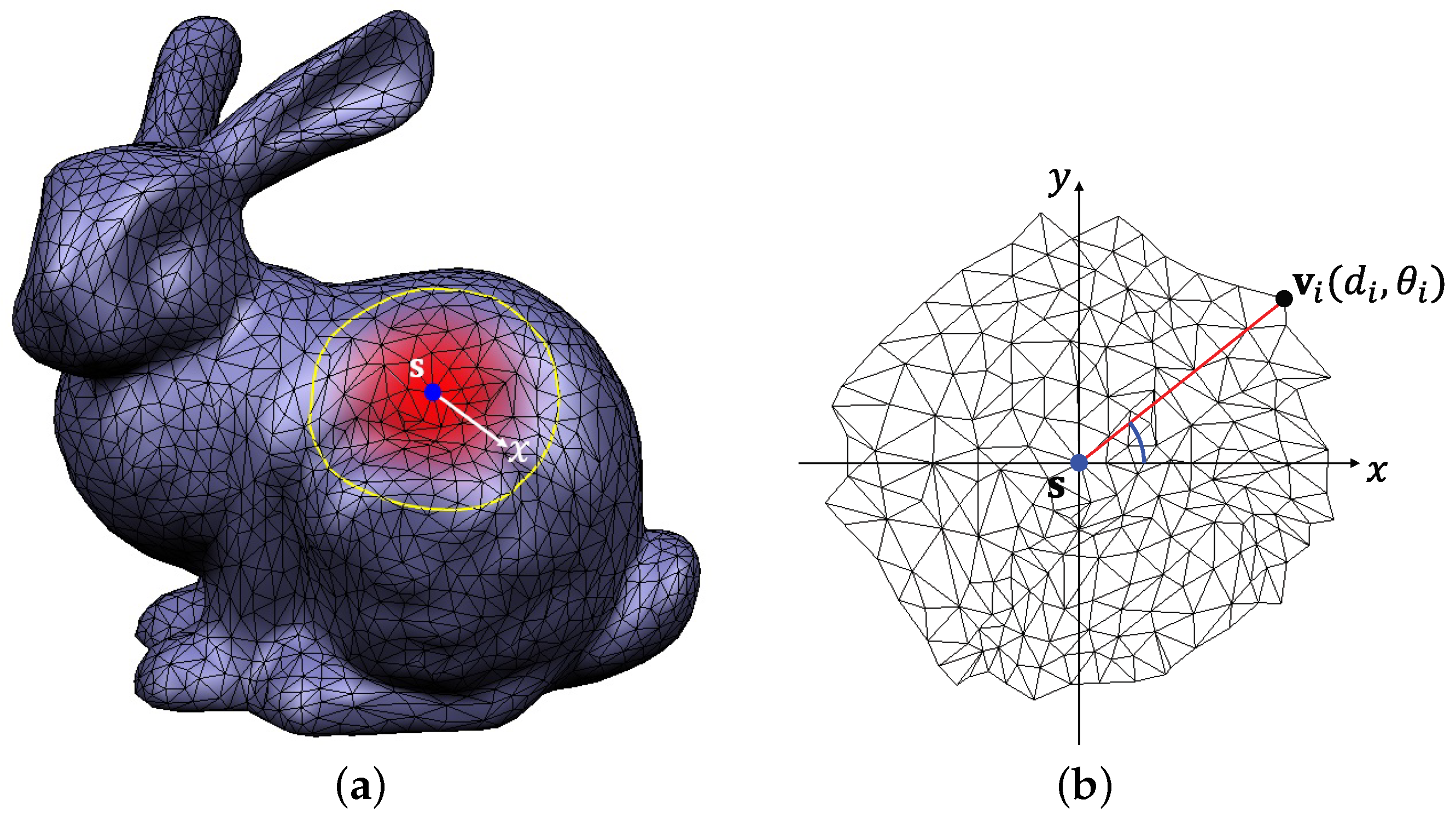Among them, we employed the efficient local parameterization method [8] based on geodesic polar coordinates. This method is quite suitable for our purpose since it uses a geodesic distance for common blending parameter t.

Figure 1 shows the overview of our method. First, a user specifies a local region on each triangular mesh (Figure 1a). 2D parameterization of the specified region is found, and two boundary curves are marked on the parameterization (Figure 1b,c) shows the base surfaces reparameterized by two boundary curves and then the blending surface smoothly connecting two base surfaces is shown in Figure 1d. Our framework allows a user to interactively control the shape of a blending surface by editing boundary curves in Figure 1b or adjusting several shape parameters.

Figure 1. Overview of our method: (a) selection of local regions; (b) 2D parameterizations of (a); (c) two base surfaces; (d) blending surface connecting two regions.

The main contributions of this paper can be summarized as follows:

• We present a simple and effective method for generating a parametric blending surface that smoothly joins the local regions of two triangular meshes.
• Our method provides a user with several parameters for controlling the shape of a blending surface.
• We propose an intuitive control mechanism for the direct manipulation of a blending surface.

The rest of this paper is organized as follows. Section 2 reviews some related recent work on surface blending, and Section 3 presents how to generate a parametric blending surface that smoothly joins the local regions of triangular meshes. The direct-manipulation technique is detailed in Section 4. Experimental results are demonstrated in Section 5, and we conclude the paper and suggest some future work in Section 6.

2. Related Work

There exist various classifications of blending methods. Vida et al. [9] conducted a comprehensive survey of blending methods. According to the surface type that they produce, the existing methods can be classified into several types. For example, implicit blending and parametric blending produce the blending surfaces as implicit or parametric forms, respectively. In this paper, we focus on the blending methods that produce a parametric surface.

Choi and Ju [10] presented an effective method for generating a blending surface by using a rolling ball of constant radius. In this method, a rolling ball simultaneously comes into contact with two base surfaces and generates a blending surface. Farouki and Sverrisson [11] extended this method to freeform parametric surfaces to produce the blending surfaces of rational tensor-product representation, and further extensions [12,13] have been made by using variable radius. Although rolling-ball methods provide a simple and intuitive geometric description, it is not easy to find spine curve and trimming curves without numerical approximations. Moreover, these methods are less flexible since contact curves are entirely determined by the relative position of the two base surfaces and the radius of the rolling ball. Bloor and Wilson [14,15] employed partial differential equations to generate a blending surface. However, their method is quite complicated to implement.

Linear combination is different type of blending method that produces a parametric blending surface. Hartmann [1] generated a parametric $G^n$ blending surface by linear combination of base surfaces which are subpatches of input surfaces. This method is quite simple and efficient. Moreover, it offers various design parameters, such as balance and thumb weight, to control the shape of the resulting surface. However, this method requires reparameterizations of the base surfaces and thus only a few examples were experimentally demonstrated. Song and Wang [2] improved this method by providing several reparameterization schemes, and also enhanced the shape of the blending surface by minimizing its strain energy. Lee et al. [16] employed linear blending scheme to generate a smooth surface interpolating the vertices of a triangular mesh.

In this paper, we deal with the blending of triangular meshes. Therefore, direct adaptation of the mentioned methods [1,2,10,11,12,13] is not applicable without suitable parameterizations of input meshes. Mesh parameterization is a fundamental technique for various applications, such as texture mapping, remeshing, compression, and surface reconstruction. Sophisticated techniques [3,4,6,7,8] have been developed depending on specific purposes. For much broader reviews of mesh parameterization, we refer the reader to an excellent survey paper [5].

Here, we are mainly interested in local parameterization since we are dealing with the blending of partial regions of input meshes. Recently, Melvær and Martin [8] presented an efficient method for the 2D parameterization of a polygon mesh. From a source vertex, they compute geodesic distance and polar angle for each vertex and construct 2D parameterization of a local region within a given geodesic distance. This method is based on a propagation scheme and thus does not need to solve a linear system. By combining existing methods [1,8], we propose a practical method for constructing a parametric blending surface that smoothly joins two disjoint triangular meshes. In our method, geodesic distance is used as a common blending parameter between base surfaces, and therefore plays a crucial role in generating a blending surface with good geometric properties.

3. Parametric Blending Surface

This section presents a method for constructing a parametric blending surface that smoothly joins the local regions of two triangular meshes.

3.1. Local Parameterization Based on Geodesic Polar Coordinates

Let $\mathbf{s}$ be a source vertex of triangular mesh $\mathbb{M}$. We define an open neighborhood of $\mathbf{s}$ as follows:

$$N_r(\mathbf{s})=\left\{\mathbf{v}\right|d(\mathbf{s},\mathbf{v})<r,\mathbf{v}\in \mathbb{M}\},$$

(1)

where $d(\mathbf{s},\mathbf{v})$ is the geodesic distance to a vertex $\mathbf{v}$ from $\mathbf{s}$, and r is a user-specified distance. Our goal is to find local parameterization $P:N_r(\mathbf{s})\to U(\subset {\mathbb{R}}^2)$ based on geodesic polar coordinates. We took a similar approach proposed by Reference [8], but present a different algorithm for improving computational efficiency.

We select an arbitrary edge incident to $\mathbf{s}$ for x-axis (see Figure 2). The first step is to find the geodesic polar coordinates $(d_l,{\theta }_l)$, $l=1,2,\cdots ,n$ of one-ring neighbor vertices ${\mathbf{v}}_l$ of $\mathbf{s}$. Geodesic distances $d_l$ can directly be determined by the edge distances, and the corresponding polar angles ${\theta }_l$ can be computed as follows:

$${\theta }_1=0\mathrm{and}{\theta }_l={\theta }_{l-1}+{\alpha }_{l-1}\left(\frac{2\pi }{{\sum }_{k=1}^n{\alpha }_k}\right)\mathrm{for}l=2,3,\cdots ,n,$$

(2)

where ${\alpha }_l$ is the angle between two edges, ${\overline{\mathbf{sv}}}_l$ and ${\overline{\mathbf{sv}}}_{l+1(modn)}$, and the scale factor $2\pi /{\sum }_{k=1}^n{\alpha }_k$ is necessary since ${\sum }_{k=1}^n{\alpha }_k\ne 2\pi$ in general.

Figure 2. Computation of geodesic polar coordinates.

The next step is to find the geodesic polar coordinates $(d_i,{\theta }_i)$ of a vertex ${\mathbf{v}}_i$ distant from $\mathbf{s}$. We consider a triangle $T_{ijk}$ incident to ${\mathbf{v}}_i$ and assume that the geodesic polar coordinates $(d_j,{\theta }_j)$, and $(d_k,{\theta }_k)$ of ${\mathbf{v}}_j$ and ${\mathbf{v}}_k$ have already been found (see Figure 2). The basic idea is to find virtual source vertex ${\mathbf{s}}^{\prime }$ from which the distances to ${\mathbf{v}}_j$ and ${\mathbf{v}}_k$ are identical to $d_j$ and $d_k$, respectively. The geodesic polar coordinates $(d_i,{\theta }_i)$ of a vertex ${\mathbf{v}}_i$ can then be determined from ${\mathbf{s}}^{\prime }$. Let $d_{jk}$ be the distance to ${\mathbf{v}}_k$ from ${\mathbf{v}}_j$. Depending on the distances $d_j$, $d_k$ and $d_{jk}$, the virtual source vertex ${\mathbf{s}}^{\prime }$ may exist or not. If triangle inequality holds, i.e., $|d_j-d_k|\le d_{jk}\le d_j+d_k$, then ${\mathbf{s}}^{\prime }$ exists (see Figure 3a). In this case, we can find the geodesic distance $d_i$ by mapping the triangle $T_{ijk}$ onto the $xy$ plane. By computing the intersection of two circles of radii $d_k$ and $d_j$, we can find the co-ordinates $(s_x,s_y)$ of ${\mathbf{s}}^{\prime }$ as follows:

$$s_x=\frac{d_k^2-d_j^2-d_{jk}^2}{2d_{jk}},s_y=\sqrt{d_j^2-s_x^2}.$$

(3)

Similarly, the coordinates $(x_i,y_i)$ of ${\mathbf{v}}_i^{\prime }$ can be computed as follows:

$$x_i=\frac{d_{ki}^2-d_{ij}^2-d_{jk}^2}{2d_{jk}},y_i=-\sqrt{d_{ij}^2-x_i^2}.$$

(4)

Figure 3. Two configurations of a virtual source vertex ${\mathbf{s}}^{\prime }$ that (a) exists and (b) does not exist.

Then, the geodesic distance to ${\mathbf{v}}_i$ from $\mathbf{s}$ can be approximated as $d_i=\parallel {\mathbf{s}}^{\prime }-{\mathbf{v}}_i^{\prime }\parallel$, and polar angle ${\theta }_i$ can linearly be interpolated as follows:

$${\theta }_i=(1-\omega ){\theta }_j+\omega {\theta }_k,$$

(5)

where $\omega ={\theta }_{ji}/{\theta }_{jk}$ (see Figure 3a for ${\theta }_{jk}$ and ${\theta }_{ji}$). If triangle inequality fails, i.e., $d_{jk}<|d_j-d_k|$ or $d_{jk}>d_j+d_k$, then ${\mathbf{s}}^{\prime }$ does not exist (see Figure 3b). In this case, we chose the minimum distance for $d_i=min\{d_j+\parallel {\mathbf{v}}_i-{\mathbf{v}}_j\parallel ,d_k+\parallel {\mathbf{v}}_i-{\mathbf{v}}_k\parallel \}$, and the polar angle is determined as follows:

$${\theta }_i=\left\{\begin{array}{cc}{\theta }_j& \mathrm{if} d_i \mathrm{is} \mathrm{taken} \mathrm{to} \mathrm{be} d_j+\parallel {\mathbf{v}}_i-{\mathbf{v}}_j\parallel ,\hfill \\ {\theta }_k& \mathrm{otherwise}.\hfill \end{array}\right.$$

(6)

We repeated this process for all triangles incident to ${\mathbf{v}}_i$ and updated geodesic polar coordinates $(d_i,{\theta }_i)$ whenever a shorter geodesic distance is found. Figure 4 shows local parameterization obtained by propagating this process to the neighborhood of source vertex $\mathbf{s}$.

Figure 4. (b) Local parameterization of (a) neighborhood of source vertex $\mathbf{s}$.

3.2. Constructing Blending Surface

Let $P_1$ be a local parameterization of $N_{r_1}({\mathbf{s}}_1)$ in triangular mesh ${\mathbb{M}}_1$ and ${\varphi }_1(\theta )$ and ${\varphi }_2(\theta )$ be two closed curves on $P_1$ (see Figure 5a). We consider parameter region $R_1$, defined as follows:

$$R_1(\theta ,t)=(1-t){\varphi }_1(\theta )+t{\varphi }_2(\theta ) \mathrm{for} 0\le \theta \le 2\pi ,0\le t\le 1,$$

(7)

where ${\varphi }_i(\theta )=(r_i(\theta )cos\theta ,r_i(\theta )sin\theta )$. Figure 5a shows an example of parameter region bounded by ${\varphi }_1(\theta )$ and ${\varphi }_2(\theta )$, and Figure 5b shows the corresponding base surface $S_1(\subset {\mathbb{M}}_1)$ constructed by $S_1(\theta ,t)=P_1^{-1}(R_1(\theta ,t))$. Note that $S_1(\theta ,0)$ corresponds to the outer boundary and $S_1(\theta ,1)$ to the inner one, respectively. Similarly, the other base surface, $S_2(\subset {\mathbb{M}}_2)$, can be constructed by $S_2(\theta ,t)=P_2^{-1}(R_2(\theta ,t))$, where $P_2$ is a local parameterization of $N_{r_2}({\mathbf{s}}_2)$ in ${\mathbb{M}}_2$ and $R_2$ is a parameter region defined by two closed curves ${\varphi }_3(\theta )$ and ${\varphi }_4(\theta )$ (see Figure 5c,d).

Figure 5. Base surfaces (b) and (d) generated by boundary curves (a) and (b).

Now, parametric blending surface $S(\theta ,t)$ can be generated by a linear combination of $S_1(\theta ,t)$ and $S_2(\theta ,t)$, as follows:

$$S(\theta ,t)=f(t)S_1(\theta ,t)+(1-f(t))S_2(\theta ,t),$$

(8)

where $f(t)$ is a blending function with $f(0)=1$ and $f(1)=0$. The resulting surface $S(\theta ,t)$ is $G^n$-continuous if $f(t)$ satisfies the following property:

$$f^{(k)}(0)=f^{(k)}(1)=0 \mathrm{for} k=0,1,\cdots ,n,$$

(9)

where $f^{(k)}(t)$ is the k-th derivative of $f(t)$. Our method does not guarantee theoretical continuity since we are dealing with the blending of triangular meshes (linear approximation of a continuous surface). However, for visual smoothness, we employ the $C^2$ blending function $f_{\mu }(t)$, defined as follows:

$$f_{\mu }(t)=\frac{\mu {(1-t)}^3}{\mu {(1-t)}^3+(1-\mu )t^3},$$

(10)

where parameter $\mu (\in [0,1])$ controls the shape of the blending function as shown in Figure 6. Figure 7 shows an example of a parametric blending surface generated by the linear combination of two base surfaces, $S_1(\theta ,t)$ and $S_2(\theta ,t)$, in Figure 5b,d.

Figure 6. Blending function $f_{\mu }(t)$.

Figure 7. Example of a blending surface.

3.3. Local Trimming of Triangular Meshes

Once the blending surface has been constructed, the local regions of triangular meshes should be trimmed and then seamlessly merged with the blending surface. For trimming the local regions, it is necessary to find intersections of contact curves with triangular meshes. In this paper, we took an approach to trimming a local region of a triangular mesh in 2D parameter space. As shown in Figure 8a, the triangles inside or intersected with ${\varphi }_1(\theta )$ were trimmed in 2D parameter space while resulting in a hole. We created new triangles by connecting the boundary vertices of the hole with the points sampled on ${\varphi }_1(\theta )$ and finally obtained the trimmed triangular mesh as shown in Figure 8b.

Figure 8. Trimming the local region of a triangular mesh in 2D parameter space: (a) initial trimming; (b) construction of smooth boundary.

4. Shape Control of Blending Surface

This section presents how to control the shape of a blending surface. Obviously, parameter $\mu$ in blending function $f_{\mu }(t)$ can be used to control the shape of a blending surface. In addition to blending function $f_{\mu }(t)$, the boundary curves ${\varphi }_i(\theta )$ in Equation (7) can also be used to control the shape of a blending surface. Firstly, two contact curves $S(\theta ,0)(\subset {\mathbb{M}}_1)$ and $S(\theta ,1)(\subset {\mathbb{M}}_2)$ can directly be controlled by ${\varphi }_1(\theta )$ and ${\varphi }_4(\theta )$ since $S(\theta ,0)=P_1^{-1}({\varphi }_1(\theta ))$ and $S(\theta ,1)=P_2^{-1}({\varphi }_4(\theta ))$. Figure 9a shows a curve ${\varphi }_1(\theta )$ of rectangular shape and the resulting surface is shown in Figure 9b. Similarly, ${\varphi }_4(\theta )$ can control the contact curve of the other side of the blending surface. Note that ${\varphi }_2(\theta )$ and ${\varphi }_3(\theta )$ may influence the interior shape of a blending surface. However, it is not easy to obtain a desired shape of blending surface by controlling ${\varphi }_2(\theta )$ and ${\varphi }_3(\theta )$. In this paper, we propose a simple and effective method for choosing ${\varphi }_2(\theta )$ and ${\varphi }_3(\theta )$, as follows:

$${\varphi }_2(\theta )=\alpha {\varphi }_1(\theta ) \mathrm{and} {\varphi }_3(\theta )=\beta {\varphi }_4(\theta ),$$

(11)

where $0\le \alpha ,\beta \le 1$. Figure 5a,c shows the examples of ${\varphi }_2(\theta )$ and ${\varphi }_3(\theta )$ for different control (scale) parameters $\alpha =0.3$ and $\beta =0.2$, respectively. This approach allows us to control the shape of blending surface by adjusting $\alpha$ and $\beta$. Figure 10 shows two extreme cases of generating blending surfaces when $\alpha =\beta =0$ and $\alpha =\beta =1$ while keeping the shapes of contact curves.

Figure 9. Influence of (a) boundary curve ${\varphi }_1(\theta )$ on (b) the blending surface.

Figure 10. Two blending surfaces generated by setting (a) $\alpha =\beta =0$ and (b) $\alpha =\beta =1$.

For practical use, we further extended this control mechanism to the direct manipulation of the blending surface. If a user selects a point $\mathbf{p}=S({\theta }_0,t_0)$ on a blending surface and moves it to a new position $\mathbf{q}$, control parameters $(\alpha ,\beta ,\mu )$ should be automatically adjusted so that $S({\theta }_0,t_0)$ passes through $\mathbf{q}$. Thus, our direct manipulation reduces to the problem of minimizing the following functional with the control parameters $(\alpha ,\beta ,\mu )$:

$$arg\underset{0\le \alpha ,\beta ,\mu \le 1}{min}\parallel S(\alpha ,\beta ,\mu ;{\theta }_0,t_0){-\mathbf{q}\parallel }^2,$$

(12)

where $S(\alpha ,\beta ,\mu ;{\theta }_0,t_0)$ can be explicitly represented as follows:

$$\begin{array}{ccc}\hfill S(\alpha ,\beta ,\mu ;{\theta }_0,t_0)& =& f_{\mu }(t_0)S_1({\theta }_0,t_0)+(1-f_{\mu }(t_0))S_2({\theta }_0,t_0)\hfill \\ & =& f_{\mu }(t_0)P_1^{-1}\left(R_1({\theta }_0,t_0)\right)+(1-f_{\mu }(t_0))P_2^{-1}\left(R_2({\theta }_0,t_0)\right)\hfill \\ & =& f_{\mu }(t_0)P_1^{-1}\left((1-(1+\alpha )t_0){\varphi }_1({\theta }_0)\right)+(1-f_{\mu }(t_0))P_2^{-1}\left((1-(1+\beta )t_0){\varphi }_4({\theta }_0)\right).\hfill \end{array}$$

Optimal control parameters $(\widehat{\alpha },\widehat{\beta },\widehat{\mu })$ can be efficiently found by well-known optimization techniques such as the conjugate gradient method [17,18]. Our direct manipulation method restricts users’ displacements for $\mathbf{q}$. More specifically, target position $\mathbf{q}$ should be inside the volume bounded by two extreme shapes generated by setting $\alpha =\beta =0$ and $\alpha =\beta =1$, respectively. Figure 11 shows the blending surface directly manipulated by our method.

Figure 11. Direct manipulation of surface point $\mathbf{p}$ to $\mathbf{q}$ (deformed blending surface is rendered by wireframes).

5. Experimental Results

We have implemented our technique in C++ on an Intel(R) Core(TM) i7 4.2 GHz CPU with an 8 GB main memory and an NVIDIA GeForce GTX 1070 graphic card. Our technique shows real-time performance for generating blending surfaces and directly manipulating them. In this section, we demonstrate the effectiveness of our technique by showing several examples of blending surfaces.

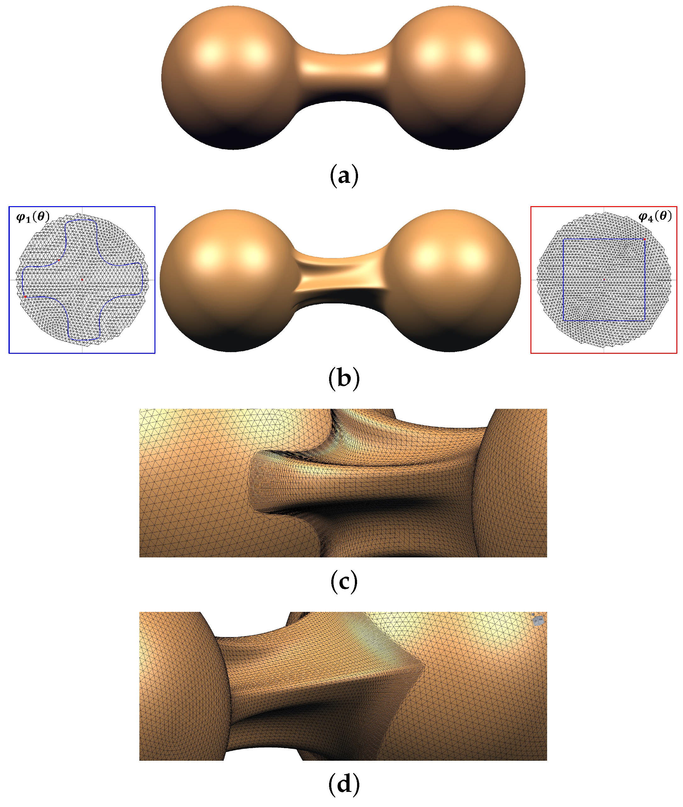
Figure 12a shows the blending surface that smoothly joins two sphere meshes. When we change the shape of boundary curves ${\varphi }_1(\theta )$ and ${\varphi }_4(\theta )$ as shown in Figure 12b, the blending surface changes its shape as shown in the middle figure. The result of merging the blending surface with trimmed meshes is detailed in Figure 12c,d.

Figure 12. Blending surfaces: (a) blending surface generated by circular contact curves; (b) blending surface generated by a cross-shaped contact curve and a rectangular contact one; (c,d): trimming results of the blending regions.

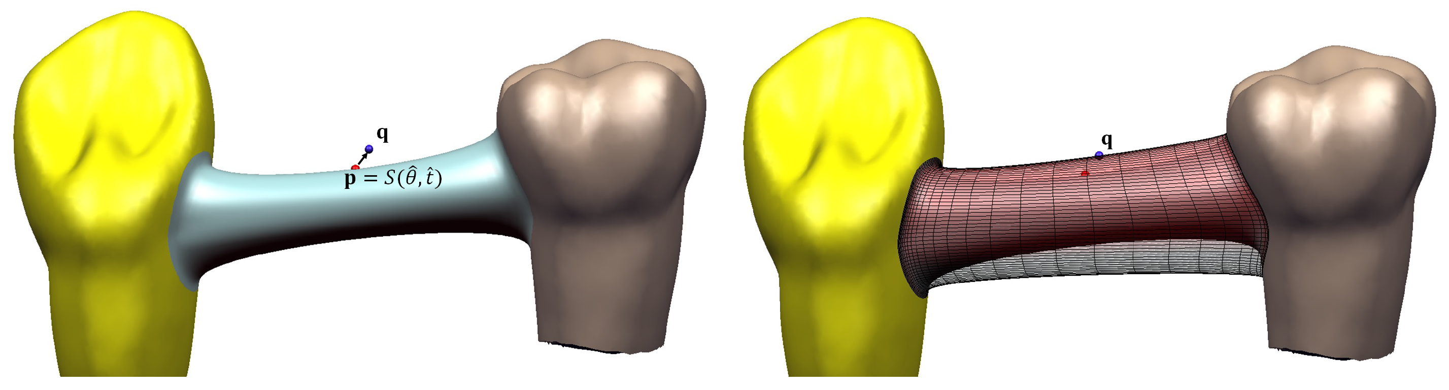
Figure 13 shows three blending surfaces joining two tooth models. Depending on parameter $\mu$ in the blending function, different shapes around contact regions are generated. As parameter $\mu$ gets closer to zero or one, the resulting surface becomes similar to the selected regions of triangular meshes. For visual inspection of the blending result, mean curvature is plotted in Figure 13d, where the middle part of the blending surface shows an almost constant curvature value. Figure 14 shows a boat steering wheel generated by our method. In Figure 14a, we positioned simple geometric primitives such as a sphere, torus, and ellipsoid in three-dimensional space, and twelve blending surfaces are then generated to smoothly connect these primitives.

Figure 13. Blending surfaces controlled by blending function $f_{\mu }(t)$: (a) $\mu =0.05$; (b) $\mu =0.5$; (c) $\mu =0.95$ and (d) mean curvature plots of (b).

Figure 14. (b) Blending surfaces smoothly join the (a) geometric primitives.

Similar to the rolling-ball methods [10,11,12,13], our method can also be used to generate a blending surface between two intersecting surfaces. Figure 15a,b shows two intersecting cylinders and the blending surface (in yellow) generated by using our method, respectively. Figure 15c shows the result of merging three surfaces after trimming unnecessary parts, and its 3D printing result without postprocessing is shown in Figure 15d. Compared with the rolling-ball methods, our method is more flexible for controlling the shape of the resulting surface. For example, the blending surface in Figure 15e is generated by setting ${\varphi }_2(\theta )={\varphi }_1(\theta )$ and ${\varphi }_3(\theta )=0.3{\varphi }_4(\theta )$. In Figure 15f, we use the boundary curves ${\varphi }_1(\theta )$ of rectangular shape and ${\varphi }_2(\theta )=0.5{\varphi }_1(\theta )$ to obtain the blending surface of a rectangular boundary curve. In rolling-ball methods, it would be quite difficult to control the shape of contact curves since they are automatically determined by the shape of the intersection curve between input meshes.

Figure 15. (a) Two intersecting cylinders; (b) blending surface connecting two cylinders; (c) merging three surfaces; (d) 3D printing of (c); (e, f) blending surfaces generated by different boundary curves.

Figure 16 shows various examples of blending surfaces. In Figure 16a, four nonintersecting cylinders of the same size are rotated about a common axis by different angles and the blending surfaces connecting adjacent cylinders are generated by our method. Figure 16b shows four intersecting cylinders of different sizes, orientations, and positions, and the blending surfaces between them are shown in Figure 16c. As shown in Figure 16, our method can robustly handle the various cases that can frequently occur in the geometric modeling process.

Figure 16. (a) Blending surfaces connecting separate cylinders; (c) blending surfaces connecting; (b) intersecting cylinders of arbitrary positions and orientations.

6. Conclusions

We have proposed a simple and effective method for constructing a parametric blending surface that smoothly connects two triangular meshes. For this, we combined two different geometric techniques: mesh parameterization and linear blending of parametric surfaces. The local regions of triangular meshes are parameterized by geodesic polar coordinates, and the corresponding base surfaces are constructed. By taking the linear combination of two base surfaces, we generated a blending surface. Our technique provides several parameters for controlling the shape of the blending surface. Moreover, our technique allows a user to control the blending result by directly manipulating surface points and also simultaneously deals with the blending of disjoint meshes and intersecting ones. In the experimental results, we have demonstrated the effectiveness of our technique by showing several modeling examples.

Compared with existing methods, it would be a strength of our method that finding the intersection curve between input meshes is not necessary, and sophisticated control of the boundary curve is possible. However, our method cannot deal with the case in which the blending region contains a hole. In this case, preprocessing for filling holes would be necessary. In future work, we plan to extend our method to include sophisticated parameters for controlling the shape of blending surfaces, and analyze geometric properties such as area and volume of the resulting surfaces.