Efficient Association Rules Hiding Using Genetic Algorithms

Abstract

In today’s world, millions of transactions are connected to online businesses, and the main challenging task is ensuring the privacy of sensitive information. Sensitive association rules hiding (SARH) is an important goal of privacy protection algorithms. Various approaches and algorithms have been developed for sensitive association rules hiding, differentiated according to their hiding performance through utility preservation, prevention of ghost rules, and computational complexity. A meta-heuristic algorithm is a good candidate to solve the problem of SARH due to its selective and parallel search behavior, avoiding local minima capability. This paper proposes simple genetic encoding for SARH. The proposed algorithm formulates an objective function that estimates the effect on nonsensitive rules and offers recursive computation to reduce them. Three benchmark datasets were used for evaluation. The results show an improvement of 81% in execution time, 23% in utility, and 5% in accuracy.

1. Introduction

Data mining is considered an influential technique to enhance decision-making, with several organizations and institutes using it to extract useful information and discover hidden patterns in datasets. This has made data mining a promising functional trend. Association rule mining (ARM) is an important data mining technique that extracts frequently co-occurring data items from transactional and relational databases and reveals hidden correlations between them. In a set of transactions, ARM focuses on finding associations between frequent items, enabling researchers to predict the frequency of one itemset depending on the frequency of another item in a transaction. The ARM technique has been extensively used in several applications, including privacy preservation [1], market-basket transaction data analysis [2], recommendation [3], health care [4,5], prediction [6], pattern finding in web browsing [7], ranking of text documents [8], and hazard identification [9], among others. The extraction of association rules from transaction datasets was initiated in 1993 [10]. A transaction dataset consists of a series of n-transactions D = (t₁, t₂, … t_n). Each transaction is a set of items I = {i₁, i₂ … i_m}, while the transaction is a pair comprising of an itemset and a unique transaction ID (TID, X). Itemset X is considered frequent if Supp (X) ≥ T_s, where T_s is the support threshold defined by the data miner. Supp (X) is the itemset support, which reflects the number of times itemset (X) occurs in the dataset. An association rule is presented as X ⇒ Y, where X and Y are two distinct sets of items. The rule X ⇒ Y shows that the presence of X suggests the presence of another Y in an identical transaction with certain confidence. To demonstrate this situation in a real-world scenario, we use the transaction dataset of a supermarket as an example, where the customer’s shopping list is a transaction. If a customer is buying “bread” and “butter,” then he will surely buy “milk”—the possible association rule is {bread, butter} ⇒ milk. More precisely, X ⇒ Y is considered as an association rule only if conf (X U Y) ≥ T_c and Supp (X U Y) ≥ T_s. We define conf (X U Y) as the confidence of X ⇒ Y, which is the ratio of the rule support over the left-hand side conf (X U Y) = Supp (X U Y)/Supp (X). T_c represents the confidence threshold determined by the data miner. The support and confidence threshold values of T_s and T_c are usually related to the category of the transaction, the usage of mining results, and the dataset size. Although ARM is the most effective data technique for mining the hidden patterns and associations between items, extracting this information without a breach in privacy is a challenging task. Private information, which is normally hidden in the dataset, can be disclosed on conducting a cross-analysis of multiple related datasets [11]; a major side effect of this process is the disclosure of sensitive information. Privacy has thus become a critical issue facing the data mining research community.

Association rule hiding (ARH) is a data mining technique used to preserve sensitive association rules. All ARH algorithms aim to minimally modify datasets such that no sensitive rule is extracted [12]. A hiding association rule can be regarded as a dataset inferential control, although it is concerned with protecting sensitive rules, not sensitive data [13]; it is the sensitive rule that causes the privacy breach.

In ARH, the number of sensitive association rules is determined by the dataset provider. Thus, when ARM algorithms are applied to that dataset, it can only extract nonsensitive rules. There have been other efforts (techniques) to hide sensitive association by modifying the original dataset. However, modifying the original dataset may have certain side effects, such as the loss of nonsensitive patterns (lost rule) or the creation of new rules (ghost rules).

Another technique, privacy preservation data mining (PPDM), has also gained considerable attention in transactional datasets [8]. PPDM maintains privacy by allowing the discovery of nonsensitive information and protecting sensitive information from disclosure.

The remainder of the paper is organized as follows: Section 2 provides a review of the literature. Section 3 describes the methodology used. Data description is provided in Section 4. Experimental results and analysis are given in Section 5. Finally, a conclusion and future work recommendations are given in Section 6.

2. Related Work

Association rule mining is the most extensively used (and promising) technique in the data mining field [14]. Since its introduction, it has created several opportunities to mine high-utility data [2]. It helps connect people with common interests [3] and provides new opportunities to improve public health and medicine; the prediction of post–liver transplantation survival is one example [4,5]. This technique helps users find documents relevant to their search [8] and potentially leads to beneficial services. However, privacy remains a critical issue [15].

Data sanitization strategies to preserve privacy are grouped into four categories: border-, exact-, evolutionary-, and heuristic-based algorithms. The border-based strategy specifies the revised positive and negative borders of all frequent itemsets. It focuses only on the weight of the maximin set [16] or positive border [17] to minimize the support of the changed negative border. The efficiency of the border-based algorithm was enhanced by formulating a hybrid algorithm called the decrease the confidence rule (DCR) based on the maximin approach. As the name suggests, the maximin approach uses two heuristics to hide the association rule [18], with the objective of controlling the sanitizing procedure aftereffects on the resulting quality by finding the victim items that are associated with the maximin solution. This is achieved by eliminating the victim item that has the shortest length. The intersection lattice of a frequent item approach for hiding association rules was mainly presented by Hai at el. [19,20]. These algorithms aim to conceal a specific set of sensitive rules in three steps. The first step specifies a set of itemsets satisfying three conditions: that they (i) contain a right-hand side of the sensitive rule, (ii) are a maximal sub-itemset of a maximal itemset, and (iii) have minimal support among those sub-itemsets specified in (ii). An item on the right-hand side of the sensitive rule that is related to the specified maximal support itemset is identified as the victim item. Second, the number of sensitive transactions is determined. Third, the victim items are deleted from the determined transactions until the confidence of the rule decreases below a specified minimum threshold. Finally, a number is assigned to all transactions to estimate the influence of the data hiding process on the nonsensitive association rules (NSARs) [21].

The exact approach [9] is considered as a constraint satisfaction problem to determine the best solution in the rule hiding process. It provides the least modification on the original dataset. Relatively, the exact approach provides more undesirable side effects than other approaches, but it suffers from high computational cost [9]. In recent years, many research studies have applied the evolutionary approach to hiding the frequent itemset.

Evolutionary algorithms are essentially inspired by Darwin’s evolutionary theory. The algorithms deal with populations of individuals in which all the individuals are possible candidate solutions for a particular problem to produce a better solution to that problem. The fitness function is used to measure the goodness of each solution. Some of the most interesting generic search algorithms proposed PGA2DT [22] and PS02DT [23] to solve the data hiding problem. The PGA2DT and PS02DT algorithms are based on the transaction deletion strategy, where a fitness function is designed to determine the suitable chromosomes for the minimum data sanitization process side effects. While all the chromosomes encode a solution consisting a number of transactions to be deleted, Lin et al. [24] used the genetic algorithm (GA) concept to determine possible associations for data sanitization. In chromosomes, all available genes represent potential candidates to be placed into a transaction. Three user-specific weights are assigned to three factors—hiding failure-sensitive high-utility itemsets, missing high-utility itemsets, and artificial high-utility itemsets—to evaluate the fitness values of chromosomes. The use of this algorithm reduces the computational time required for rescanning the original database compared to the simple GA-based algorithm. However, the authors used the approach of inserting new transactions, which affects the reliability of the generated dataset and might cause the generation of ghost rules.

The heuristic approach provides a useful and fast algorithm that chooses the suitable items in a specific transaction for hiding sensitive association rules using a distortion or blocking technique. The distortion technique inserts or deletes selected items of sensitive association rules from specified transactions or adds illegitimate transactions [25], to reduce the support [26] or confidence [27] of the rules under the given thresholds in order to hide single or multiple rules. Some research study investigated only changing the position of sensitive items in original data reduce the risk of data disclosure and balance the data confidentiality needs of the individual [28]. Chandra et al. [29] proposed an approach to select and alter the optimal transactions of a dataset to maintain the privacy and utility trade-off considering the Particle Swan Optimization (PSO) technique, which is a meta heuristic technique for solving complex optimization problems. Paratha et al. [30] adopted the heuristic strategy with an artificial bee colony algorithm to conceal the sensitive association rules. The experimental results showed zero failure of hiding the sensitive rules, lost rules, and high accuracy, although the work has some limitations, including the minimization of iterations. In this paper, we adopt the only alteration of the transaction through deletion techniques in order to avoid the formation of ghost rules. Furthermore, we formulate the approach in a simple genetic framework where each sensitive rule is concealed by calling the genetic algorithm to alter the set of transactions that have sensitive items in common with the rule. In this way, the genetic algorithm will be called only for the number of times equal to the sensitive rules, which assures lower computational cost. Moreover, the calculation of the objective function uses a recursive formula in order to guarantee low computational cost of the genetic execution.

In addition, artificial intelligence approaches were used to hide association rules. The research shows a fuzzy association rules hiding algorithm that was introduced to prevent the extraction of sensitive information from datasets while maintaining data utility [31]. In the algorithm, the support value of the item is decreased on either side of the rule in order to hide the sensitive rule. Some researchers investigated the up-to-date methodologies and compared the results. In their papers, the proposed algorithms achieved much better results for hiding failures, false rules, and reduced misses cost.

The existing approaches imply many solutions for hiding the sensitive rule observing the left-hand side (LHS) and right-hand side (RHS) of the rule as preserving the quality of the original database. However, recent studies show that the algorithm for hiding sensitive association rules suffers from high computational cost [18]; the problem arises when the transaction {g} ⇒ {e, c} supports the sensitive rule and supports the selected minimum confidence rule (MCR) {c} ⇒ {e, g}. Also, the border-based algorithm primarily focuses on privacy preservation, while the utility of the data is compromised [16]. Furthermore, as the evolutionary algorithms employ two transaction selection strategies—the transaction insertion [22] and insertion strategies [23,24]—these strategies revise the number of transactions of the dataset; for this reason, it is hard to extract patterns with an earlier minimum threshold.

3. Methodology

This section provides the developed methodology for sensitive association rule hiding (SARH). It starts with presenting the terms and symbols in Section 3.1. The problem formulation is given in Section 3.2. After that, we present efficient association rules hiding using a genetic algorithm (EARH-GA) in Section 3.3.

3.1. Terms and Symbols

This subsection provides the mathematical and algorithmic terms used in this paper, presented in

Table 1. Other notations.

Term	Meaning
AR	Set of association rules
SAR	Set of sensitive rules
NSAR	Set of nonsensitive rules
MC or ${\beta }_{\min }$	Minimum confidence threshold for hiding a sensitive rule
MS or ${\alpha }_{min}$	Minimum support threshold for hiding a sensitive rule
δ	Number of transactions to be altered with the object to hide the sensitive rule
VI	Set of victim items

.

3.2. Problem Formulation

Suppose we have the same database D from the previous section. After mining this database, we obtain the frequent itemsets and the association rules. We call the set of all association rules AR. There are two subsets of AR: SAR and NSAR. We are required to alter the set of transactions inside $D$ called $\mathrm{AT}=\left\{a{t}_1,a{t}_2,\dots ,a{t}_k\right\}$, where $\mathrm{AT}\subseteq D$, in order to conceal SAR. After this alteration, D is transformed to $D^{\prime }$. In $D^{\prime }$, all SARs have support or confidence lower than minimum support (MS) or minimum confidence (MC). Furthermore, we are required to conduct the alteration while assuring a minimum reduction of NSAR in order to maximize the utility of D. Other considerations are preventing ghost rules and assuring less computation time.

3.3. EARH-GA

Let us consider $X\subset {\mathcal{N}}^k$, where $x\in X,x=\left(x_1,x_2,\dots x_k\right)$, where $k$ indicates the set of transactions in $D^{\prime }$ that contains the victim item. $\mathcal{N}$ refers the number of positive integers. The solution space is set as $Y$, where each element $y\in Y,$ $y=\left(y_1,y_2,\dots y_{\delta }\right)$, where $S_y=\left\{y_1,y_2,\dots y_{\delta }\right\}\subset S_x=\left\{x_1,x_2,\dots x_k\right\}$. δ is the number of transactions to be altered with the aim of hiding the sensitive rule. If we have a rule X ⇒ Y, then δ is calculated by Equation (1):

$$\delta \left(X\Rightarrow Y\right)=\alpha \left(X\Rightarrow Y\right)-\mathrm{floor}\left(\mathrm{MC}\times \alpha \left(X\right)\right)$$

(1)

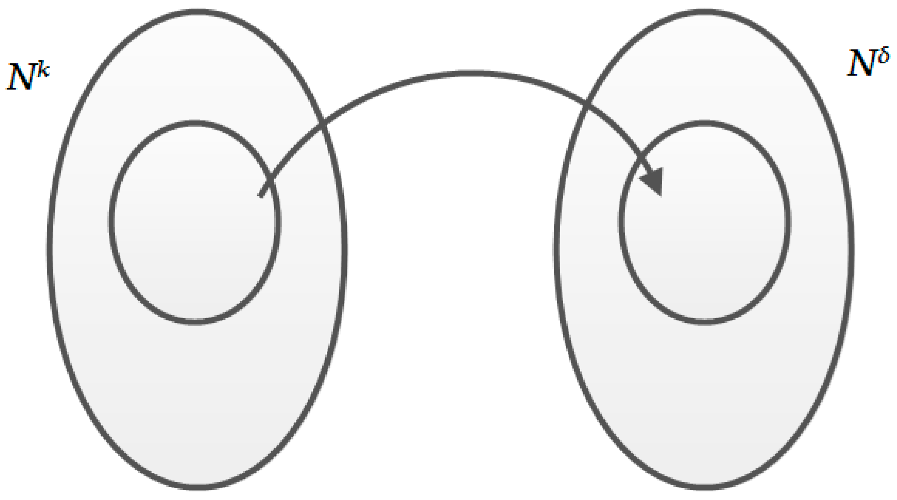
A Venn diagram that represents the relationship between $X$ and $Y$ is presented in Figure 1.

Two approaches are mostly used to alter the transaction, with the purpose of minimizing the confidence of sensitive rule X ⇒ Y below the MC. (1) Item deletion: this approach decreases the support count by considering the right-hand side (RHS) of rule Y by eliminating certain items, while the removed items from the sensitive transaction support both X and Y. (2) Item addition: this approach, on the other hand, increases the support count of the itemset on the left-hand side (LHS) of rule X. The support count is increased by adding items to the transactions containing X. In the first approach, a few nonsensitive rules may be hidden while all others are authentic. On the contrary, the second strategy may generate illegitimate rules in the sanitized database, and it may also fail to conceal the sensitive rules. Therefore, the item deletion approach has more benefit than item addition. The data sanitization process is aimed at protecting the sensitive knowledge against mining techniques, so in all the side effects, the hiding failure is more essential. Thus, we adopt this approach.

Genetic optimization is proposed to convert D to $D^{\prime }$. In order to achieve genetic optimization, two things have to be defined: the solution encoding and the objective function. The solution is encoded as a vector of indices that indicates the transactions that will be altered, while the objective function represents the ratio of the frequency of lost NSAR over the number of NSARs. The genetic algorithm will be called for the number of iterations of as many sensitive rules as we have. In each iteration, the algorithm deals with one sensitive association rule. First, in this step, our approach is to elect the victim item from the sensitive association rule. An item with minimum support of the RHS of the association rule is determined as the victim item, as such items produce fewer frequent itemsets and have minimum support. Therefore, the numbers of association rules containing the victim items have less frequency than other items, so deleting these items has a minor effect on nonsensitive association rules. Second, the algorithm will calculate $\delta$, the number of transactions that need to be altered using Equation (3). Third, it will select the transactions that contain the victim item as candidate transactions. Fourth, the GA will be called, and it should return the selected transaction. These are the transactions whose alteration will have the minimum impact on the nonsensitive rules, and their number is $\delta$. Finally, the algorithm will remove the victim item from the selected transaction according to the best solution, the database will be updated, and the algorithm will move on to the next SAR. Optimization association rule hiding using a genetic algorithm is presented in Algorithm 1. To elaborate on how the genetic algorithm works, we present the pseudocode in Algorithm 2. The genetic algorithm receives the DB′, which is the dataset that has to be altered. Also, it receives AR, SAR, CT, $\delta$, VI, MS, and MC. The result of the genetic algorithm is the selected transactions, which represent the algorithm’s global best solution. The operation of the genetic algorithm is described as a sequence of steps after initializing the population, which indicates the set of random vectors that belong to the set $X\subset N^{\delta }$, and the fitness values of the solutions will be evaluated using the fitness function, which is the number of lost NSARs over the number of NSARs when the solution is applied. Applying the solution means deleting the victim items from the selected transactions by the solution. A set of iterative steps is performed, and in each step, the elites are selected and used to produce offspring through two operations: crossover and mutation. In each iteration, the objective function will be called to evaluate the whole solution in the population.

Algorithm 1. Optimizing association rule hiding using a genetic algorithm.

Input: Database (DB), association rules (ARs), sensitive association rules (SARs), SARcounter = 0, minimum support (MS), minimum confidence (MC) Output: DB′ Start DB′ = DB While SARcounter < |SAR|     SARcounter = SARcounter + 1     for i = 1 to |items in the right-hand side of SAR|       itemSupport(i) = Support(DB′,item(i))     end     VI = the item with minimum itemSupport//VI indicates the victim item     $\delta$ = Support(DB′,SAR items) − floor (MC × Support (DB′, items in the left hand side of SAR))     candidateTransactions = transactions where victimItem belongs     selectedTransactions = GeneticAlgorithm(DB′, AR, SAR, NSAR, candidateTransactions, $\delta$, victimItem, MS, MC)     DB′ = Remove(selectedTransactions, victimItem, DB′) EndWhile End

Algorithm 2. The adopted genetic algorithm pseudocode.

Input: Database (DB′), association rules (ARs), sensitive association rule (SAR), nonsensitive association rules (NSARs), candidate transactions (CTs), $\delta$ victimItem (VI), MS, MC Output: Global best individual Start initialPopulation = initialize population randomly FitnessValues = objectiveFunction (initialPopulation, DB′, CT, VI, AR, NSAR, MS, MC, $\delta$) while (!stopCondition)     bestFitIndividuals = selectElite (FitnessValues)     newIndividuals = crossover and mutation (bestFitIndividuals)     FitnessValues = objectiveFunction(newIndividuals, DB′, CT, VI, AR, NSAR, MS, MC, $\delta$) endwhile globalBestIndividual = individual with min(FitnessValues) FitnessValues = objectiveFunction (Population, DB′, CT, VI, AR, NSAR, MS, MC, $\delta$) For each solution from Population     NewDB′ = DeleteVictim(DB′, VI, solution)     LostRules = FindLostRules(NewDB′, DB′)     LNSAR = FindLostNonSensitive(LostRules, NSAR)     FitnessValues.Add(LNSAR/NSAR) end End

3.4. Tracing Example

The goal of this example is to elaborate on the operation of the genetic algorithm. We present an example of a small dataset in

Table 2. Transaction dataset.

ID	Items
1	{l, m, n, r}
2	{m, o, p, q}
3	{l, m, n, t}
4	{l, o, p, q}
5	{l, m, n, t, r}
6	{m, p, r}
7	{l, m, n, o, p, q}
8	{n, o, q, t}

and all the following steps in order to obtain a new dataset for hiding a given sensitive rule.

Table 2 provides an example of a transaction database. Each dataset transaction comprises a set of items I = {a, b, c, d, e, f, g, h}, provided that the minimum support (MS) ${\alpha }_{min}$ = 37.5% and the minimum confidence (MC) ${\beta }_{min}$ = 75%. Twenty-four association rules are shown in

Table 3. Association rules.

Association Rule	Confidence
{l} ⇒ {m}	80%
{l} ⇒ {n}	80%
{n} ⇒ {l}	80%
{n} ⇒ {m}	80%
{p} ⇒ {m}	75%
{r} ⇒ {m}	100%
{t} ⇒ {n}	100%
{o} ⇒ {p}	75%
{p} ⇒ {o}	75%
{o} ⇒ {q}	75%
{q} ⇒ {o}	75%
{p} ⇒ {q}	75%
{q} ⇒ {p}	75%
{l} ⇒ {m, n}	80%
{n} ⇒ {l, m}	80%
{l, m} ⇒ {n}	100%
{l, n} ⇒ {m}	100%
{m, n} ⇒ {l}	100%
{o} ⇒ {p, q}	75%
{p} ⇒ {o, q}	75%
{q} ⇒ {o, p}	75%
{o, p} ⇒ {q}	100%
{o, q} ⇒ {p}	100%
{p, q} ⇒ {o}	100%

. These rules are the result of an a priori data mining algorithm [10]. Other popular ARM algorithms are FP-Growth [32] and Eclat [33].

If the rule {l} ⇒ {m, n} was chosen as a sensitive rule, then the victim item would be (n) because it has lower support compared to (m), where α(n) = 5 and α(m) = 6. Therefore, (n) should be removed from a certain number of transactions; this number is δ, which can be computed using Equation (2). So, altering one transaction is enough to hide the rule {l} ⇒ {m, n} and this is due to the small size of the dataset in our example. Let us suppose a dataset with 120 transactions whose support count of the rule is 98 (α (X ⇒ Y) = 98), the support count of itemset LHS of the rule is 102 (α (X) = 102), and the minimum confidence threshold is 0.75 (MC = 0.75), which can be formulated as Equation (3). Twenty-two transactions are sanitized; therefore, that it is possible the support count of itemset Y is reduced to 76, and thus the revised confidence of the rule would be 76/98 = 0.745.

$$\delta \left(X\Rightarrow Y\right)=(\alpha \left(X\Rightarrow Y\right)-\mathrm{floor} \left[\beta min\times \alpha \left(X\right)\right]$$

(2)

δ = 4 − floor [0.75 × 5] = 4 − floor (3.75) = 1

$$\delta =98-\mathrm{floor}\left(0.75\times 102\right)=22$$

(3)

Obtaining the best transactions is the result of applying a genetic algorithm, and the next section will demonstrate how this works.

Let us get back to the previous example, but with βmin = 50%, and with the sensitive rules (SARs) of {a} ⇒ {b, c} and {d, f} ⇒ {e}. First, we want to hide {a} ⇒ {b, c}; the victim item is (c), and δ is now 2 as computed using Equations (4) and (5). The sensitive rules are shown in

Table 4. Sensitive rules set.

Association Rule	Confidence
{l} ⇒ {m, n}	40%
{o, p} ⇒ {q}	100%

.

$$\delta \left(X\Rightarrow Y\right)=(\alpha \left(X\Rightarrow Y\right)-\mathrm{floor}\left[\beta min\times \alpha \left(X\right)\right]$$

(4)

$$\delta =4-\mathrm{floor}\left[0.5\times 5\right],\delta =4-\mathrm{floor}\left(2.5\right)=4-2=2$$

(5)

Candidate transactions support the sensitive rule, so they are the transactions with the IDs {1, 3, 5, 7} in the transaction dataset in Table 2, and they also represent the solution space for the genetic algorithm. The solution length (chromosome length) is 2 because δ = 2. If the population size is 4, then the initial generation would be something like: {1, 3} {5, 7} {1, 5} {3, 7}.

Next, the objective function in the equation is applied to each of these solutions. For example, for solution {1, 3}, if we delete (c) from transactions with IDs 1 and 3, the new dataset would be $D^{\prime }$, as shown in

Table 5. Updated transaction dataset $D^{\prime }$.

ID	Items
1	{l, m, r}
2	{m, o, p, q}
3	{l, m, t}
4	{l, o, p, q}
5	{l, m, n, t, r}
6	{m, p, r}
7	{l, m, n, o, p, q}
8	{n, o, q, t}

, and the new rules would be those shown in

Table 6. Nonsensitive rules set.

Association Rule	Confidence
{l} ⇒ {m}	80%
{l} ⇒ {n}	40%
{n} ⇒ {l}	66.66%
{n} ⇒ {m}	66.66%
{p} ⇒ {m}	75%
{r} ⇒ {m}	100%
{t} ⇒ {n}	66.66%
{o} ⇒ {p}	75%
{p} ⇒ {o}	75%
{o} ⇒ {q}	75%
{q} ⇒ {o}	75%
{p} ⇒ {q}	75%
{q} ⇒ {p}	75%
{n} ⇒ {l, m}	66.66%
{l, m} ⇒ {n}	50%
{l, n} ⇒ {m}	100%
{m, n} ⇒ {l}	100%
{o} ⇒ {p, q}	75%
{p} ⇒ {o, q}	75%
{q} ⇒ {o, p}	75%
{o, p} ⇒ {q}	100%
{p, q} ⇒ {o}	100%

.

The fitness value of this solution is #lost NSAR/#NSAR = 1/22. Let us say that the next solution has a fitness of (2/22, 5/22, 4/22). The next step is to select the elite individuals; the elite are the most important individuals to produce new individuals that are certain to survive to the next generation. The elite count is ceil (0.05 × population size). In our example, the elite count is ceil (0.05 × 4) = 1, and the elite individual is {1, 3} with a fitness of 1/22.

In order to elaborate the crossover and mutation, we assume two solutions—${\mathrm{S}}_{\mathrm{A}}=\left(1,2,6,4\right)$ and ${\mathrm{S}}_{\mathrm{B}}=\left(1,8,6,9\right)$—that contain the transactions that have to be altered. The crossover is done by generating one random vector with the same length as the parents; for example, $\mathrm{R}=\left(1,0,1,0\right)$. Then the child will inherit its genes from A in the case of 1 and from B in the case of 0: $\mathrm{Child}=\left(1,8,6,9\right)$. Following the crossover, mutation is performed, which provides a minor tweak to a chromosome to obtain diverse solutions. In this operation, first a ratio is chosen from the vector entries of an individual. All the entries of an individual have a probability rate of being mutated with a value of 0.01. In the next step, the selected entry of the individual is revised by a random number depending on the upper and lower limits for a particular entry. So, for a child with six entries (3, 6, 9, 1, 12, 5), the randomly selected fraction is 50%. Then entries (1, 2, 3) are checked with the mutation rate; if entry (3) is a hit, it will go to the second step and number (9) should be replaced by another random number selected uniformly by considering the upper and lower limits for this entry.

4. Dataset Description

Three datasets were used to conduct the experiments.

Table 7. Dataset descriptions.

Dataset	No. of Items	No. of Transactions	Transaction Length
Chess	75	3196	37
Mushroom	119	8124	23
Mobile	5250	5000	16

shows descriptions of the datasets: Chess, Mushroom, and Mobile. Two of the datasets are from the Irvine Machine Learning Repository. These datasets were originally generated and described in Reference [34]. In the Chess dataset, there are six attribute variables and one class variable. The second dataset is the Mushroom dataset, which contains 8124 records, each referring to a single mushroom. The label column represents the mushroom classification based on two categories: “edible” and “poisonous.” The other 22 columns are different features of mushrooms, such as color, shape, habitat, cape shape, gill size, and gill color. The third dataset is the Mobile dataset, which was prepared by our group. It is a huge dataset, so we took 5000 randomly chosen transactions to work on. This dataset has 16 columns, each one a feature, including location information, time, IP address, network performance, etc.

5. Experiments and Analysis

In this section, a set of comprehensive simulations and experiments are conducted to measure the efficiency of the proposed algorithm. In Section 5.1, an experimental setup is defined. In Section 5.2, we present the evaluation measure. In Section 5.2, we present the dataset description. Finally, in Section 5.3, we provide the evaluation results and their analysis.

5.1. Experimental Setup

Computational tests were conducted on three datasets for our experiments. The comparison of the benchmark and EARH-GA was analyzed in the same experimental context. The DCR and EARH-GA were implemented in MATLAB (2016a) and performed on an Intel Core i7 with 8 GB of RAM using the Windows 8 platform at 2.40 GHz. The Chess, Mushroom, and Mobile datasets were used to conduct the computational cost, and in the test case different confidence and support thresholds were applied to each repository.

5.2. Evaluation Measures

The first evaluation measure is execution time, which is used to prove the efficacy of the developed algorithm. The execution times of EARH-GA and DCR were calculated by observing the numbers of sensitive rules on the dataset.

Data utility and data accuracy are the evaluation metrics to estimate the effectiveness of the data sanitization algorithm. The effectiveness of a data sanitization algorithm is estimated by the capability to find the nonsensitive rules in the released dataset from the sanitized dataset. Clearly, data utility is associated with the number of lost rules in the original dataset. This implies that the data utility is determined to be high when there are fewer lost rules, and vice versa [18]. The data utility is calculated using Equation (6):

$$Data utility=1-\frac{number of lost rules}{number of rules}$$

(6)

Data accuracy is evaluated by determining the similarities between the original data and the sanitized datasets. Generally, it is the percentage of the number of items not removed from the sanitized dataset. It can be calculated as shown in Equation (7), where $D$ is an original dataset and $D^{\prime }$ is a sanitized dataset:

$$Accuracy=1-Dissimilarity\left(D,D^{\prime }\right)$$

(7)

To evaluate the accuracy of the sanitization algorithm, we should measure the dissimilarity. It is expressed as the difference between how many times an item appears in each dataset before and after the data sanitization process. It can be measured using Equation (8):

$$Dissimilarity\left(D,D^{\prime }\right)= \frac{{{\displaystyle \sum }}_{i=1}^m|f_D\left(i\right)-f_{D^{\prime }}\left(i\right)|}{{{\displaystyle \sum }}_{i=1}^n{f}_D\left(i\right)}$$

(8)

Misses cost is used to measure the side effects of the sanitization process. MC computes the percentage of lost rules that are hidden during the sanitization process. It can be measured using Equation (9):

$$Misses cost= \frac{f_D\left(i\right)-f_{D^{\prime }}\left(i\right)}{f_D\left(i\right)}$$

(9)

where D is the original dataset and $D^{\prime }$ is the sanitized dataset, m is the frequency of items in the dataset, $f_D\left(i\right)$ is the frequency of nonsensitive rules in the original dataset, and $f_{D^{\prime }}\left(i\right)$ is the frequency of nonsensitive rules in $D^{\prime }$. In order to maintain the quality of data, we need to reduce the number of missing nonsensitive rules as much as possible.

5.3. Performance Analysis

First, the data mining algorithm [10] was applied to these datasets using different values of support and confidence thresholds. Then, 1% of the resulting association rules were randomly chosen as sensitive rules. Finally, the two algorithms were used to hide the sensitive data and the following results were generated. We conducted several experiments for each dataset. In each experiment, the number of sensitive rules was constantly 1% and they were randomly chosen each time.

Table 8. Experimental settings of datasets.

Dataset	Minimum Confidence	No. of Association Rules	No. of Sensitive Rules
	94%	7177	72
Chess	95%	6145	62
	96%	4435	45
	97%	4081	41
	45%	4949	50
Mushroom	50%	4402	45
	55%	3937	40
	60%	3535	36
	40%	2092	20
	50%	1984	19
Mobile	60%	1801	18
	70%	1580	15
	80%	1333	13
	90%	1246	12

shows the different confidence thresholds during the association rules mining stage.

Figure 2a–c show the efficiency advantage of our approach compared to the DCR algorithm, where the execution time of EARH-GA and DCR are plotted against the confidence thresholds for the datasets. Execution time is a time duration taken by the algorithm to run a program. These increasing confidence thresholds resulted in a decreased number of sensitive rules and it is clear that less execution time is needed by the proposed algorithm as compared to the DCR for all datasets in all conditions.

Figure 3a–c show the utility in terms of the different number of sensitive rules for the three datasets. They demonstrate that EARH-GA has better utility compared to the DCR algorithm, as it has the lowest number of lost rules. However, the number of nonsensitive rules lost by the DCR was less than that of EARH-GA when the confidence threshold was 70 and 90 with the Mobile dataset. This resulted in worse utility in these two situations.

Figure 4a–c demonstrate the accuracy advantage of EARH-GA over the DCR, where in all tested situations our approach resulted in less dissimilarity and better accuracy. This comes back to the parallel nature of the GA when choosing the best solution.

Figure 5a–c demonstrate that with respect to different sizes of sensitive rules, EARH-GA has the lower misses count compared with the DCR algorithm. The misses cost of the proposed algorithm is less than that of the base algorithm.

All the experiments show that the proposed algorithm outperforms the DCR algorithm in all aspects. The performance improvement is elaborated in

Table 9. Percentage of improvement in results.

Improvement	Mushroom	Chess	Mobile	Max
Time	81%	70%	48%	81%
Lost rules ratio	36%	79%	21%	79%
Accuracy	5%	5%	3%	5%
Utility	2%	`2%	23%	23%

.

6. Conclusions

In this work, a novel algorithm called efficient association rules hiding using a genetic algorithm (EARH-GA) was presented for hiding sensitive association rules with better time cost while doing a better job of controlling the side effects of the nonsensitive rules. We managed to achieve this by taking advantage of the genetic algorithm and by using recursion in its objective function. With the objective of demonstrating the superiority of our approach, an algorithm called the decrease the confidence rule (DCR) was chosen as a benchmark. The experimental analysis demonstrated that the performance of EARH-GA was better than the DCR with regard to execution time, utility, and accuracy. In future work, we aim to develop the formulation of EARH-GA to consider hiding a set of rules in one optimization run instead of hiding one rule in every run.