New Stability Criterion for the Dissipative Linear System and Analysis of Bresse System

Abstract

In this article, we introduce a new approach to obtain the property of the dissipative structure for a system of differential equations. If the system has a viscosity or relaxation term which possesses symmetric property, Shizuta and Kawashima in 1985 introduced the suitable stability condition called in this article Classical Stability Condition for the corresponding eigenvalue problem of the system, and derived the detailed relation between the coefficient matrices of the system and the eigenvalues. However, there are some complicated physical models which possess a non-symmetric viscosity or relaxation term and we cannot apply Classical Stability Condition to these models. Under this situation, our purpose in this article is to extend Classical Stability Condition for complicated models and to make the relation between the coefficient matrices and the corresponding eigenvalues clear. Furthermore, we shall explain the new dissipative structure through the several concrete examples.

1. Introduction

We are interested in the profile of solutions for a system of differential equations. To investigate the profile, our first step is to analyze the eigenvalue of the corresponding linearized system. If the coefficient matrices of our system have a good property, it might be easy to analyze the eigenvalue problem. However, there are a lot of physical models which do not have enough properties to analyze the corresponding eigenvalue problem. (We will study several problems in Section 3 and Section 4). Under this situation, we focus on a general linear system with weak dissipation and try to construct the useful condition which induces the notable property of eigenvalues in this article.

Precisely, we consider a general linear system

$$A^0{u}_t+\sum _{j=1}^n{A}^j{u}_{x_j}-\sum _{j,k=1}^n{B}^{jk}{u}_{x_j{x}_k}+Lu=0.$$

(1)

Here, $u=u(t,x)$ over $t>0$, $x=(x_1,\cdots ,x_n)\in {\mathbb{R}}^n$ is an unknown vector function, and $A^0$, $A^j$, $B^{jk}$ and L are $m\times m$ constant matrices for $1\le j,k\le n$ and $m\ge 2$. Here and hereafter, we use notations that

$$A(\omega ):=\sum _{j=1}^n{A}^j{\omega }_j,B(\omega ):=\sum _{j,k=1}^n{B}^{jk}{\omega }_j{\omega }_k,$$

where $\omega =({\omega }_1,\cdots ,{\omega }_n)$ is a unit vector in ${\mathbb{R}}^n$, which means $\omega \in S^{n-1}$. Then, throughout this paper, we assume the following condition for the coefficient matrices of (1).

Condition (A):$A^0$ is real symmetric and positive definite, $A^j(1\le j\le n)$ are real symmetric, while $B(\omega )$ and L are not necessarily real symmetric but $B{(\omega )}^{♯}$ and $L^{♯}$ are non-negative definite with the non-trivial kernel for each $\omega \in S^{n-1}$.

Namely, Condition (A) means that the constant matrices satisfy the followings.

$$\begin{array}{c}{(A^j)}^T=A^j(0\le j\le n),\hfill \\ A^0>0,B{(\omega )}^{♯}\ge 0,L^{♯}\ge 0\mathrm{on}{\mathbb{R}}^m,\hfill \\ \mathrm{Ker}(B(\omega ))\ne \left\{0\right\},\mathrm{Ker}(L)\ne \left\{0\right\}\hfill \end{array}$$

for each $\omega \in S^{n-1}$. Here and in the sequel, the superscript T stands for the transposition, and $X^{♯}$ and $X^{♭}$ denote the symmetric and skew-symmetric part of the matrix X, respectively. That is $X^{♯}:=(X+X^T)/2$ and $X^{♭}:=(X-X^T)/2$. Furthermore, $m\times m$ real matrix X is called positive definite (resp. non-negative definite) on ${\mathbb{R}}^m$ if $(X^{♯}\phi ,\phi )>0$ (resp. $(X^{♯}\phi ,\phi )\ge 0$) for any $\phi \in {\mathbb{R}}^m\backslash \left\{0\right\}$, where $(·,·)$ denotes the standard real inner product in ${\mathbb{R}}^m$. Here, we remark that “ $X^{♯}$ is positive definite (resp. non-negative definite) on ${\mathbb{R}}^m$ ” is equivalent to $\langle X^{♯}\phi ,\phi \rangle >0$ (resp. $\langle X^{♯}\phi ,\phi \rangle \ge 0$) for any $\phi \in {\mathbb{C}}^m\backslash \left\{0\right\}$, and $\mathrm{Re}\langle X\phi ,\phi \rangle >0$ (resp. $\mathrm{Re}\langle X\phi ,\phi \rangle \ge 0$) for any $\phi \in {\mathbb{C}}^m\backslash \left\{0\right\}$, where $\langle ·,·\rangle$ denotes the standard complex inner product in ${\mathbb{C}}^m$. Furthermore, I and O denote an identity matrix and a zero matrix, respectively.

To analyze the dissipative structure of (1), we study the corresponding eigenvalue problem

$$\lambda A^0\phi +(irA(\omega )+r^{2}B(\omega )+L)\phi =0$$

(2)

for $r\ge 0$ and $\omega \in S^{n-1}$, and look for the eigenvalue $\lambda =\lambda (r,\omega )\in \mathbb{C}$ and the corresponding eigenvector $\phi =\phi (r,\omega )\in {\mathbb{C}}^m\backslash \left\{0\right\}$.

Remark 1.

Under Condition (A), the eigenvalues of (2) satisfy $\mathrm{Re}\lambda (r,\omega )\le 0$ for $r\ge 0$ and $\omega \in S^{n-1}$. In fact, using (2) and the symmetric property of $A^0$ and $A(\omega )$, we have

$$\mathrm{Re}\lambda \langle A^0\phi ,\phi \rangle +r^2\langle B{(\omega )}^{♯}\phi ,\phi \rangle +\langle L^{♯}\phi ,\phi \rangle =0$$

(3)

for each $r\ge 0$ and $\omega \in S^{n-1}$. Therefore, by the positivity of $A^0$ and non-negativity of $B{(\omega )}^{♯}$ and $L^{♯}$, we obtain the desired property.

We define the strict and uniform dissipativity for the system (1).

Definition 1.

(Strict and uniform dissipativity ([1])) (i) The system (1) is called strictly dissipative if the real part of all the eigenvalues of (2) is negative for each $r>0$ and $\omega \in S^{n-1}$. (ii) The system (1) is called uniformly dissipative of the type $(\alpha ,\beta )$ if all the eigenvalues $\lambda (r,\omega )$ of (2) satisfy

$$\mathrm{Re}\lambda (r,\omega )\le -c\frac{r^{2\alpha }}{{(1+r^2)}^{\beta }}$$

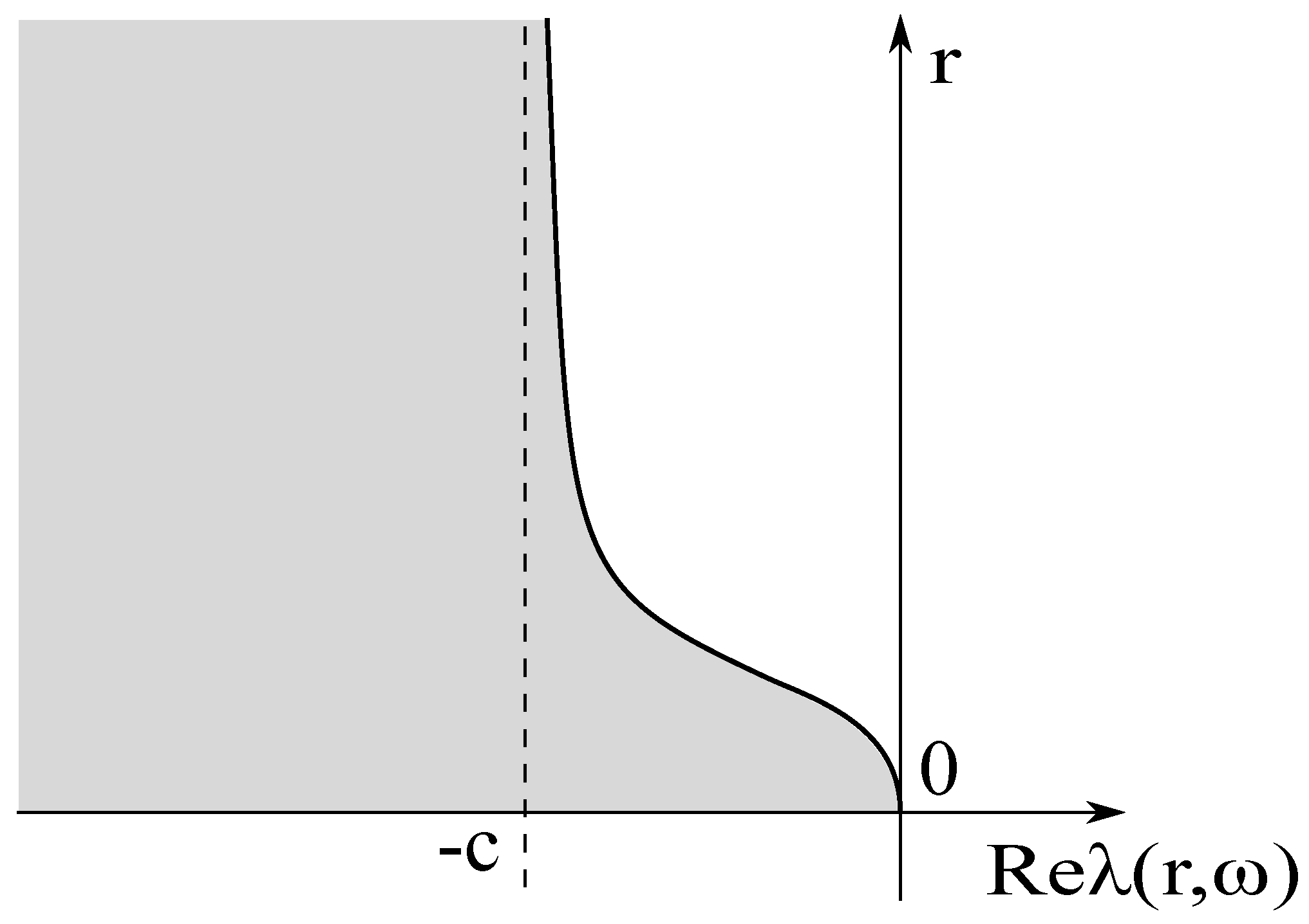
for each $r\ge 0$ and $\omega \in S^{n-1}$, where c is a certain positive constant and $(\alpha ,\beta )$ is a pair of non-negative integers.

Remark 2.

The uniform dissipativity of the type $(\alpha ,\beta )$ with $\alpha =\beta$ or $\alpha <\beta$ is called the standard type or the regularity-loss type, respectively.

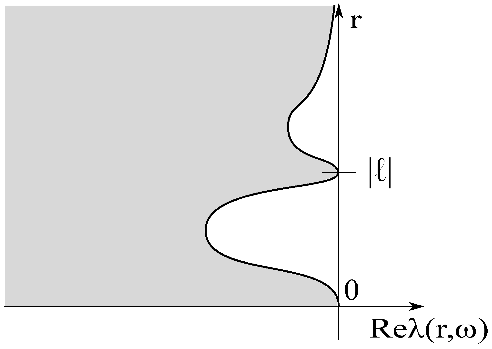
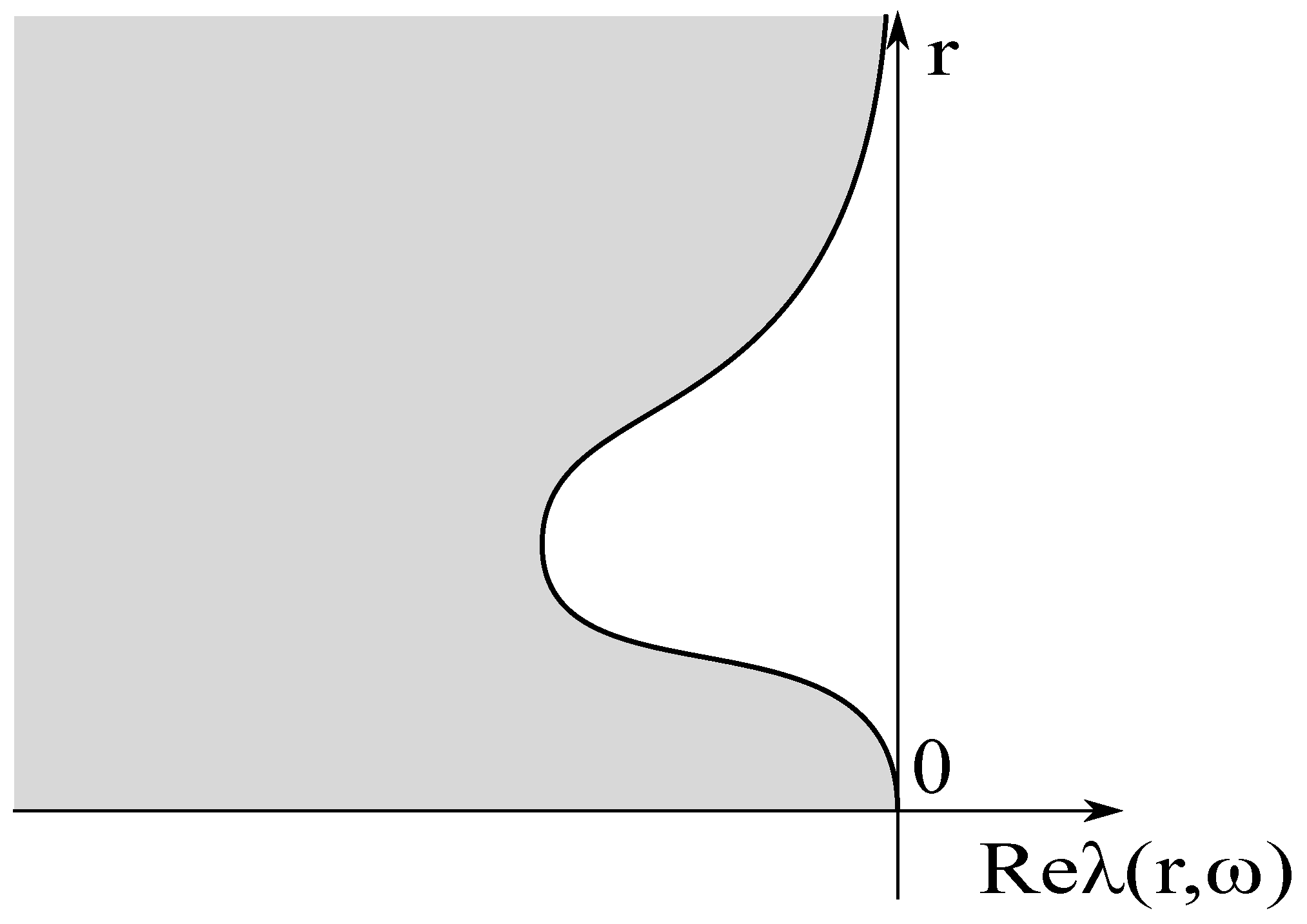
Remark that the vertical axis and the horizontal axis denote r and $\mathrm{Re}\lambda (r,\omega )$ for (2), respectively, in Figure 1, Figure 2 and Figure 3 appeared in Section 4. Under the strict dissipativity for the system (1), the real parts of the eigenvalues for (2) are located in the gray region in Figure 1 or Figure 2.

Under the symmetric property for $B(\omega )$ and L, Umeda et al. [2] and Shizuta and Kawashima [3] introduced the useful stability condition called Kawashima-Shizuta condition or Classical Stability Condition in this article. Precisely, they introduced the following conditions.

Classical Stability Condition (CSC): Suppose that $\mu A^0\phi +A(\omega )\phi =0$ and $\phi \in \mathrm{Ker}(B(\omega ))\cap \mathrm{Ker}(L)$ hold for each $(\mu ,\omega ,\phi )\in \mathbb{R}\times S^{n-1}\times {\mathbb{R}}^m$. Then $\phi =0$.

Condition (K): There is a real compensating matrix $K(\omega )\in C^{\infty }(S^{n-1})$ with the following properties: $K(-\omega )=-K(\omega )$, ${(K(\omega )A^0)}^T=-K(\omega )A^0$ and

$${(K(\omega )A(\omega ))}^{♯}>0\mathrm{on}\mathrm{Ker}(B(\omega ))\cap \mathrm{Ker}(L)$$

for each $\omega \in S^{n-1}$.

On the other hand, Kalman et al. [4], Coron [5] and Beauchard and Zuazua [6] discussed the different condition called Kalman Rank Condition for the system (1), that is as follows.

Classical Kalman Rank Condition (CR): For each $\omega \in S^{n-1}$, the $m^2\times m$ Kalman matrix has rank m, that is

$$\mathrm{rank}\left(\begin{array}{c}L\\ L{(A^0)}^{-1}A(\omega )\\ ⋮\\ L{({(A^0)}^{-1}A(\omega ))}^{m-1}\end{array}\right)=m.$$

Under this situation, the following theorem is obtained.

Theorem 1.

([2,3,6]) Suppose that the system (1) satisfies Condition (A) with

$$\mathrm{Ker}(B(\omega ))=\mathrm{Ker}(B{(\omega )}^{♯}),\mathrm{Ker}(L)=\mathrm{Ker}(L^{♯})$$

(4)

for each $\omega \in S^{n-1}$. Then, for the system (1), the following conditions are equivalent.

(i) 

System (1) is strictly dissipative.

(ii) 

System (1) is uniformly dissipative of the type $(1,1)$.

(iii) 

Condition (K) holds.

(iv) 

Classical Stability Condition (CSC) holds.

Furthermore, if $B^{jk}(1\le j,k\le n)$ is zero matrix, the above four conditions are equivalent to the following.

(v) 

Classical Kalman Rank Condition (CR) holds.

Remark 3.

Beauchard and Zuazua [6] considered the system (1) with $B^{jk}\equiv O$ for $1\le j,k,\le n$, and assumed that L satisfies

$$L=\left(\begin{array}{cc}O& O\\ O& L_1\end{array}\right),L_1\in {\mathbb{R}}^{m_1\times m_1},(L_1\phi ,\phi )>0\mathrm{for}\mathrm{any}\phi \in {\mathbb{R}}^{m_1}\backslash \left\{0\right\}.$$

(5)

We note that the assumption (5) is the sufficient condition for $L^{♯}\ge 0$ and $\mathrm{Ker}(L)=\mathrm{Ker}(L^{♯})$. Thus, we regard the assumption (5) as the essentially symmetric property. We will discuss in detail in Lemma 1. Emphasize that the physical examples in Section 4 do not satisfy (4) (and (5)).

We remark that the typical feature of the type $(1,1)$ is that the high-frequency part decays exponentially while the low-frequency part decays polynomially with the rate of the heat kernel (see Figure 1). A lot of physical models satisfy these conditions and can be treated by applying Theorem 1. For example, the model system of the compressible fluid gas and the discrete Boltzmann equation is studied by Kawashima [7] and Shizuta and Kawashima [3], respectively.

In recent 10 years, some complicated physical models which possess the weak dissipative structure called the regularity-loss structure was studied. For example, the dissipative Timoshenko system was discussed in [8,9,10], the Euler-Maxwell system was studied in [11,12], and the hybrid problem of plate equations is in [13,14,15,16]. We would like to emphasize that these physical models do not satisfy (4) but Condition (A). Namely, we can no longer apply Theorem 1 to these models. Under this situation, Ueda et al. [1] introduced the new condition called Condition (S) for the system (1) with $B^{jk}\equiv O(1\le j,k\le n)$ as follows.

Condition (S): There is a real compensating matrix S with the following properties: ${(S{A}^0)}^T=S{A}^0$ and

$${(SL)}^{♯}+L^{♯}\ge 0\mathrm{on}{\mathbb{R}}^m,\mathrm{Ker}({(SL)}^{♯}+L^{♯})\subseteq \mathrm{Ker}(L),$$

$$i{(SA(\omega ))}^{♭}=0\mathrm{on}\mathrm{Ker}(L^{♯})$$

for each $\omega \in S^{n-1}$.

Then they derived the sufficient condition which is a combination of Condition (K) and (S) to get the uniformly dissipativity of the type $(1,2)$, which is the regularity-loss type. We remark that the dissipative structure of the regularity-loss type is weaker than the one of the standard type. Precisely, $\mathrm{Re}\lambda (r,\omega )$ may tend to zero as $r\to \infty$ (see Figure 2). This structure requires more regularity for the initial data when we derive the decay estimate of solutions. This is the reason why this structure is called the regularity-loss type. Indeed, the dissipative Timoshenko system, the Euler-Maxwell system and the thermoelastic plate equation with Cattaneo’s law has the weak dissipative structure of type $(1,2)$. For the detail, we refer the reader to [8,9,11,12,16].

However, the stability condition constructed in [1] is not enough to understand the regularity-loss structure. In fact, some physical models which possess the regularity-loss structure do not satisfy the stability condition in [1] (e.g., [16,17,18]). Moreover, we can construct artificial models which have the several kinds of the regularity-loss structure (in detail, see [19]). Furthermore, in recent, Ueda et al. in [20] succeeded to extend Condition (K) and (S), and analyzed the more complicated dissipative structure.

This situation tells us that it is difficult to characterize the dissipative structure for the regularity-loss type. In fact, there is no related result. Under this situation, we try to extend Classical Stability Condition (CSC) and Classical Kalman Rank Condition (CR), and derive the sufficient and necessary conditions to get the strict dissipativity for (1) in Section 2. Furthermore, we will extend our main theorem to apply to a system under constraint conditions in Section 3. In Section 4, we introduce several physical models and apply our main theorems to them. Finally, we focus on the Bresse system as an interesting application of our main theorems in Section 5.

2. New Stability Criterion

We introduce the new stability condition for (1) in this section. The following conditions are important to characterize the dissipative structure for (1).

Stability Condition (SC): Suppose that

$$\begin{array}{c}\mu A^0\phi +(A(\omega )-i\nu B{(\omega )}^{♭}-i{\nu }^{-1}{L}^{♭})\phi =0,\hfill \\ \phi \in \mathrm{Ker}(B{(\omega )}^{♯})\cap \mathrm{Ker}(L^{♯})\hfill \end{array}$$

(6)

hold for each $(\mu ,\nu ,\omega ,\phi )\in \mathbb{R}\times {\mathbb{R}}_{+}\times S^{n-1}\times {\mathbb{C}}^m$. Then $\phi =0$.

Kalman Rank Condition (R): For each $(\nu ,\omega )\in {\mathbb{R}}_{+}\times S^{n-1}$, the $2m^2\times m$ Kalman matrix has rank m, that is

$$\mathrm{rank}\left(\begin{array}{c}B{(\omega )}^{♯}\\ B{(\omega )}^{♯}\mathcal{A}(\nu ,\omega )\\ ⋮\\ B{(\omega )}^{♯}\mathcal{A}{(\nu ,\omega )}^{m-1}\\ L^{♯}\\ L^{♯}\mathcal{A}(\nu ,\omega )\\ ⋮\\ L^{♯}\mathcal{A}{(\nu ,\omega )}^{m-1}\end{array}\right)=m.$$

Here and hereafter, we use notations that ${\mathbb{R}}_{+}:=(0,\infty )$ and

$$\mathcal{A}(\nu ,\omega ):={(A^0)}^{-1}(A(\omega )-i\nu B{(\omega )}^{♭}-i{\nu }^{-1}{L}^{♭})$$

for $(\nu ,\omega )\in {\mathbb{R}}_{+}\times S^{n-1}$. Under Stability Condition (SC) and Kalman Rank Condition (R), we can derive the following relation.

Theorem 2.

Suppose that the system (1) satisfies Condition (A). Then, for the system (1), the following conditions are equivalent.

(i) 

System (1) is strictly dissipative.

(ii) 

Stability Condition (SC) holds.

(iii) 

Kalman Rank Condition (R) holds.

Remark 4.

(i) If the matrices $B(\omega )$ and L satisfy (4), then Condition (SC) is equivalent to the Condition (CSC). Indeed, (4) and the second property of (6) give us $\phi \in \mathrm{Ker}(B{(\omega )}^{♭})\cap \mathrm{Ker}(L^{♭})$ for each $\omega \in S^{n-1}$. (ii) It is easy to check that the system (1) under Condition (A) satisfies Condition (CSC) if the system is strictly dissipative. Namely, Condition (SC) is sufficient condition for Condition (CSC).

To prove Theorem 2, we shall reduce our system. We introduce the new function $\tilde{u}:={(A^0)}^{1/2}u$. Then (1) is rewritten as

$${\tilde{u}}_t+\sum _{j=1}^n{\tilde{A}}^j{\tilde{u}}_{x_j}-\sum _{j,k=1}^n{\tilde{B}}^{jk}{\tilde{u}}_{x_j{x}_k}+\tilde{L}\tilde{u}=0,$$

(7)

where we define ${\tilde{A}}^j:={(A^0)}^{-1/2}{A}^j{(A^0)}^{-1/2}$, ${\tilde{B}}^{jk}:={(A^0)}^{-1/2}{B}^{jk}{(A^0)}^{-1/2}$ and $\tilde{L}:={(A^0)}^{-1/2}L{(A^0)}^{-1/2}$. Similarly as before, we use notations that

$$\tilde{A}(\omega ):=\sum _{j=1}^n{\tilde{A}}^j{\omega }_j,\tilde{B}(\omega ):=\sum _{j,k=1}^n{\tilde{B}}^{jk}{\omega }_j{\omega }_k.$$

Remark that the matrices of (7) satisfy Condition (A) if the matrices of (1) satisfy Condition (A). In this situation, the eigenvalue problem (2) is equivalent to

$$\lambda \tilde{\phi }+(ir\tilde{A}(\omega )+r^2\tilde{B}(\omega )+\tilde{L})\tilde{\phi }=0$$

(8)

with $\tilde{\phi }={(A^0)}^{1/2}\phi$.

For the problem (8), we consider the contraposition for Theorem 2. More precisely, we introduce the complement condition of Condition (SC) and $(\mathrm{R})$, and prove the contraposition of Theorem 2.

Condition (SC)${}^{\prime }$: There exist $({\mu }_0,{\nu }_0,{\omega }_0,{\tilde{\phi }}_0)\in \mathbb{R}\times {\mathbb{R}}_{+}\times S^{n-1}\times {\mathbb{C}}^m\backslash \left\{0\right\}$ such that

$$\begin{array}{c}\hfill ({\mu }_{0}I+\tilde{\mathcal{A}}({\nu }_0,{\omega }_0)){\tilde{\phi }}_0=0,{\tilde{\phi }}_0\in \mathrm{Ker}(\tilde{B}{({\omega }_0)}^{♯})\cap \mathrm{Ker}({\tilde{L}}^{♯}).\end{array}$$

(9)

Condition (R)${}^{\prime }$: There exist $({\nu }_0,{\omega }_0,{\tilde{\psi }}_0)\in {\mathbb{R}}_{+}\times S^{n-1}\times {\mathbb{C}}^m\backslash \left\{0\right\}$ such that

$${\tilde{\psi }}_0\in \bigcap _{k=0}^{m-1}\mathrm{Ker}(\tilde{B}{({\omega }_0)}^{♯}\tilde{\mathcal{A}}{({\nu }_0,{\omega }_0)}^k)\cap \mathrm{Ker}({\tilde{L}}^{♯}\tilde{\mathcal{A}}{({\nu }_0,{\omega }_0)}^k).$$

(10)

Here $\tilde{\mathcal{A}}(\nu ,\omega )$ is defined by $\tilde{\mathcal{A}}(\nu ,\omega ):=\tilde{A}(\omega )-i\nu \tilde{B}{(\omega )}^{♭}-i{\nu }^{-1}{\tilde{L}}^{♭}.$ Then our purpose is to prove the following theorem.

Theorem 3.

Suppose that the system (7) satisfies Condition (A). Then, for the system (7), the following conditions are equivalent.

(i) 

System (7) is not strictly dissipative.

(ii) 

Condition (SC)${}^{\prime }$ holds.

(iii) 

Condition (R)${}^{\prime }$ holds.

Proof. 

We first prove (i) from (ii). Since Condition (SC)${}^{\prime }$, we obtain

$$i{\mu }_0{\nu }_0{\tilde{\phi }}_0+(i{\nu }_0\tilde{A}({\omega }_0)+{\nu }_0^2\tilde{B}({\omega }_0)+\tilde{L}){\tilde{\phi }}_0=0.$$

Therefore, $\lambda =i{\mu }_0{\nu }_0\in i\mathbb{R}$ is an eigenvalue of (8) with $r={\nu }_0$, $\omega ={\omega }_0$, and ${\tilde{\phi }}_0\in {\mathbb{C}}^m\backslash \left\{0\right\}$ is a corresponding eigenvector. This means that the system (7) is not strictly dissipative under Condition (SC)${}^{\prime }$.

Secondly, we lead (ii) from (i). We assume that the system (1) is not strictly dissipative. Namely, there exists $(r_0,{\omega }_0)\in {\mathbb{R}}_{+}\times S^{n-1}$ such that $\mathrm{Re}\lambda (r_0,{\omega }_0)=0$. Then we obtain from (3) that $\tilde{B}{({\omega }_0)}^{♯}\tilde{\phi }(r_0,{\omega }_0)=0$ and ${\tilde{L}}^{♯}\tilde{\phi }(r_0,{\omega }_0)=0$, where $\tilde{\phi }(r_0,{\omega }_0)\in \mathbb{C}\backslash \left\{0\right\}$ is a corresponding eigenvector of $\lambda (r_0,{\omega }_0)$. Thus we employ (8) and get

$$\lambda (r_0,{\omega }_0)\tilde{\phi }(r_0,{\omega }_0)+(i{r}_0\tilde{A}({\omega }_0)+r_0^2\tilde{B}{({\omega }_0)}^{♭}+{\tilde{L}}^{♭})\tilde{\phi }(r_0,{\omega }_0)=0.$$

This means that

$$-i{r}_0^{-1}\lambda (r_0,{\omega }_0)\tilde{\phi }(r_0,{\omega }_0)+(\tilde{A}({\omega }_0)-i{r}_0\tilde{B}{({\omega }_0)}^{♭}-i{r}_0^{-1}{L}^{♭})\tilde{\phi }(r_0,{\omega }_0)=0.$$

Therefore, putting ${\mu }_0=-i{r}_0^{-1}\lambda (r_0,{\omega }_0)$, ${\nu }_0=r_0$ and ${\tilde{\phi }}_0=\tilde{\phi }(r_0,{\omega }_0)$, Condition (SC)${}^{\prime }$ is obtained.

Next, we prove (iii) from (ii). Since (9), we have

$$\tilde{B}{({\omega }_0)}^{♯}\tilde{\mathcal{A}}({\nu }_0,{\omega }_0){\tilde{\phi }}_0={\mu }_0\tilde{B}{({\omega }_0)}^{♯}{\tilde{\phi }}_0=0,{\tilde{L}}^{♯}\tilde{\mathcal{A}}({\nu }_0,{\omega }_0){\tilde{\phi }}_0={\mu }_0{\tilde{L}}^{♯}{\tilde{\phi }}_0=0$$

for ${\tilde{\phi }}_0\in \mathrm{Ker}(\tilde{B}{({\omega }_0)}^{♯})\cap \mathrm{Ker}({\tilde{L}}^{♯})$. Hence, we obtain

$${\tilde{\phi }}_0\in \mathrm{Ker}(\tilde{B}{({\omega }_0)}^{♯}\tilde{\mathcal{A}}({\nu }_0,{\omega }_0))\cap \mathrm{Ker}({\tilde{L}}^{♯}\tilde{\mathcal{A}}({\nu }_0,{\omega }_0)).$$

Therefore, the induction argument gives

$${\tilde{\phi }}_0\in \bigcap _{k\in \mathbb{N}\cup \left\{0\right\}}\mathrm{Ker}(\tilde{B}{({\omega }_0)}^{♯}\tilde{\mathcal{A}}{({\nu }_0,{\omega }_0)}^k)\cap \mathrm{Ker}({\tilde{L}}^{♯}\tilde{\mathcal{A}}{({\nu }_0,{\omega }_0)}^k).$$

Now, using the Cayley-Hamilton theorem, we have $g(\tilde{\mathcal{A}}({\nu }_0,{\omega }_0))=O$, where

$$g(\mu ):=det(\mu I-\tilde{\mathcal{A}}({\nu }_0,{\omega }_0)).$$

(11)

By virtue of $g(\tilde{\mathcal{A}}({\nu }_0,{\omega }_0))=O$, we derive (10) with ${\tilde{\psi }}_0={\tilde{\phi }}_0$.

Finally, we prove (ii) from (iii). Equation (11) is rewritten as

$$g(\mu )=det(\mu I-\tilde{\mathcal{A}}({\nu }_0,{\omega }_0))=\prod _{j=1}^m(\mu -{\tau }_j),$$

(12)

where ${\tau }_j\in \mathbb{R}$ since $\tilde{\mathcal{A}}({\nu }_0,{\omega }_0)$ is Hermitian matrix. If $m=2$, we consider the cases $(\tilde{\mathcal{A}}({\nu }_0,{\omega }_0)-{\tau }_{2}I){\tilde{\psi }}_0\ne 0$ or $(\tilde{\mathcal{A}}({\nu }_0,{\omega }_0)-{\tau }_{2}I){\tilde{\psi }}_0=0$, where ${\tilde{\psi }}_0$ is defined in Condition (R)${}^{\prime }$. When $(\tilde{\mathcal{A}}({\nu }_0,{\omega }_0)-{\tau }_{2}I){\tilde{\psi }}_0\ne 0$, we define ${\tilde{\psi }}_1:=(\tilde{\mathcal{A}}({\nu }_0,{\omega }_0)-{\tau }_{2}I){\tilde{\psi }}_0$. Then (12) gives $(\tilde{\mathcal{A}}({\nu }_0,{\omega }_0)-{\tau }_{1}I){\tilde{\psi }}_1=0$. Furthermore, it is easy to check ${\tilde{\psi }}_1\in \mathrm{Ker}(\tilde{B}{({\omega }_0)}^{♯})\cap \mathrm{Ker}({\tilde{L}}^{♯})$. Namely, ${\mu }_0=-{\tau }_1$ and ${\tilde{\phi }}_0={\tilde{\psi }}_1$ satisfy (9). On the other hand, when $(\tilde{\mathcal{A}}({\nu }_0,{\omega }_0)-{\tau }_{2}I){\tilde{\psi }}_0=0$, this gives (9) with ${\mu }_0=-{\tau }_2$ and ${\tilde{\phi }}_0={\tilde{\psi }}_0$. Using the induction argument, we can introduce $g_0(\mu )$ which is a divisor of $g(\mu )$ and define ${\tilde{\phi }}_0=g_0(\tilde{\mathcal{A}}({\nu }_0,{\omega }_0)){\tilde{\psi }}_0$ which satisfies (9) with ${\mu }_0=-{\tau }_0$, where ${\tau }_0$ is some eigenvalue of $\tilde{\mathcal{A}}({\nu }_0,{\omega }_0)$. Therefore, we complete the proof. □

Now, we study the relations between the conditions for (1) and the ones for (7). To this end, we focus on Condition $(\mathrm{R})$ and introduce the complement condition of Condition $(\mathrm{R})$ for (1) as follows.

Condition (R)${}^{″}$: There exist $({\nu }_0,{\omega }_0,{\psi }_0)\in {\mathbb{R}}_{+}\times S^{n-1}\times {\mathbb{C}}^m\backslash \left\{0\right\}$ such that

$${\psi }_0\in \bigcap _{k=0}^{m-1}\mathrm{Ker}(B{({\omega }_0)}^{♯}\mathcal{A}{({\nu }_0,{\omega }_0)}^k)\cap \mathrm{Ker}(L^{♯}\mathcal{A}{({\nu }_0,{\omega }_0)}^k).$$

Then we show that Condition (R)${}^{\prime }$ is equivalent to Condition (R)${}^{″}$. Indeed, Condition (R)${}^{\prime }$ means $\tilde{B}{({\omega }_0)}^{♯}\tilde{\mathcal{A}}{({\nu }_0,{\omega }_0)}^k{\tilde{\psi }}_0=0$ and ${\tilde{L}}^{♯}\tilde{\mathcal{A}}{({\nu }_0,{\omega }_0)}^k{\tilde{\psi }}_0=0$ for $0\le k\le m-1$. This is equivalent to

$$B{({\omega }_0)}^{♯}\mathcal{A}{({\nu }_0,{\omega }_0)}^k{(A^0)}^{-1/2}{\tilde{\psi }}_0=0,L^{♯}\mathcal{A}{({\nu }_0,{\omega }_0)}^k{(A^0)}^{-1/2}{\tilde{\psi }}_0=0$$

for $0\le k\le m-1$. Therefore, taking ${\psi }_0={(A^0)}^{-1/2}{\tilde{\psi }}_0$, Condition (R)${}^{″}$ is satisfied.

In the rest of this section, we study the relations between the assumption in Theorem 1 and (5).

Lemma 1.

Let X be $m\times m$ matrix and $m_1\le m$. Then,

$$X=\left(\begin{array}{cc}O& O\\ O& X_1\end{array}\right),X_1\in {\mathbb{R}}^{m_1\times m_1},(X_1\phi ,\phi )>0forany\phi \in {\mathbb{R}}^{m_1}\backslash \left\{0\right\}$$

(13)

is sufficient condition for

$$X^{♯}\ge 0,\mathrm{Ker}(X)=\mathrm{Ker}(X^{♯}).$$

Proof. 

Because of $(X_1^{♯}\phi ,\phi )/2=(X_1\phi ,\phi )>0$, it is easy to find $X^{♯}\ge 0$. Next, we assume $\mathrm{rank}(X_1)<m_1$. Then there is the regular matrix P such that $P{X}_1={\tilde{X}}_1$, where all of the components of the last column vector of ${\tilde{X}}_1$ is equal to zero. We introduce ${\phi }_0:=P^T{e}_{m_1}$, where $e_{m_1}:={(0,\cdots ,0,1)}^T$. This gives

$$(X_1{\phi }_0,{\phi }_0)=(P{X}_1{\phi }_0,{(P^T)}^{-1}{\phi }_0)=({\tilde{X}}_1{\phi }_0,e_{m_1})=0.$$

This fact is a contradiction under (13). Therefore, we obtain $\mathrm{rank}(X_1)=m_1$. Similarly as before, we also get $\mathrm{rank}(X_1^{♯})=m_1$, and hence $\mathrm{rank}(X_1)=\mathrm{rank}(X_1^{♯})$. Consequently, this yields $\mathrm{Ker}(X_1)=\mathrm{Ker}(X_1^{♯})$ which implies $\mathrm{Ker}(X)=\mathrm{Ker}(X^{♯})$. □

3. New Stability Criterion under Constraint Condition

In this section, we consider the system (1) under the constraint condition

$$\begin{array}{c}\sum _{j,k=1}^n{P}^{jk}{u}_{x_j{x}_k}+\sum _{j=1}^n{Q}^j{u}_{x_j}+Ru=0,\end{array}$$

(14)

where $P^{jk}$, $Q^j$ and R are $\tilde{m}\times m$ real constant matrices. In fact, a lot of physical models are described as (1) under (14). For example, the linearized system of the electro-magneto-fluid dynamics and Euler-Maxwell system are described as (1) under (14). For the detail, we refer [2,12] to the reader.

Similarly as before, we study the corresponding eigenvalue problem for the system (1) under the constraint condition (14). Namely, we look for the eigenvalue and the eigenvector of the eigenvalue problem (2) under the condition

$$(r^{2}P(\omega )-irQ(\omega )-R)\phi =0$$

(15)

for $r\ge 0$ and $\omega \in S^{n-1}$, where

$$P(\omega ):=\sum _{j,k=1}^n{P}^{jk}{\omega }_j{\omega }_k,Q(\omega ):=\sum _{j=1}^n{Q}^j{\omega }_j.$$

Here, we introduce a notation that

$${\mathcal{X}}_{r,\omega }:=\mathrm{Ker}(r^{2}P(\omega )-irQ(\omega )-R)$$

for $r\ge 0$ and $\omega \in S^{n-1}$. From this notation, (15) can be expressed as $\phi \in {\mathcal{X}}_{r,\omega }$. Then, the strict dissipativity and the uniform dissipativity under the constraint condition are defined as follows.

Definition 2.

(Strict dissipativity and uniform dissipativity under constraint) (i) The system (1) under the constraint condition (14) is called strictly dissipative under constraint if the real parts of the eigenvalues of (2), which eigenvectors are in ${\mathcal{X}}_{r,\omega }$, are negative for each $r>0$ and $\omega \in S^{n-1}$. (ii) The system (1) under the constraint condition (14) is called uniformly dissipative under constraint of the type $(\alpha ,\beta )$ if the eigenvalues $\lambda (r,\omega )$ of (2), which eigenvectors are in ${\mathcal{X}}_{r,\omega }$, satisfy

$$\mathrm{Re}\lambda (r,\omega )\le -c\frac{r^{2\alpha }}{{(1+r^2)}^{\beta }}$$

for each $r\ge 0$ and $\omega \in S^{n-1}$, where c is a certain positive constant and $(\alpha ,\beta )$ is a pair of non-negative integers.

Under the constraint condition (15), we introduce the modified stability condition and modified Kalman rank condition as follows.

Stability Condition under Constraint (SCC): Suppose that (6) and

$$({\nu }^{2}P(\omega )-i\nu Q(\omega )-R)\phi =0$$

(16)

hold for each $(\mu ,\nu ,\omega ,\phi )\in \mathbb{R}\times {\mathbb{R}}_{+}\times S^{n-1}\times {\mathbb{C}}^m$. Then $\phi =0$.

Kalman Rank Condition under Constraint (RC): For each $(\nu ,\omega )\in {\mathbb{R}}_{+}\times S^{n-1}$, the $(2m+\tilde{m})m\times m$ Kalman matrix has rank m, that is

$$\mathrm{rank}\left(\begin{array}{c}B{(\omega )}^{♯}\\ B{(\omega )}^{♯}\mathcal{A}(\nu ,\omega )\\ ⋮\\ B{(\omega )}^{♯}\mathcal{A}{(\nu ,\omega )}^{m-1}\\ L^{♯}\\ L^{♯}\mathcal{A}(\nu ,\omega )\\ ⋮\\ L^{♯}\mathcal{A}{(\nu ,\omega )}^{m-1}\\ \mathcal{R}(\nu ,\omega )\\ \mathcal{R}(\nu ,\omega )\mathcal{A}(\nu ,\omega )\\ ⋮\\ \mathcal{R}(\nu ,\omega )\mathcal{A}{(\nu ,\omega )}^{m-1}\end{array}\right)=m.$$

Here, we define $\mathcal{R}(\nu ,\omega ):={\nu }^{2}P(\omega )-i\nu Q(\omega )-R$. For these conditions, we obtain the following equivalence.

Theorem 4.

Suppose that the system (1) satisfies Condition (A). Then, for the system (1) under the constraint condition (14), the following conditions are equivalent.

(i) 

System (1) under (14) is strictly dissipative under constraint.

(ii) 

Condition (SCC) holds.

(iii) 

Condition (RC) holds.

The strategy of proof is almost the same as before. Namely, we consider the contraposition for (7) under (14) as follows.

Condition (SCC)${}^{\prime }$: There exist $({\mu }_0,{\nu }_0,{\omega }_0,{\tilde{\phi }}_0)\in \mathbb{R}\times {\mathbb{R}}_{+}\times S^{n-1}\times {\mathbb{C}}^m\backslash \left\{0\right\}$ such that (9) and $\tilde{\mathcal{R}}({\nu }_0,{\omega }_0){\tilde{\phi }}_0=0$.

Condition (RC)${}^{\prime }$: There exist $({\nu }_0,{\omega }_0,{\tilde{\psi }}_0)\in {\mathbb{R}}_{+}\times S^{n-1}\times {\mathbb{C}}^m\backslash \left\{0\right\}$ such that

$${\tilde{\psi }}_0\in \bigcap _{k=0}^{m-1}\mathrm{Ker}(\tilde{B}{({\omega }_0)}^{♯}\tilde{\mathcal{A}}{({\nu }_0,{\omega }_0)}^k)\cap \mathrm{Ker}({\tilde{L}}^{♯}\tilde{\mathcal{A}}{({\nu }_0,{\omega }_0)}^k)\cap \mathrm{Ker}(\tilde{\mathcal{R}}({\nu }_0,{\omega }_0)\tilde{\mathcal{A}}{({\nu }_0,{\omega }_0)}^k).$$

(17)

Here we defined that $\tilde{\mathcal{R}}(\nu ,\omega ):=\mathcal{R}(\nu ,\omega ){(A^0)}^{-1/2}$ and ${\tilde{\mathcal{X}}}_{r,\omega }:=\mathrm{Ker}(\tilde{\mathcal{R}}(\nu ,\omega ))$. Then we shall prove the following theorem.

Theorem 5.

Suppose that the system (7) satisfies Condition (A). Then, for the system (7) under the constraint condition (14), the following conditions are equivalent.

(i) 

System (7) under (14) is not strictly dissipative under constraint.

(ii) 

Condition (SCC)${}^{\prime }$ holds.

(iii) 

Condition (RC)${}^{\prime }$ holds.

Proof. 

Firstly, we prove (i) from (ii). Since Condition (SCC)${}^{\prime }$, we obtain

$$i{\mu }_0{\nu }_0{\tilde{\phi }}_0+(i{\nu }_0\tilde{A}({\omega }_0)+{\nu }_0^2\tilde{B}({\omega }_0)+\tilde{L}){\tilde{\phi }}_0=0.$$

Therefore, $\lambda =i{\mu }_0{\nu }_0\in i\mathbb{R}$ is an eigenvalue of (8) with $r={\nu }_0$, $\omega ={\omega }_0$, and ${\tilde{\phi }}_0\in {\mathbb{C}}^m\backslash \left\{0\right\}$ is a corresponding eigenvector. Furthermore, it is easy to find that ${\tilde{\phi }}_0\in {\tilde{\mathcal{X}}}_{r_0,{\omega }_0}$. Thus these facts tell us that the system (7) under the constraint condition (14) is not strictly dissipative in ${\tilde{\mathcal{X}}}_{r,\omega }$ under Condition (SCC)${}^{\prime }$.

Secondly, we prove (ii) from (i). We assume that the problem (1) under (14) is not strictly dissipative in ${\tilde{\mathcal{X}}}_{r,\omega }$. Namely, there exists $(r_0,{\omega }_0)\in {\mathbb{R}}_{+}\times S^{n-1}$ such that $\mathrm{Re}\lambda (r_0,{\omega }_0)=0$ and $\tilde{\phi }(r_0,{\omega }_0)\in {\tilde{\mathcal{X}}}_{r_0,{\omega }_0}$, where $(\lambda ,\tilde{\phi })$ is a pair of the eigenvalue and eigenvector of (8). Then we obtain from (3) that $\tilde{B}{({\omega }_0)}^{♯}\tilde{\phi }(r_0,{\omega }_0)=0$ and ${\tilde{L}}^{♯}\tilde{\phi }(r_0,{\omega }_0)=0$. Thus we employ (8) again and get

$$-i{r}_0^{-1}\lambda (r_0,{\omega }_0)\tilde{\phi }(r_0,{\omega }_0)+(\tilde{A}({\omega }_0)-i{r}_0\tilde{B}{({\omega }_0)}^{♭}-i{r}_0^{-1}{\tilde{L}}^{♭})\tilde{\phi }(r_0,{\omega }_0)=0.$$

Moreover, from the fact $\tilde{\phi }(r_0,{\omega }_0)\in {\tilde{\mathcal{X}}}_{r_0,{\omega }_0}$, this yields $\tilde{\mathcal{R}}(r_0,{\omega }_0)\tilde{\phi }(r_0,{\omega }_0)=0$. Finally, taking ${\mu }_0=-i{r}_0^{-1}\lambda (r_0,{\omega }_0)$, ${\nu }_0=r_0$ and ${\tilde{\phi }}_0=\tilde{\phi }(r_0,{\omega }_0)$ for the above relations, we conclude that Condition (SCC)${}^{\prime }$ is satisfied.

Thirdly, we prove (iii) from (ii). Since (9) and $\tilde{\mathcal{R}}({\nu }_0,{\omega }_0){\tilde{\phi }}_0=0$, we have

$$\begin{array}{c}\tilde{B}{({\omega }_0)}^{♯}\tilde{\mathcal{A}}({\nu }_0,{\omega }_0){\tilde{\phi }}_0={\mu }_0\tilde{B}{({\omega }_0)}^{♯}{\tilde{\phi }}_0=0,{\tilde{L}}^{♯}\tilde{\mathcal{A}}({\nu }_0,{\omega }_0){\tilde{\phi }}_0={\mu }_0{\tilde{L}}^{♯}{\tilde{\phi }}_0=0,\hfill \\ \tilde{\mathcal{R}}({\nu }_0,{\omega }_0)\tilde{\mathcal{A}}({\nu }_0,{\omega }_0){\tilde{\phi }}_0={\mu }_0\tilde{\mathcal{R}}({\nu }_0,{\omega }_0){\tilde{\phi }}_0=0\hfill \end{array}$$

for ${\tilde{\phi }}_0\in \mathrm{Ker}(\tilde{B}{({\omega }_0)}^{♯})\cap \mathrm{Ker}({\tilde{L}}^{♯})\cap \mathrm{Ker}(\tilde{\mathcal{R}}({\nu }_0,{\omega }_0))$. Hence, we obtain

$${\tilde{\phi }}_0\in \mathrm{Ker}(\tilde{B}{({\omega }_0)}^{♯}\tilde{\mathcal{A}}({\nu }_0,{\omega }_0))\cap \mathrm{Ker}({\tilde{L}}^{♯}\tilde{\mathcal{A}}({\nu }_0,{\omega }_0))\cap \mathrm{Ker}(\tilde{\mathcal{R}}({\nu }_0,{\omega }_0)\tilde{\mathcal{A}}({\nu }_0,{\omega }_0)).$$

Therefore, the same argument as in Theorem 3 gives (17).

Finally, we prove (ii) from (iii). We state the proof from (12) in Theorem 3. If $m=2$, we consider two cases that $(\tilde{\mathcal{A}}({\nu }_0,{\omega }_0)-{\tau }_{2}I){\tilde{\psi }}_0\ne 0$ or $(\tilde{\mathcal{A}}({\nu }_0,{\omega }_0)-{\tau }_{2}I){\tilde{\psi }}_0=0$. When $(\tilde{\mathcal{A}}({\nu }_0,{\omega }_0)-{\tau }_{2}I){\tilde{\psi }}_0\ne 0$, we define ${\tilde{\psi }}_1:=(\tilde{\mathcal{A}}({\nu }_0,{\omega }_0)-{\tau }_{2}I){\tilde{\psi }}_0$. Then (12) gives $(\tilde{\mathcal{A}}({\nu }_0,{\omega }_0)-{\tau }_{1}I){\tilde{\psi }}_1=0$. Furthermore, it is easy to check ${\tilde{\psi }}_1\in \mathrm{Ker}(\tilde{B}{({\omega }_0)}^{♯})\cap \mathrm{Ker}({\tilde{L}}^{♯})\cap \mathrm{Ker}(\tilde{\mathcal{R}}({\nu }_0,{\omega }_0))$. Namely, ${\mu }_0=-{\tau }_1$ and ${\tilde{\phi }}_0={\tilde{\psi }}_1$ satisfy (9) and $\tilde{\mathcal{R}}({\nu }_0,{\omega }_0){\tilde{\phi }}_0=0$. On the other hand, when $(\tilde{\mathcal{A}}({\nu }_0,{\omega }_0)-{\tau }_{2}I){\tilde{\psi }}_0=0$, this gives (9) and $\tilde{\mathcal{R}}({\nu }_0,{\omega }_0){\tilde{\phi }}_0=0$ with ${\mu }_0=-{\tau }_2$ and ${\tilde{\phi }}_0={\tilde{\psi }}_0$. Using the induction argument, we can introduce $g_0(\mu )$ which is a divisor of $g(\mu )$ and define ${\tilde{\phi }}_0=g_0(\tilde{\mathcal{A}}({\nu }_0,{\omega }_0)){\tilde{\psi }}_0$ which satisfies (9) and $\tilde{\mathcal{R}}({\nu }_0,{\omega }_0){\tilde{\phi }}_0=0$ with ${\mu }_0=-{\tau }_0$, where ${\tau }_0$ is some eigenvalue of $\tilde{\mathcal{A}}({\nu }_0,{\omega }_0)$. Hence, the proof is finished. □

Remark 5.

If $P(\omega )\equiv O$, $Q(\omega )\equiv O$ and $R\equiv O$, then ${\mathcal{X}}_{r,\omega }$ is equivalent to ${\mathbb{C}}^m$. Thus Condition (SCC) is equivalent to Condition (SC), and Theorem 4 is also equivalent to Theorem 2.

In the rest of this section, we discuss a relation for the constrain condition and the initial data. More precisely, we introduce the following condition.

Condition (C): The matrices $P(\omega )$, $Q(\omega )$ and R satisfy

$$\begin{array}{c}P(\omega ){(A^0)}^{-1}B(\omega )=0,P(\omega ){(A^0)}^{-1}A(\omega )-Q(\omega ){(A^0)}^{-1}B(\omega )=0,\hfill \\ P(\omega ){(A^0)}^{-1}L+Q(\omega ){(A^0)}^{-1}A(\omega )-R{(A^0)}^{-1}B(\omega )=0,\hfill \\ Q(\omega ){(A^0)}^{-1}L+R{(A^0)}^{-1}A(\omega )=0,R{(A^0)}^{-1}L=0\hfill \end{array}$$

for each $\omega \in S^{n-1}$.

Condition (C) implies the fact that (14) holds at an arbitrary time $t>0$ for the solution of (14) if it holds initially. For the detail, we refer the reader to [1]. Therefore, it is reasonable for the Cauchy problem to assign the constraint condition (14) which satisfies Condition (C). If we suppose that Condition (C) for the system (1) under (14), we can relax Condition (SCC).

Modified Stability Condition under Constraint (MSCC): Suppose that (6) hold for each $(\mu ,\nu ,\omega ,\phi )\in \mathbb{R}\backslash \left\{0\right\}\times {\mathbb{R}}_{+}\times S^{n-1}\times {\mathbb{C}}^m$. Then $\phi =0$. Furthermore, suppose that

$$(A(\omega )-i\nu B{(\omega )}^{♭}-i{\nu }^{-1}{L}^{♭})\phi =0,\phi \in \mathrm{Ker}(B{(\omega )}^{♯})\cap \mathrm{Ker}(L^{♯})$$

and (16) hold for each $(\nu ,\omega ,\phi )\in {\mathbb{R}}_{+}\times S^{n-1}\times {\mathbb{C}}^m$. Then $\phi =0$.

Theorem 6.

Under Condition (C), Condition (SCC) is equivalent to Condition (MSCC).

Proof. 

The sufficient condition is trivial. We only prove the necessary condition. Under Condition (C), this yields

$$({\nu }^{2}P(\omega )-i\nu Q(\omega )-R){(A^0)}^{-1}(i\nu A(\omega )+{\nu }^{2}B(\omega )+L)\phi =0$$

for each $(\nu ,\omega ,\phi )\in {\mathbb{R}}_{+}\times S^{n-1}\times {\mathbb{C}}^m$. Thus, by the first equation of (6), we get $-i\mu \nu ({\nu }^{2}P(\omega )-i\nu Q(\omega )-R)\phi =0$. Namely we arrive at (16) if $\mu \ne 0$, and complete the proof. □

Remark 6.

Theorem 6 tells us that if the system does not satisfy Condition (SC) for some $\mu \in \mathbb{R}\backslash \left\{0\right\}$, then it is difficult to find the useful constraint condition and apply Condition (SCC). On the other hand, if the system satisfies Condition (SC) for $\mu \ne 0$, it might be possible to find the useful constraint condition and apply Condition (SCC)(or (MSCC)) to the system. We will explain the situation by using concrete examples in Section 4.3, Section 4.4, Section 5.2 and Section 5.3.

4. Application to Physical Models

In this section, we introduce the several physical models for the application of Theorem 2, 4 and 6.

4.1. Timoshenko System

In this subsection, as an application of Theorems 2, we consider the following dissipative Timoshenko system

$$\left\{\begin{array}{c}{\varphi }_{tt}-{({\varphi }_x+\psi )}_x=0,\hfill \\ {\psi }_{tt}-a^2{\psi }_{xx}+({\varphi }_x+\psi )+\gamma {\psi }_t=0,\hfill \end{array}\right.$$

(18)

where a and $\gamma$ are positive constants, and $\varphi =\varphi (t,x)$ and $\psi =\psi (t,x)$ are unknown scalar functions of $t>0$ and $x\in \mathbb{R}$. The Timoshenko system above is a model system describing the vibration of the beam called the Timoshenko beam, and $\varphi$ and $\psi$ denote the transversal displacement and the rotation angle of the beam, respectively. Here we only mention [8,9] for related mathematical results.

As in [8,9], we introduce the vector function $u={({\varphi }_x+\psi ,{\varphi }_t,a{\psi }_x,{\psi }_t)}^T$. Then the Timoshenko system (18) is written in the form of (1) with coefficient matrices

$$A^0=I,A^1=\left(\begin{array}{cccc}0& -1& 0& 0\\ -1& 0& 0& 0\\ 0& 0& 0& -a\\ 0& 0& -a& 0\end{array}\right),B^{11}=O,L=\left(\begin{array}{cccc}0& 0& 0& -1\\ 0& 0& 0& 0\\ 0& 0& 0& 0\\ 1& 0& 0& \gamma \end{array}\right),$$

where I is the $4\times 4$ identity matrix and O is the $4\times 4$ zero matrix. Here the space dimension is $n=1$ and the size of the system is $m=4$. Notice that the relaxation matrix L is not symmetric. From the above matrices, we have

$$A(\omega )=\omega \left(\begin{array}{cccc}0& -1& 0& 0\\ -1& 0& 0& 0\\ 0& 0& 0& -a\\ 0& 0& -a& 0\end{array}\right)$$

for $\omega \in \{-1,1\}$, and the relaxation matrix L is decomposed $L=L^{♯}+L^{♭}$ with

$$L^{♯}=\left(\begin{array}{cccc}0& 0& 0& 0\\ 0& 0& 0& 0\\ 0& 0& 0& 0\\ 0& 0& 0& \gamma \end{array}\right),L^{♭}=\left(\begin{array}{cccc}0& 0& 0& -1\\ 0& 0& 0& 0\\ 0& 0& 0& 0\\ 1& 0& 0& 0\end{array}\right).$$

It is obvious that these matrices satisfy Condition (A), and we can apply Theorem 2 to the dissipative Timoshenko system.

Corollary 1.

The dissipative Timoshenko system (18) satisfies Condition (SC). Therefore, this system is strictly dissipative.

Proof. 

Condition (SC) states that $(\mu ,\nu ,\omega )\in \mathbb{R}\times {\mathbb{R}}_{+}\times \{-1,1\}$ and $\phi ={({\phi }_1,{\phi }_2,{\phi }_3,{\phi }_4)}^T\in {\mathbb{C}}^4$ satisfy

$$\left\{\begin{array}{c}\mu {\phi }_1-\omega {\phi }_2+i{\nu }^{-1}{\phi }_4=0,\hfill \\ \mu {\phi }_2-\omega {\phi }_1=0,\hfill \\ \mu {\phi }_3-a\omega {\phi }_4=0,\hfill \\ \mu {\phi }_4-a\omega {\phi }_3-i{\nu }^{-1}{\phi }_1=0,\hfill \end{array}\right.\mathrm{and}\gamma {\phi }_4=0.$$

Then, for any choice of $(\mu ,\nu ,\omega )\in \mathbb{R}\times {\mathbb{R}}_{+}\times \{-1,1\}$, we can get $\phi =0$. Namely, we conclude that the dissipative Timoshenko system (18) satisfies Condition (SC). This completes the proof of Corollary 1. □

4.2. Thermoelastic Plate Equation with Cattaneo’s Law

In this subsection, we consider the following linear thermoplastic plate equation in ${\mathbb{R}}^n$, where heat conduction is modeled by Cattaneo’s (Maxwell’s, Vernotte’s) law

$$\left\{\begin{array}{c}{v}_{tt}+{\Delta }^{2}v+\Delta \theta =0,\hfill \\ {\theta }_t+\mathrm{div}q-\Delta v_t=0,\hfill \\ \tau q_t+q+\nabla \theta =0.\hfill \end{array}\right.$$

(19)

Here, v describes the elongation of a plate, while $\theta$ and q denote the temperature and the heat flux, respectively. For Cattaneo’s law, the relaxation parameter $\tau$ is a positive constant. We have a lot of known results for the system (19). Especially, the system (19) is analyzed in detail by [16]. The authors of [16] obtained the sharp dissipative structure for the system (19), which is also regularity-loss structure.

We can rewrite (19) to a general system (1). To this end, we introduce new functions z and w as $z=\Delta v$ and $w=v_t$. Then our equation (19) can be rewritten as

$$\left\{\begin{array}{c}{z}_t-\Delta w=0,\hfill \\ w_t+\Delta z+\Delta \theta =0,\hfill \\ {\theta }_t+\mathrm{div}q-\Delta w=0,\hfill \\ \tau q_t+q+\nabla \theta =0.\hfill \end{array}\right.$$

(20)

Now, we introduce an unknown vector function $u={(z,w,\theta ,q)}^T$ and $n+3$ dimensional coefficient matrices $A^j$, $B^{jk}$ and L such that

$$\begin{array}{c}{A}^0=\left(\begin{array}{cccc}1& 0& 0& 0\\ 0& 1& 0& 0\\ 0& 0& 1& 0\\ 0& 0& 0& \tau I\end{array}\right),A(\xi )=\sum _{j=1}^n{A}^j{\xi }_j=\left(\begin{array}{cccc}0& 0& 0& 0\\ 0& 0& 0& 0\\ 0& 0& 0& {\xi }^T\\ 0& 0& \xi & 0\end{array}\right),\hfill \\ L=\left(\begin{array}{cccc}0& 0& 0& 0\\ 0& 0& 0& 0\\ 0& 0& 0& 0\\ 0& 0& 0& I\end{array}\right),B^{jk}=\left(\begin{array}{cccc}0& {\delta }_{jk}& 0& 0\\ -{\delta }_{jk}& 0& -{\delta }_{jk}& 0\\ 0& {\delta }_{jk}& 0& 0\\ 0& 0& 0& 0\end{array}\right),1\le j,k\le n,\hfill \end{array}$$

where I is the $n\times n$ identity matrix and ${\delta }_{jk}$ denotes Kronecker’s delta. Then the problem (20) can be rewritten as (1). Remark that the matrices $A^j$ and L are symmetric but $B^{jk}$ is skew-symmetric. From the above matrices, we get

$$A(\omega )=\left(\begin{array}{cccc}0& 0& 0& 0\\ 0& 0& 0& 0\\ 0& 0& 0& \omega \\ 0& 0& {\omega }^T& 0\end{array}\right),B(\omega )=\left(\begin{array}{cccc}0& 1& 0& 0\\ -1& 0& -1& 0\\ 0& 1& 0& 0\\ 0& 0& 0& 0\end{array}\right)$$

for $\omega \in S^{n-1}$. Under this situation, it is easy to check that our system satisfies Condition (A), and we can get the following property.

Corollary 2.

The thermoelastic plate equation with Cattaneo’s law (19) satisfies Condition (SC). Therefore, this system is strictly dissipative.

Proof. 

Condition (SC) suggests to state that $(\mu ,\nu ,\omega )\in \mathbb{R}\times {\mathbb{R}}_{+}\times S^{n-1}$ and $\phi ={({\phi }_1,{\phi }_2,{\phi }_3,{\phi }_4)}^T\in {\mathbb{C}}^{n+3}$ with ${\phi }_4\in {\mathbb{C}}^n$ satisfy

$$\left\{\begin{array}{c}\mu {\phi }_1-i\nu {\phi }_2=0,\hfill \\ \mu {\phi }_2+i\nu {\phi }_1+i\nu {\phi }_3=0,\hfill \\ \mu {\phi }_3+\langle {\phi }_4,\omega \rangle -i\nu {\phi }_2=0,\hfill \\ \mu \tau {\phi }_4+{\phi }_3{\omega }^T=0,\hfill \end{array}\right.\mathrm{and}{\phi }_4=0.$$

It is easy to check $\phi =0$ for any $(\mu ,\nu ,\omega )\in \mathbb{R}\times {\mathbb{R}}_{+}\times S^{n-1}$, and then we conclude that the thermoelastic plate equation with Cattaneo’s law satisfies Condition (SC). This completes the proof of Corollary 2. □

4.3. Coupled System of Wave and Heat Equations

We treat a coupled system of wave and heat equations as one of concrete examples in this subsection.

$$\left\{\begin{array}{cc}\hfill v_{tt}-\Delta v+a\theta & =0,\hfill \\ \hfill {\theta }_t-a{v}_t-\gamma \Delta \theta & =0.\hfill \end{array}\right.$$

(21)

Here $v=v(t,x)$ and $\theta =\theta (t,x)$ over $t>0$, $x\in {\mathbb{R}}^n$ are unknown scalar functions, and a and $\gamma$ denote constants which satisfy $a\in \mathbb{R}\backslash \left\{0\right\}$ and $\gamma >0$. The system (21) is one of the typical examples of the regularity-loss type equations. Indeed this system was concerned in [21] and the authors derived the weak dissipative structure in a bounded domain. Moreover, Liu and Rao in [22] analyzed this equation to derive the stability criterion for the regularity-loss type problems in a bounded domain. Recently, the author of [23] also considered this problem in ${\mathbb{R}}^n$ and obtained the detailed dissipative structure.

To employ our main theorem, we rewrite (21) to a general system. Introduce new functions z and w as $z=\nabla v$ and $w=v_t$. Then (21) can be rewritten as

$$\left\{\begin{array}{c}{z}_t-\nabla w=0,\hfill \\ w_t-\mathrm{div}z+a\theta =0,\hfill \\ {\theta }_t-aw-\gamma \Delta \theta =0.\hfill \end{array}\right.$$

(22)

Here we remark that by the fact that $z=\nabla v$, the solution z should satisfy

$${\partial }_{x_j}{z}^k-{\partial }_{x_k}{z}^j=0$$

(23)

for an arbitrary j and k with $1\le j,k\le n$, where $z^j$ denotes the jth component of the vector z. Thus, we assign the constraint condition (23) for the system (22). We remark that the constraint condition (23) is trivial in $\mathbb{R}$, and is same as $\mathrm{rot}z=0$ in ${\mathbb{R}}^3$.

We introduce an unknown vector function $u={(z,w,\theta )}^T$ and $n+2$ dimensional coefficient matrices $A^j$, $B^{jk}$ and L such that $A^0=I$ and

$$A(\xi )=\sum _{j=1}^n{A}^j{\xi }_j:=\left(\begin{array}{ccc}0& -{\xi }^T& 0\\ -\xi & 0& 0\\ 0& 0& 0\end{array}\right),L:=\left(\begin{array}{ccc}0& 0& 0\\ 0& 0& a\\ 0& -a& 0\end{array}\right),B^{jk}:=\left(\begin{array}{ccc}0& 0& 0\\ 0& 0& 0\\ 0& 0& \gamma {\delta }_{jk}\end{array}\right)$$

for $1\le j,k\le n$, where I is the $(n+2)\times (n+2)$ identity matrix and ${\delta }_{jk}$ denotes Kronecker’s delta. Then the problem (22) can be rewritten as (1). We note that the matrices $A^j$ and $B^{jk}$ are symmetric. However, the matrix L is skew-symmetric. From these matrices, we have

$$A(\omega )=\left(\begin{array}{ccc}0& -{\omega }^T& 0\\ -\omega & 0& 0\\ 0& 0& 0\end{array}\right),B(\omega )=\left(\begin{array}{ccc}0& 0& 0\\ 0& 0& 0\\ 0& 0& \gamma \end{array}\right).$$

On the other hand, the constraint condition (23) can be expressed (14) with $P^{jk}=O$, $R=O$ and $Q(\omega )=Q_n(\omega )$ such that

$$Q_n(\omega )=\left(\begin{array}{ccc}{\tilde{Q}}_n(\omega )& 0& 0\\ 0& 0& 0\\ 0& 0& 0\end{array}\right),$$

where ${\tilde{Q}}_n(\omega )$ is defined by ${\tilde{Q}}_2(\omega )=(-{\omega }_2{\omega }_1)$ and

$${\tilde{Q}}_n(\omega )=\left(\begin{array}{cccccc}0& 0& \cdots & 0& -{\omega }_n& {\omega }_{n-1}\\ 0& 0& \cdots & {\omega }_n& 0& -{\omega }_{n-2}\\ ⋮& ⋮& & ⋮& ⋮& ⋮\\ 0& {(-1)}^n{\omega }_n& \cdots & 0& 0& {(-1)}^{n-3}{\omega }_2\\ {(-1)}^{n+1}{\omega }_n& 0& \cdots & 0& 0& {(-1)}^{n-2}{\omega }_1\\ & {\tilde{Q}}_{n-1}(\omega )& & & & 0\end{array}\right)$$

for $\omega \in S^{n-1}$ and $n\ge 3$. Here, ${\tilde{Q}}_n(\omega )$ is a $n(n-1)/2\times n$ matrix. For example, there are

$${\tilde{Q}}_3(\omega )=\left(\begin{array}{ccc}0& -{\omega }_3& {\omega }_2\\ {\omega }_3& 0& -{\omega }_1\\ -{\omega }_2& {\omega }_1& 0\end{array}\right),{\tilde{Q}}_4(\omega )=\left(\begin{array}{cccc}0& 0& -{\omega }_4& {\omega }_3\\ 0& {\omega }_4& 0& -{\omega }_2\\ -{\omega }_4& 0& 0& {\omega }_1\\ 0& -{\omega }_3& {\omega }_2& 0\\ {\omega }_3& 0& -{\omega }_1& 0\\ -{\omega }_2& {\omega }_1& 0& 0\end{array}\right).$$

We can check that these matrices satisfy Condition (A). Moreover, it is not difficult to check that $Q_n(\omega )$ satisfies Condition (C). Therefore, we can also apply our main theorems to this problem. Namely, we obtain the following corollary.

Corollary 3.

In the case $n\ge 2$ (resp. $n=1$), the coupled system (22) under the constraint condition (23) satisfies Condition (SCC) (resp. (SC)). Therefore, this system is strictly dissipative under constraint (resp. strictly dissipative).

Proof. 

The proof in the case $n=1$ is easy and omitted here. We only consider the case $n\ge 2$. From Condition (SCC), we state that $(\mu ,\nu ,\omega )\in \mathbb{R}\times {\mathbb{R}}_{+}\times S^{n-1}$ and $\phi ={({\phi }_1,\cdots ,{\phi }_n,{\phi }_{n+1},{\phi }_{n+2})}^T\in {\mathbb{C}}^{n+2}$ with $\tilde{\phi }={({\phi }_1,\cdots ,{\phi }_n)}^T\in {\mathbb{C}}^n$ satisfy

$$\left\{\begin{array}{c}\mu \tilde{\phi }-{\phi }_{n+1}{\omega }^T=0,\hfill \\ \mu {\phi }_{n+1}-\langle \tilde{\phi },\omega \rangle -i\nu a{\phi }_{n+2}=0,\hfill \\ \mu {\phi }_{n+2}+i\nu a{\phi }_{n+1}=0,\hfill \end{array}\right.\mathrm{and}\gamma {\phi }_{n+2}=0.$$

(24)

Furthermore, the constraint condition (23) gives us that

$${\omega }_j{\phi }_k-{\omega }_k{\phi }_j=0$$

(25)

for $1\le j,k\le n$. If $\mu \ne 0$, we can derive $\phi =0$ immediately by using only (24). On the other hand, if $\mu =0$, we have to employ not only (24) but also (25). In fact, we have from (24) that ${\phi }_{n+1}={\phi }_{n+2}=0$ and $\langle \tilde{\phi },\omega \rangle =0$. Thus, using (25) and $\langle \tilde{\phi },\omega \rangle =0$, we calculate that

$$\begin{array}{cc}\hfill |\tilde{\phi }{|}^2& =\sum _{j,k=1}^n{\omega }_j^2{|{\phi }_k|}^2\hfill \\ & =\sum _{j=1}^n{\omega }_j^2|{\phi }_j{|}^2+\sum _{j,k=1,j\ne k}^n{\omega }_j^2{|{\phi }_k|}^2\hfill \\ & =\sum _{j=1}^n{\omega }_j^2{|{\phi }_j|}^2+\sum _{j,k=1,j\ne k}^n({\omega }_j{\phi }_j)({\omega }_k{\overline{\phi }}_k)\hfill \\ & =|\langle \tilde{\phi },\omega \rangle {|}^2=0.\hfill \end{array}$$

Thus $\phi =0$ for any $(\nu ,\omega )\in {\mathbb{R}}_{+}\times S^{n-1}$. Namely, we conclude that this system satisfies Condition (SCC) and (MSCC). This completes the proof of Corollary 3. □

4.4. Euler-Maxwell System

As a next application of Theorem 4, we deal with the following Euler-Maxwell system

$$\left\{\begin{array}{c}{\rho }_t+\mathrm{div}(\rho v)=0,\hfill \\ {(\rho v)}_t+\mathrm{div}(\rho v\otimes v)+\nabla p(\rho )=-\rho (E+v\times B)-\rho v,\hfill \\ E_t-\mathrm{rot}B=\rho v,\hfill \\ B_t+\mathrm{rot}E=0,\hfill \end{array}\right.$$

(26)

$$\mathrm{div}E={\rho }_{\infty }-\rho ,\mathrm{div}B=0.$$

(27)

Here the density $\rho >0$, the velocity $v\in {\mathbb{R}}^3$, the electric field $E\in {\mathbb{R}}^3$, and the magnetic induction $B\in {\mathbb{R}}^3$ are unknown functions of $t>0$ and $x\in {\mathbb{R}}^3$. Assume that the pressure $p(\rho )$ is a given smooth function of $\rho$ satisfying $p^{\prime }(\rho )>0$ for $\rho >0$, and ${\rho }_{\infty }$ is a positive constant.

The Euler-Maxwell system above arises from the study of plasma physics. The authors of [11,12] derived the asymptotic stability of the equilibrium state and the corresponding decay estimate. Furthermore, they analyzed the dissipative structure and concluded that the Euler-Maxwell system is a regularity-loss type which is of type $(1,2)$. To get the structure of uniform dissipativity, they applied the complicated energy estimate. On the other hand, we suggest the different approach to get the information of the dissipative structure for Euler-Maxwell system in this subsection.

From the analysis in [11,12], we had already known that the system (26) can be written in the form of a symmetric hyperbolic system. Precisely, we introduce that $u={(\rho ,v,E,B)}^T$, $u_{\infty }={({\rho }_{\infty },0,0,B_{\infty })}^T$, which are regarded as column vectors in ${\mathbb{R}}^{10}$, where $B_{\infty }\in {\mathbb{R}}^3$ is an arbitrarily fixed constant. Then the Euler-Maxwell system (26) is rewritten as

$$A^0(u)u_t+\sum _{j=1}^3{A}^j(u)u_{x_j}+L(u)u=0,$$

(28)

where the coefficient matrices are given explicitly as

$$\begin{array}{c}{A}^0(u):=\left(\begin{array}{cccc}{p}^{\prime }(\rho )/\rho & 0& 0& 0\\ 0& \rho I& 0& 0\\ 0& 0& I& 0\\ 0& 0& 0& I\end{array}\right),L(u):=\left(\begin{array}{cccc}0& 0& 0& 0\\ 0& \rho (I-{\Omega }_B)& \rho I& 0\\ 0& -\rho I& 0& 0\\ 0& 0& 0& 0\end{array}\right),\hfill \\ \sum _{j=1}^3{A}^j(u){\xi }_j:=\left(\begin{array}{cccc}(p^{\prime }(\rho )/\rho )(v·\xi )& p^{\prime }(\rho )\xi & 0& 0\\ p^{\prime }(\rho ){\xi }^T& \rho (v·\xi )I& 0& 0\\ 0& 0& 0& -{\Omega }_{\xi }\\ 0& 0& {\Omega }_{\xi }& 0\end{array}\right).\hfill \end{array}$$

Here I denotes the $3\times 3$ identity matrix, $\xi =({\xi }_1,{\xi }_2,{\xi }_3)\in {\mathbb{R}}^3$, and ${\Omega }_{\xi }$ is the skew-symmetric matrix defined by

$${\Omega }_{\xi }=\left(\begin{array}{ccc}0& -{\xi }_3& {\xi }_2\\ {\xi }_3& 0& -{\xi }_1\\ -{\xi }_2& {\xi }_1& 0\end{array}\right)$$

for $\xi =({\xi }_1,{\xi }_2,{\xi }_3)\in {\mathbb{R}}^3$, so that we have ${\Omega }_{\xi }{E}^T={(\xi \times E)}^T$ (as a column vector in ${\mathbb{R}}^3$) for $E=(E_1,E_2,E_3)\in {\mathbb{R}}^3$. We note that (28) is a symmetric hyperbolic system because $A^0(u)$ is real symmetric and positive definite and $A^j(u)$ with $j=1,2,3$ are real symmetric. Also, the matrix $L(u)$ is non-negative definite, so that it is regarded as a relaxation matrix. Moreover, we have $L(u)u_{\infty }=0$ for each u so that the constant state $u_{\infty }$ lies in the kernel of $L(u)$. However, the matrix $L(u)$ or $L(u_{\infty })$ has skew-symmetric part and is not real symmetric. Consequently, our system is not included in a class of systems considered in Theorem 1.

Next, we consider the linearization of (28) with (27) around the equilibrium state $u_{\infty }$. If we denote $u-u_{\infty }$ by u again, then the linearization of the system (28) with (27) can be written in the form of (1) with (14), where the coefficient matrices are given by $B^{jk}=O$ and

$$\begin{array}{c}{A}^0=\left(\begin{array}{cccc}{a}_{\infty }& 0& 0& 0\\ 0& {\rho }_{\infty }I& 0& 0\\ 0& 0& I& 0\\ 0& 0& 0& I\end{array}\right),A(\xi )=\sum _{j=1}^3{A}^j{\xi }_j=\left(\begin{array}{cccc}0& b_{\infty }\xi & 0& 0\\ b_{\infty }{\xi }^T& 0& 0& 0\\ 0& 0& 0& -{\Omega }_{\xi }\\ 0& 0& {\Omega }_{\xi }& 0\end{array}\right),\hfill \\ L^{♯}=\left(\begin{array}{cccc}0& 0& 0& 0\\ 0& {\rho }_{\infty }I& 0& 0\\ 0& 0& 0& 0\\ 0& 0& 0& 0\end{array}\right),L^{♭}=\left(\begin{array}{cccc}0& 0& 0& 0\\ 0& -{\rho }_{\infty }{\Omega }_{B_{\infty }}& {\rho }_{\infty }I& 0\\ 0& -{\rho }_{\infty }I& 0& 0\\ 0& 0& 0& 0\end{array}\right),\hfill \end{array}$$

(29)

and $P^{jk}=O$ and

$$Q(\xi )=\sum _{j=1}^3{Q}^j{\xi }_j=\left(\begin{array}{cccc}0& 0& \xi & 0\\ 0& 0& 0& \xi \end{array}\right),R=\left(\begin{array}{cccc}1& 0& 0& 0\\ 0& 0& 0& 0\end{array}\right),$$

(30)

where $a_{\infty }=p^{\prime }({\rho }_{\infty })/{\rho }_{\infty }$ and $b_{\infty }=p^{\prime }({\rho }_{\infty })$ are positive constants. Here the space dimension is $n=3$ and the sizes of the systems are $m=10$ and $\tilde{m}=2$. For this linearized system it is easy to check that the system satisfies Condition (A). Furthermore, using the expression (30), we can also check Condition (C) for the constraint condition. Therefore we can apply Theorem 4 and 6 for (1), (14) with (29), (30), and get the following result.

Corollary 4.

The linearized Euler-Maxwell system satisfies Condition (SCC) (and (MSCC)). Therefore, this system is strictly dissipative under constraint.

Proof. 

Condition (SCC) suggests to state that $(\mu ,\nu ,\omega )\in \mathbb{R}\times {\mathbb{R}}_{+}\times S^{n-1}$ and $\phi ={({\phi }_1,{\phi }_2,{\phi }_3,{\phi }_4)}^T\in {\mathbb{C}}^{10}$ with ${\phi }_j={({\phi }_{j1},{\phi }_{j2},{\phi }_{j3})}^T\in {\mathbb{C}}^3$ for $j=2,3,4$ satisfy

$$\left\{\begin{array}{c}\mu a_{\infty }{\phi }_1+b_{\infty }\langle {\phi }_2,\omega \rangle =0,\hfill \\ \mu b_{\infty }{\phi }_2+b_{\infty }{\phi }_1{\omega }^T+{\rho }_{\infty }{\Omega }_{B_{\infty }}{\phi }_2-i{\nu }^{-1}{\rho }_{\infty }{\phi }_3=0,\hfill \\ \mu {\phi }_3-{\Omega }_{\omega }{\phi }_4+i{\nu }^{-1}{\rho }_{\infty }{\phi }_2=0,\hfill \\ \mu {\phi }_4+{\Omega }_{\omega }{\phi }_3=0,\hfill \end{array}\right.\mathrm{and}{\rho }_{\infty }{\phi }_2=0.$$

(31)

Furthermore, we get from the constraint condition that

$$-i\nu \langle {\phi }_3,\omega \rangle -{\phi }_1=0,-i\nu \langle {\phi }_4,\omega \rangle =0.$$

(32)

Using the fact that ${\rho }_{\infty }{\phi }_2=0$, we obtain ${\phi }_2=0$. Thus (31) is reduced to

$$\left\{\begin{array}{c}\mu a_{\infty }{\phi }_1=0,\hfill \\ b_{\infty }{\phi }_1{\omega }^T-i{\nu }^{-1}{\rho }_{\infty }{\phi }_3=0,\hfill \\ \mu {\phi }_3-{\Omega }_{\omega }{\phi }_4=0,\hfill \\ \mu {\phi }_4+{\Omega }_{\omega }{\phi }_3=0.\hfill \end{array}\right.$$

(33)

If $\mu \ne 0$, it is easy to get ${\phi }_1=0$ and ${\phi }_3={\phi }_4=0$. On the other hand, we have to employ the condition (32) if $\mu =0$. Precisely, substituting $\mu =0$ into (33), we obtain

$$b_{\infty }{\phi }_1{\omega }^T-i{\nu }^{-1}{\rho }_{\infty }{\phi }_3=0,-{\Omega }_{\omega }{\phi }_4=0,{\Omega }_{\omega }{\phi }_3=0.$$

(34)

Combining the first equation in (32) and the first equation in (34), this yields $({\nu }^2{b}_{\infty }+{\rho }_{\infty }){\phi }_1=0$. Namely, we get ${\phi }_1=0$. Moreover, using the last equation in (32), the second equation in (34), and the fact that $|{\phi }_4{|}^2=|\langle {\phi }_4,\omega \rangle {|}^2+{|{\Omega }_{\omega }{\phi }_4|}^2$, we get ${\phi }_4=0$. Similarly, we also obtain ${\phi }_3=0$.

Therefore, we arrive at $\phi =0$ for any $(\mu ,\nu ,\omega )\in \mathbb{R}\times {\mathbb{R}}_{+}\times S^{n-1}$, and we conclude that the Euler-Maxwell system (18) satisfies Condition (SCC) and (MSCC). Here we remark that we used the both conditions in (32) to check Condition (SCC) and (MSCC). This completes the proof of Corollary 4. □

Remark 7.

When we check Condition (CSC) for the linearized Euler-Maxwell system, we do not need to use the first condition in (32).

5. Bresse System

In the last section, we introduce the important application of Condition (SC). The Bresse system is a one of good examples that Condition (CSC) is not enough to check what the physical model is strictly dissipative.

5.1. Dissipative Bresse System

We consider the dissipative Bresse system

$$\left\{\begin{array}{c}{\varphi }_{tt}-{\kappa }_1^2{({\varphi }_x+\psi +\ell w)}_x-{\kappa }_2^2\ell (w_x-\ell \varphi )=0,\hfill \\ {\psi }_{tt}-a^2{\psi }_{xx}+{\kappa }_1^2({\varphi }_x+\psi +\ell w)+\gamma {\psi }_t=0,\hfill \\ w_{tt}-{\kappa }_2^2{(w_x-\ell \varphi )}_x+{\kappa }_1^2\ell ({\varphi }_x+\psi +\ell w)=0,\hfill \end{array}\right.$$

(35)

where a, $\gamma$, ${\kappa }_1$ and ${\kappa }_2$ are positive constants, ℓ is a non-zero constant, and $\varphi =\varphi (t,x)$, $\psi =\psi (t,x)$ and $w=w(t,x)$ are unknown scalar functions of $t>0$ and $x\in \mathbb{R}$. If we put $\ell =0$, the dissipative Bresse system (35) is equivalent to the dissipative Timoshenko system (18) and the simple wave equation. Now, we introduce new functions such that

$$\begin{array}{c}v:={\kappa }_1({\varphi }_x+\psi +\ell w),s:={\varphi }_t,z:=a{\psi }_x,\hfill \\ y:={\psi }_t,q:={\kappa }_2(w_x-\ell \varphi ),p:=w_t,\hfill \end{array}$$

then (35) is rewritten as

$$\left\{\begin{array}{c}{v}_t-{\kappa }_1{s}_x-{\kappa }_{1}y-{\kappa }_1\ell p=0,\hfill \\ s_t-{\kappa }_1{v}_x-{\kappa }_2\ell q=0,\hfill \\ z_t-a{y}_x=0,\hfill \\ y_t-a{z}_x+{\kappa }_{1}v+\gamma y=0,\hfill \\ q_t-{\kappa }_2{p}_x+{\kappa }_2\ell s=0,\hfill \\ p_t-{\kappa }_2{q}_x+{\kappa }_1\ell v=0.\hfill \end{array}\right.$$

(36)

Namely the system (36) is described as (1), where $u={(v,s,z,y,q,p)}^T$, and the matrices $A^0$, $A^1$, $B^{11}$ and L are defined by $A^0=I$, $B^{11}=O$ and

$$A^1=\left(\begin{array}{cccccc}0& -{\kappa }_1& 0& 0& 0& 0\\ -{\kappa }_1& 0& 0& 0& 0& 0\\ 0& 0& 0& -a& 0& 0\\ 0& 0& -a& 0& 0& 0\\ 0& 0& 0& 0& 0& -{\kappa }_2\\ 0& 0& 0& 0& -{\kappa }_2& 0\end{array}\right),L=\left(\begin{array}{cccccc}0& 0& 0& -{\kappa }_1& 0& -{\kappa }_1\ell \\ 0& 0& 0& 0& -{\kappa }_2\ell & 0\\ 0& 0& 0& 0& 0& 0\\ {\kappa }_1& 0& 0& \gamma & 0& 0\\ 0& {\kappa }_2\ell & 0& 0& 0& 0\\ {\kappa }_1\ell & 0& 0& 0& 0& 0\end{array}\right).$$

The space dimension is $n=1$ and the size of the system is $m=6$. Notice that the relaxation matrix L is not symmetric. Then, we obtain

$$A(\omega )=\omega \left(\begin{array}{cccccc}0& -{\kappa }_1& 0& 0& 0& 0\\ -{\kappa }_1& 0& 0& 0& 0& 0\\ 0& 0& 0& -a& 0& 0\\ 0& 0& -a& 0& 0& 0\\ 0& 0& 0& 0& 0& -{\kappa }_2\\ 0& 0& 0& 0& -{\kappa }_2& 0\end{array}\right)$$

for $\omega \in \{-1,1\}$, and the matrix L is decomposed $L=L^{♯}+L^{♭}$ with

$$L^{♯}=\left(\begin{array}{cccccc}0& 0& 0& 0& 0& 0\\ 0& 0& 0& 0& 0& 0\\ 0& 0& 0& 0& 0& 0\\ 0& 0& 0& \gamma & 0& 0\\ 0& 0& 0& 0& 0& 0\\ 0& 0& 0& 0& 0& 0\end{array}\right),L^{♭}=\left(\begin{array}{cccccc}0& 0& 0& -{\kappa }_1& 0& -{\kappa }_1\ell \\ 0& 0& 0& 0& -{\kappa }_2\ell & 0\\ 0& 0& 0& 0& 0& 0\\ {\kappa }_1& 0& 0& 0& 0& 0\\ 0& {\kappa }_2\ell & 0& 0& 0& 0\\ {\kappa }_1\ell & 0& 0& 0& 0& 0\end{array}\right).$$

It is clear that these matrices satisfy Condition (A). Thus we can apply Theorem 2 and get the following result.

Theorem 7.

The dissipative Bresse system (35) does not satisfy Condition (SC). Therefore, this system is not strictly dissipative.

Proof. 

From Condition (SC), we state that $(\mu ,\nu ,\omega )\in \mathbb{R}\times {\mathbb{R}}_{+}\times \{-1,1\}$ and $\phi ={({\phi }_1,\cdots ,{\phi }_6)}^T\in {\mathbb{C}}^6$ satisfy

$$\left\{\begin{array}{c}\mu {\phi }_1-{\kappa }_1\omega {\phi }_2+i{\nu }^{-1}{\kappa }_1{\phi }_4+i{\nu }^{-1}{\kappa }_1\ell {\phi }_6=0,\hfill \\ \mu {\phi }_2-{\kappa }_1\omega {\phi }_1+i{\nu }^{-1}{\kappa }_2\ell {\phi }_5=0,\hfill \\ \mu {\phi }_3-a\omega {\phi }_4=0,\hfill \\ \mu {\phi }_4-a\omega {\phi }_3-i{\nu }^{-1}{\kappa }_1{\phi }_1=0,\hfill \\ \mu {\phi }_5-{\kappa }_2\omega {\phi }_6-i{\nu }^{-1}{\kappa }_2\ell {\phi }_2=0,\hfill \\ \mu {\phi }_6-{\kappa }_2\omega {\phi }_5-i{\nu }^{-1}{\kappa }_1\ell {\phi }_1=0,\hfill \end{array}\right.\mathrm{and}\gamma {\phi }_4=0.$$

(37)

Now, we put $(\mu ,\nu )=(0,|\ell |)$. Then (37) can be rewritten as ${\phi }_4=0$ and

$$\left\{\begin{array}{cc}\hfill -{\kappa }_1\omega {\phi }_2+i{\kappa }_1\ell {|\ell |}^{-1}{\phi }_6& =0,\hfill \\ \hfill -{\kappa }_1\omega {\phi }_1+i{\kappa }_2\ell {|\ell |}^{-1}{\phi }_5& =0,\hfill \\ \hfill -a\omega {\phi }_3-i{\kappa }_1{|\ell |}^{-1}{\phi }_1& =0,\hfill \\ \hfill -{\kappa }_2\omega {\phi }_6-i{\kappa }_2\ell {|\ell |}^{-1}{\phi }_2& =0,\hfill \\ \hfill -{\kappa }_2\omega {\phi }_5-i{\kappa }_1\ell {|\ell |}^{-1}{\phi }_1& =0,\hfill \end{array}\right.$$

(38)

Thus we can reduce (38) to

$${\phi }_2-{i\ell |\ell |}^{-1}\omega {\phi }_6=0,{\kappa }_1{\phi }_1-i{\kappa }_2{\ell |\ell |}^{-1}\omega {\phi }_5=0,a{\phi }_3+i{\kappa }_1{|\ell |}^{-1}\omega {\phi }_1=0.$$

Therefore, for each $\omega \in \{-1,1\}$ and $({\sigma }_1,{\sigma }_2)\in {\mathbb{C}}^2$, the vector

$$\phi ={({\sigma }_1,{\sigma }_2,-\frac{{\kappa }_1}{a|\ell |}i\omega {\sigma }_1,0,-\frac{{\kappa }_1\ell }{{\kappa }_2|\ell |}i\omega {\sigma }_1,-\frac{\ell }{|\ell |}i\omega {\sigma }_2)}^T$$

satisfies (37) with $(\mu ,\nu )=(0,|\ell |)$. This means that the system (36) does not satisfy Condition (SC). Hence this completes the proof. □

The proof of Theorem 7 tells us that the real part of some eigenvalue for (2) which comes from the dissipative Bresse system (36) contacts the imaginary axis at $r=|\ell |$. Namely, we can expect that the real parts of the eigenvalues are located in the gray region in Figure 3.

Remark 8.

The dissipative Bresse system (35) satisfies Condition (CSC).

Remark 8 means that Condition (CSC) is not enough to check the strict dissipativity for the system (1) under Condition (A).

Compare with the Corollary 1 and Theorem 7, we can predict that the difficulty of the analysis for (36) comes from the terms related with ℓ. Therefore we focus on the effect of the terms of ℓ and analyze the structure of strict dissipativity in the next subsections.

5.2. Reduced Bresse System (I)

Inspired by the analysis in the previous subsection, we regard that $p\equiv 0$ in (36) and study the reduced system. Namely, we treat the system

$$\left\{\begin{array}{c}{v}_t-{\kappa }_1{s}_x-{\kappa }_{1}y=0,\hfill \\ s_t-{\kappa }_1{v}_x-{\kappa }_2\ell q=0,\hfill \\ z_t-a{y}_x=0,\hfill \\ y_t-a{z}_x+{\kappa }_{1}v+\gamma y=0,\hfill \\ q_t+{\kappa }_2\ell s=0.\hfill \end{array}\right.$$

(39)

Then the problem (39) can be rewritten as (1), where $u={(v,s,z,y,q)}^T$, and the matrices are defined by $A^0=I$, $B^{11}=O$ and

$$A^1=\left(\begin{array}{ccccc}0& -{\kappa }_1& 0& 0& 0\\ -{\kappa }_1& 0& 0& 0& 0\\ 0& 0& 0& -a& 0\\ 0& 0& -a& 0& 0\\ 0& 0& 0& 0& 0\end{array}\right),L=\left(\begin{array}{ccccc}0& 0& 0& -{\kappa }_1& 0\\ 0& 0& 0& 0& -{\kappa }_2\ell \\ 0& 0& 0& 0& 0\\ {\kappa }_1& 0& 0& \gamma & 0\\ 0& {\kappa }_2\ell & 0& 0& 0\end{array}\right).$$

Hence, we get

$$A(\omega )=\omega \left(\begin{array}{ccccc}0& -{\kappa }_1& 0& 0& 0\\ -{\kappa }_1& 0& 0& 0& 0\\ 0& 0& 0& -a& 0\\ 0& 0& -a& 0& 0\\ 0& 0& 0& 0& 0\end{array}\right)$$

for $\omega \in \{-1,1\}$, and $L=L^{♯}+L^{♭}$ with

$$L^{♯}=\left(\begin{array}{ccccc}0& 0& 0& 0& 0\\ 0& 0& 0& 0& 0\\ 0& 0& 0& 0& 0\\ 0& 0& 0& \gamma & 0\\ 0& 0& 0& 0& 0\end{array}\right),L^{♭}=\left(\begin{array}{ccccc}0& 0& 0& -{\kappa }_1& 0\\ 0& 0& 0& 0& -{\kappa }_2\ell \\ 0& 0& 0& 0& 0\\ {\kappa }_1& 0& 0& 0& 0\\ 0& {\kappa }_2\ell & 0& 0& 0\end{array}\right).$$

It is obvious that the system (39) satisfies Condition (A). Under this situation, we obtain the following result which comes from Theorem 2.

Theorem 8.

The reduced Bresse system (39) does not satisfy Condition (SC). Therefore, this system is not strictly dissipative.

Proof. 

From Condition (SC), we state that $(\mu ,\nu ,\omega )\in \mathbb{R}\times {\mathbb{R}}_{+}\times \{-1,1\}$ and $\phi ={({\phi }_1,\cdots ,{\phi }_5)}^T\in {\mathbb{C}}^5$ satisfy

$$\left\{\begin{array}{c}\mu {\phi }_1-{\kappa }_1\omega {\phi }_2+i{\nu }^{-1}{\kappa }_1{\phi }_4=0,\hfill \\ \mu {\phi }_2-{\kappa }_1\omega {\phi }_1+i{\nu }^{-1}{\kappa }_2\ell {\phi }_5=0,\hfill \\ \mu {\phi }_3-a\omega {\phi }_4=0,\hfill \\ \mu {\phi }_4-a\omega {\phi }_3-i{\nu }^{-1}{\kappa }_1{\phi }_1=0,\hfill \\ \mu {\phi }_5-i{\nu }^{-1}{\kappa }_2\ell {\phi }_2=0,\hfill \end{array}\right.\mathrm{and}\gamma {\phi }_4=0.$$

(40)

Substituting $\mu =0$ into (40), then (40) is reduced to ${\phi }_2={\phi }_4=0$ and

$$-{\kappa }_1\omega {\phi }_1+i{\nu }^{-1}{\kappa }_2\ell {\phi }_5=0,-a\omega {\phi }_3-i{\nu }^{-1}{\kappa }_1{\phi }_1=0.$$

(41)

Then, for an arbitrary $(\nu ,\omega )\in {\mathbb{R}}_{+}\times \{-1,1\}$ and $\sigma \in \mathbb{C}$, the vector

$$\phi ={(\sigma ,0,-\frac{{\kappa }_1}{a\nu }i\omega \sigma ,0,-\frac{{\kappa }_1\nu }{{\kappa }_2\ell }i\omega \sigma )}^T$$

(42)

satisfies (40) with $\mu =0$. This means that the system (39) does not satisfy Condition (SC). Hence this completes the proof of Theorem 8. □

Remark 9.

The reduced Bresse system (39) satisfies Condition (CSC).

Theorem 8 tells us that the system (39) is not strictly dissipative without any condition. At the rest of this subsection, we try to find the useful constraint condition for the system (39). Inspired by (42), we introduce the following condition

$${\kappa }_{1}a{q}_{xx}+{\kappa }_{2}a\ell v_x-{\kappa }_1{\kappa }_2\ell z=0.$$

(43)

Then the condition (43) can be expressed by (14) with

$$P=\left(\begin{array}{ccccc}0& 0& 0& 0& {\kappa }_{1}a\end{array}\right),Q=\left(\begin{array}{ccccc}{\kappa }_{2}a\ell & 0& 0& 0& 0\end{array}\right),R=\left(\begin{array}{ccccc}0& 0& -{\kappa }_1{\kappa }_2\ell & 0& 0\end{array}\right).$$

Then, we have $P(\omega )=P=(0000{\kappa }_{1}a)$ and $Q(\omega )=({\kappa }_{2}a\ell \omega 0000)$, and the system (39) under the constraint condition (43) satisfies Condition (C). Therefore, the constraint condition (43) may be reasonable for the system (39). Now, we derive the following result.

Theorem 9.

The reduced Bresse system (39) under the constraint condition (43) satisfies Condition (SCC). Therefore, (39) under (43) is strictly dissipative under constraint.

Proof. 

We begin the proof from (40). Moreover, the constraint condition (43) gives us

$${\kappa }_{1}a{\nu }^2{\phi }_5-{\kappa }_{2}a\ell \nu \omega i{\phi }_1+{\kappa }_1{\kappa }_2\ell {\phi }_3=0.$$

(44)

In the case $\mu =0$, we had already obtained ${\phi }_2={\phi }_4=0$ and (41). Thus, combining (41) and (44), we arrive at

$$({\nu }^4{\kappa }_1^2{a}^2+{\nu }^2{\kappa }_2^2{a}^2{\ell }^2+{\kappa }_1^2{\kappa }_2^2{\ell }^2)i{\phi }_1=0,$$

and hence ${\phi }_1={\phi }_5=0$. On the other hand, in the case $\mu \ne 0$, it is easy to get $\phi =0$ by using (40). Therefore, we can apply Theorem 4 and complete the proof. □

5.3. Reduced Bresse System (II)

Based on the similar motivation as in Section 5.2, we also regard $q\equiv 0$ in (36). Then this yields

$$\left\{\begin{array}{c}{v}_t-{\kappa }_1{s}_x-{\kappa }_{1}y-{\kappa }_1\ell p=0,\hfill \\ s_t-{\kappa }_1{v}_x=0,\hfill \\ z_t-a{y}_x=0,\hfill \\ y_t-a{z}_x+{\kappa }_{1}v+\gamma y=0,\hfill \\ p_t+{\kappa }_1\ell v=0.\hfill \end{array}\right.$$

(45)

The system (45) can be rewritten as (1), where $u={(v,s,z,y,p)}^T$, and the matrices $A^0$, $A^1$, $B^{11}$ and L are defined by $A^0=I$, $B^{11}=O$ and

$$A^1=\left(\begin{array}{ccccc}0& -{\kappa }_1& 0& 0& 0\\ -{\kappa }_1& 0& 0& 0& 0\\ 0& 0& 0& -a& 0\\ 0& 0& -a& 0& 0\\ 0& 0& 0& 0& 0\end{array}\right),L=\left(\begin{array}{ccccc}0& 0& 0& -{\kappa }_1& -{\kappa }_1\ell \\ 0& 0& 0& 0& 0\\ 0& 0& 0& 0& 0\\ {\kappa }_1& 0& 0& \gamma & 0\\ {\kappa }_1\ell & 0& 0& 0& 0\end{array}\right).$$

(46)

Namely, we have

$$A(\omega )=\omega \left(\begin{array}{ccccc}0& -{\kappa }_1& 0& 0& 0\\ -{\kappa }_1& 0& 0& 0& 0\\ 0& 0& 0& -a& 0\\ 0& 0& -a& 0& 0\\ 0& 0& 0& 0& 0\end{array}\right)$$

for $\omega \in \{-1,1\}$, and $L=L^{♯}+L^{♭}$ with

$$L^{♯}=\left(\begin{array}{ccccc}0& 0& 0& 0& 0\\ 0& 0& 0& 0& 0\\ 0& 0& 0& 0& 0\\ 0& 0& 0& \gamma & 0\\ 0& 0& 0& 0& 0\end{array}\right),L^{♭}=\left(\begin{array}{ccccc}0& 0& 0& -{\kappa }_1& -{\kappa }_1\ell \\ 0& 0& 0& 0& 0\\ 0& 0& 0& 0& 0\\ {\kappa }_1& 0& 0& 0& 0\\ {\kappa }_1\ell & 0& 0& 0& 0\end{array}\right).$$

Here, we note that our problem (1) with (46) satisfies Condition (A). Therefore, we can apply Theorem 2 and get the following result.

Theorem 10.

The reduced Bresse system (45) does not satisfy Condition (SC). Therefore, this system is not strictly dissipative.

Proof. 

Condition (SC) suggests us to state that $(\mu ,\nu ,\omega )\in \mathbb{R}\times {\mathbb{R}}_{+}\times \{-1,1\}$ and $\phi ={({\phi }_1,\cdots ,{\phi }_5)}^T\in {\mathbb{C}}^5$ satisfy

$$\left\{\begin{array}{c}\mu {\phi }_1-{\kappa }_1\omega {\phi }_2+i{\nu }^{-1}{\kappa }_1{\phi }_4+i{\nu }^{-1}{\kappa }_1\ell {\phi }_5=0,\hfill \\ \mu {\phi }_2-{\kappa }_1\omega {\phi }_1=0,\hfill \\ \mu {\phi }_3-a\omega {\phi }_4=0,\hfill \\ \mu {\phi }_4-a\omega {\phi }_3-i{\nu }^{-1}{\kappa }_1{\phi }_1=0,\hfill \\ \mu {\phi }_5-i{\nu }^{-1}{\kappa }_1\ell {\phi }_1=0,\hfill \end{array}\right.\mathrm{and}\gamma {\phi }_4=0.$$

(47)

If we substitute $\mu =0$ into (47), then (47) is reduced to ${\phi }_1={\phi }_3={\phi }_4=0$ and

$$-\omega {\phi }_2+i{\nu }^{-1}\ell {\phi }_5=0.$$

(48)

Then, for an arbitrary $(\nu ,\omega )\in {\mathbb{R}}_{+}\times \{-1,1\}$ and $\sigma \in \mathbb{C}$, the vector

$$\phi ={(0,\sigma ,0,0,-\frac{\nu }{\ell }i\omega \sigma )}^T$$

(49)

satisfies (47) with $\mu =0$. This means that the system (45) does not satisfy Condition (SC). Hence this completes the proof of Theorem 10. □

Remark 10.

The reduced Bresse system (45) satisfies Condition (CSC).

Similarly as before, we shall derive the useful constraint condition for the system (45). Inspired by (49), we introduce the following condition

$$p_x+\ell s=0.$$

(50)

The condition (50) can be expressed by (14) with $P\equiv O$ and

$$Q=\left(\begin{array}{ccccc}0& 0& 0& 0& 1\end{array}\right),R=\left(\begin{array}{ccccc}0& \ell & 0& 0& 0\end{array}\right).$$

From $P(\omega )=O$ and $Q(\omega )=(0000\omega )$, we can check that the constraint condition (50) satisfies Condition (C). Using this constraint condition, we show the following result.

Theorem 11.

The reduced Bresse system (45) under the constraint condition (43) satisfies Condition (SCC). Therefore, (45) under (50) is strictly dissipative under constraint.

Proof. 

We begin the proof from (47). Furthermore, the constraint condition (50) gives us

$$-i\nu \omega {\phi }_5-\ell {\phi }_2=0.$$

(51)

In the case $\mu =0$, we had already got ${\phi }_1={\phi }_3={\phi }_4=0$ and (48). Thus, combining (48) and (51), we conclude $({\nu }^2+{\ell }^2){\phi }_2=0$, and hence ${\phi }_2={\phi }_5=0$. On the other hand, in the case $\mu \ne 0$, it is easy to get $\phi =0$ by using (47). Therefore we can apply Theorem 4 and complete the proof. □

6. Conclusions

In this article, we succeeded in introducing new stability conditions. By virtue of Stability Condition (SC), it is easy to check the dissipative structure for the general system (1), and there are a lot of applications. However, if the system has the symmetric property (4), Classical Stability Condition (CSC) is equivalent to the uniform dissipativity. Inspired by this situation, we predict that the system (1) is uniformly dissipative under Stability Condition (SC). If we can get the positive answer for this conjecture, Stability Condition (SC) is applicable to nonlinear problems.