Modified Kudryashov Method to Solve Generalized Kuramoto-Sivashinsky Equation


1
Department of Mathematics, Faculty of Science, Universiti Putra Malaysia, UPM Serdang 43400, Malaysia
2
Department of Information Technology, School of Information Technology and Engineering, Vellore Institute of Technology, Vellore 632014, India
*
Author to whom correspondence should be addressed.
Symmetry 2018, 10(10), 527; https://doi.org/10.3390/sym10100527
Submission received: 21 September 2018
/
Revised: 10 October 2018
/
Accepted: 17 October 2018
/
Published: 21 October 2018
(This article belongs to the Special Issue Integral Transforms and Operational Calculus)
Abstract
:The generalized Kuramoto–Sivashinsky equation is investigated using the modified Kudryashov method for the new exact solutions. The modified Kudryashov method converts the given nonlinear partial differential equation to algebraic equations, as a result of various steps, which upon solving the so-obtained equation systems yields the analytical solution. By this way, various exact solutions including complex structures are found, and their behavior is drawn in the 2D plane by Maple to compare the uniqueness and wave traveling of the solutions.
1. Introduction
In engineering and science, the problems arising from the wave propagation of communication between two (or) more systems such as electromagnetic waves in wireless sensor networks, water flow in dams during an earthquake, stability of the output in electricity current, viscous flows in fluid dynamics, magneto hydro dynamics, turbulence in microtides and other physical phenomena are described by the non-linear evolution equations (NLEE). In modeling such aforesaid media continuously described by the generalized Kuramoto–Sivashinsky equation (GKSE) [1] given by the nonlinear partial differential equation for and non-zero constants and :
The GKSE and its solutions play huge roles in flowing in viscous fluids, feedback in the output of self-loop controllers, trajectory systems and gas dynamics. The process of solving NLEE analytically and numerically uses symbolic computation procedures such as exact solution techniques and cardinal function methods such as wavelet transforms, respectively. When and , Equation (1) leads to the Kuramoto–Sivashinsky equation (KSE). N. A. Kudryashov solved Equation (1) by the method of Weiss–Tabor–Carnevale and obtained exact solutions in [1]. E. J. Parkes et al. applied the tanh method for Equation (1) by taking and solving using the Mathematica package; they also solved Equation (1) by taking and in [2]. B. Abdel-Hamid in [3] assumed the initial solution as the PDE for u and solved exactly for and in Equation (1). D. Baldwin et al. [4] applied the tanh and sech methods to Equation (1) with and solved using the Mathematica package. C. Li et al. [5] solved Equation (1) of the form using the Bernoulli equation as the auxiliary differential equation. By the simplest equation method, again, N. A. Kudryashov solved Equation (1) by considering and obtained the solution for general m with some restrictions in [6]. A. H. Khater et al. in [7] used Chebyshev polynomials and applied the collocation points to solve approximations of Equation (1). M. G. Porshokouhi et al. in [8] solved Equation (1) for different values of constants and approximately solved by the variational iteration method. In [9], C.M. Khalique reduced Equation (1) by Lie symmetry and solved exactly by the simplest equation method with Riccati and Bernoulli equations separately. D. Feng in [10] by taking and in Equation (1) solved using the Riccati equation as the auxiliary differential equation. M. Lakestani et al. used the B-spline approximation function and solved Equation (1) numerically in [11], where they used tanh exact solutions for error estimations. J. Yang et al. in [12] used the sine-cosine method and dynamic bifurcation method to solve the more generalized GKSE and its related equations to Equation (1). In [13], J. Rashidinia et al. solved Equation (1) by Chebyshev wavelets. O. Acan et al. applied the reduced differential transform method to solve Equation (1) by taking in [14].
For solving the nonlinear partial differential equations, there have been many schemes applied such as the Kudryashov method by M. Foroutan et al. in [15] and K. K. Ali et al. in [16]; the modified Kudryashov method by K. Hosseini et al. in [17,18], D. Kumar et al. in [19], A. K. Joardar et al. in [20] and A.R. Seadawy et al. in [21]; the generalized Kudryashov method by F. Mahmud et al. in [22], S. T. Demiray et al. in [23] and S. Bibi et al. in [24]; the sine-cosine method by K. R. Raslan et al. in [25]; the sine-Gordon method by H. Bulut et al. in [26]; the sinh-Gordon equation expansion method by H. M. Baskonus et al. in [27], Y. Xian-Lin et al. in [28] and A. Esen et al. in [29]; the extended trial equation method by K. A. Gepreel in [30], Y. Pandir et al. in [31] and Y. Gurefe et al. in [32]; the Exp-function method by L.K. Ravi et al. in [33], A. R. Seadawy et al. in [34] and M. Nur Alam et al. in [35]; the Jacobi elliptic function method by S. Liu et al. in [36]; the F-expansion method by A. Ebaid et al. in [37]; and the extended method by E. M. E. Zayed and S. Al-Joudi et al. in [38].
The GKSE Equation (1) does not have the solution for general and ; however, for the different values of and , the solution exists for (1), which can be found in [1,2,3,4,5,6,7,8,9,10,11,12,13,14]. In this work, we apply the modified Kudryashov method (MKM) to solve the GKSE in which we compute the constants and by the MKM. Then, for the each solution, a two-dimensional graph is drawn to show the wave traveling.
2. Analysis of the Modified Kudryashov Method
The modified Kudryashov method involves the following steps in solving the nonlinear partial differential equations (NLPDE) [17,18,19,20,21]:
- Step 1.
- Consider the given NLPDE of the following form .
- Step 2.
- Apply the wave transformation in Equation (2), where:Here, is the wave variable and is the velocity; both are non-zero constants. Hence, Equation (2) transforms to the following ODE:where the prime represents the derivative with respect to .
- Step 3.
- Let the initial solution guess of Equation (4) be,where N is a non-zero and positive constant calculated by the principle of homogeneous balancing of Equation (4), are unknowns to be calculated and is the solution of the following auxiliary ODE:given by,where D is the integral constant and we assume .
- Step 4.
- Step 5.
3. MKM Application to Solve the Generalized Kuramoto–Sivashinsky Equation
Applying the wave transformation with Equation (3) to Equation (1) leads to the ODE, and then, integrating once the ODE by taking integration constant to zero transforms to the following ODE:
where and the superscripts represent the derivatives w. r. t. . By the homogeneous balancing of Equation (8), , and hence, the initial guess solution of Equation (8) from Equation (5) is given by,
Substituting Equations (6) and (9) in Equation (8) results in the sixth order polynomial of . Collecting the coefficients of and equating each coefficient to zero gives the systems of algebraic equations, which upon solving by Maple give the unknowns in Equations (9), (3) and in Equation (8). The resulting values are substituted in Equation (9) along with Equations (3) and (7), which give the exact solution of Equation (1) for the specific values of constants and . Substituting the and values in Equation (1) and the unknowns in Equation (9) where is given by Equation (7) yields the following exact solutions. Let , and in the following cases.
- Case 1.
- For and in Equation (1), the unknown coefficients are given by,Further, for the same and value, the second set of unknown coefficients are given by,
- Case 2.
- For and in Equation (1), the unknown coefficients are given by,Further, for the same and value, the second set of unknown coefficients are given by,
- Case 3.
- For and in Equation (1), the unknown coefficients are given by,Further, for the same and value, the second set of unknown coefficients are given by,
- Case 4.
- For and in Equation (1), the unknown coefficients are given by,Further, for the same and , the second set of unknown coefficients are given by,
- Case 5.
- For and in Equation (1), the unknown coefficients are given by,Further, for the same and value, the second set of unknown coefficients are given by,
- Case 6.
- For and in Equation (1), the unknown coefficients are given by,Further, for the same and value, the second set of unknown coefficients are given by,
- Case 7.
- For and in Equation (1), the unknown coefficients are given by,Further, for the same and value, the second set of unknown coefficients are given by,
- Case 8.
- For and in Equation (1), the unknown coefficients are given by,Further, for the same and value, the second set of unknown coefficients are given by,
- Case 9.
- For and in Equation (1), the unknown coefficients are given by,Therefore, the exact complex solution of Equation (1) is given by,The 2D graph of real and imaginary parts of are drawn in Figure 9.Further, for the same and value, the second set of unknown coefficients are given by,
- Case 10.
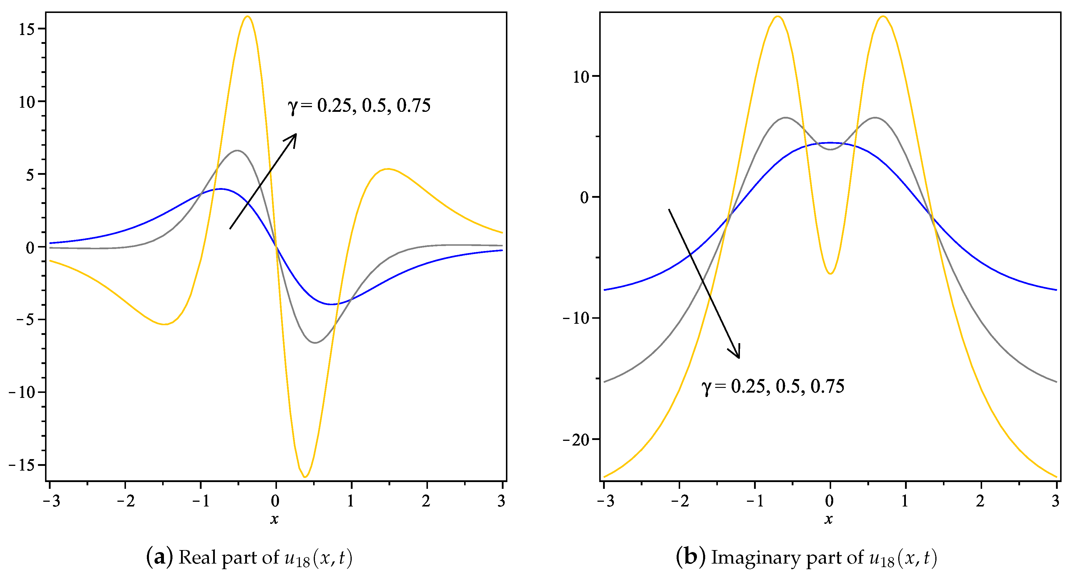
- For and in Equation (1), the unknown coefficients are given by,Therefore, the exact complex solution of Equation (1) is given by,The 2D graphs of real and imaginary parts of are drawn in Figure 11.Further, for the same and value, the second set of unknown coefficients are given by,
4. Conclusions
In this work, the generalized Kuramoto–Sivashinsky equation is solved, and the exact solutions have been found. The aforesaid GKSE has solutions for the different values of and , which we obtained by the application of the modified Kudryashov method, and we found 10 classes of pairs and their corresponding two distinct exact solutions for each pair of Equation (1) in Cases 1–10. The two-dimensional simulations of the solutions in Figure 1, Figure 2, Figure 3, Figure 4, Figure 5, Figure 6, Figure 7, Figure 8, Figure 9, Figure 10, Figure 11 and Figure 12 show their behavioral pattern and wave train traveling for different values of . However, the wave structures vary when the values of and the domain changes in the 2D plane. The solutions found in this work will be useful in studying electromagnetic waves, fluid flows and the areas where GKSE plays a vital role. All the solutions are validated in the Maple computer algebra system by substituting them in the original equation. Our new solutions are compared with the previous solutions of GKSE in Appendix A and Appendix B.
Author Contributions
Both authors contributed equally. Both authors read and approved the final manuscript.
Funding
The research is partially supported by the University Putra Malaysia research grant having vot number UPM-GPB/2017/9543000.
Conflicts of Interest
The authors declare no conflict of interest.
Appendix A. GKSE in the Previous Studies
N.A. Kudryashov in [6] solved for the exact solution of Equation (1). Based on the homogeneous balancing, he has taken the following initial solution.
where is the solution of , and obtained the following values.
In the same work, he solved Equation (1) with the auxiliary equations and and obtained other values for unknowns.
C.M. Khalique in [9] solved Equation (1) by taking the Bernoulli equation and Riccati equation as the auxiliary ODE and obtained the following values respectively by using each ODE. For both the auxiliary equation the constant values are and :
While comparing the above values, our solutions of Equation (1) in this work are new to the surveyed literature.
Appendix B. Studying GKSE by GKM and SGEEM
- For solving Equation (1) by the generalized Kudryashov method [22,23,24], the homogeneous balancing of Equation (8) gives , which has infinite solutions. For the value , this gives . Therefore,where is the solution of , Applying these equations to Equation (8) leads to the polynomial in and its powers. Collecting the coefficients of and attempting to solve the overdetermined equations results in the continuous execution of Maple. Hence, we conclude that Equation (1) cannot be solved by the generalized Kudryashov method.
- Next, for solving Equation (1) by the sine-Gordon equation expansion method [26], the homogeneous balancing is the same as the MKM given by . Thus,Substituting the above equation in Equation (8) and following the steps in [26] lead to the polynomials in , , their products and powers. Collecting the coefficients, equating them to zero and solving in Maple result in the continuous execution. Thus, we conclude that Equation (1) cannot be solved by the sine-Gordon equation expansion method either.
References
- Kudryashov, N.A. Exact solutions of the generalized Kuramoto-Sivashinsky equation. Phys. Lett. A 1990, 147, 287–290. [Google Scholar] [CrossRef]
- Parkes, E.J.; Duffy, B.R. An automated tanh-function method for finding solitary wave solutions to non-linear evolution equations. Comput. Phys. Commun. 1996, 98, 288–300. [Google Scholar] [CrossRef]
- Hamid, B.A. An exact solution to the Kuramoto-Sivashinsky equation. Phys. Lett. A 1999, 263, 338–340. [Google Scholar] [CrossRef]
- Baldwin, D.; Göktas, Ü.; Hereman, W.; Hong, L.; Martino, R.S.; Miller, J.C. Symbolic computation of exact solutions expressible in hyperbolic and elliptic functions for nonlinear PDEs. J. Symb. Comput. 2004, 37, 669–705. [Google Scholar] [CrossRef]
- Li, C.; Chen, G.; Zhao, S. Exact travelling wave solutions to the generalized Kuramoto-Sivashinsky equation. Latin Am. Appl. Res. 2004, 34, 65–68. [Google Scholar]
- Kudryashov, N.A. Solitary and Periodic Solutions of the Generalized Kuramoto-Sivashinsky Equation. Regul. Chaotic Dyn. 2008, 13, 234–238. [Google Scholar] [CrossRef]
- Khater, A.H.; Temsah, R.S. Numerical solutions of the generalized Kuramoto-Sivashinsky equation by Chebyshev spectral collocation methods. Comput. Math. Appl. 2008, 56, 1465–1472. [Google Scholar] [CrossRef]
- Porshokouhi, M.G.; Ghanbari, B. Application of He’s variational iteration method for solution of the family of Kuramoto-Sivashinsky equations. J. King Saud Univ.-Sci. 2011, 23, 407–411. [Google Scholar] [CrossRef]
- Khalique, C.M. Exact Solutions of the Generalized Kuramoto-Sivashinsky Equation. Caspian J. Math. Sci. 2012, 1, 109–116. [Google Scholar]
- Feng, D. Exact Solutions of Kuramoto-Sivashinsky Equation. Int. J. Educ. Manag. Eng. 2012, 6, 61–66. [Google Scholar] [CrossRef]
- Lakestani, M.; Dehghan, M. Numerical solutions of the generalized Kuramoto-Sivashinsky equation using B-spline functions. Appl. Math. Model. 2012, 36, 605–617. [Google Scholar] [CrossRef]
- Yang, J.; Lu, X.; Tang, X. Exact travelling wave solutions for the generalized Kuramoto-Sivashinsky equation. J. Math. Sci. Adv. Appl. 2015, 31, 1–13. [Google Scholar]
- Rashidinia, J.; Jokar, M. Polynomial scaling functions for numerical solution of generalized Kuramoto-Sivashinsky equation. Appl. Anal. 2015, 10, 1–10. [Google Scholar] [CrossRef]
- Acan, O.; Keskin, Y. Approximate solution of Kuramoto-Sivashinsky equation using reduced differential transform method. AIP Conf. Proc. 2015, 1648, 470003-1–470003-4. [Google Scholar]
- Foroutan, M.; Manafian, J.; Taghipour-Farshi, H. Exact solutions for Fitzhugh-Nagumo model of nerve excitation via Kudryashov method. Opt. Quantum Electron. 2017, 49, 352. [Google Scholar] [CrossRef]
- Ali, K.K.; Nuruddeen, R.I.; Hadhoud, A.R. New exact solitary wave solutions for the extended (3 + 1)-dimensional Jimbo-Miwa equations. Results Phys. 2018, 9, 12–16. [Google Scholar] [CrossRef]
- Hosseini, K.; Mayeli, P.; Ansari, R. Modified Kudryashov method for solving the conformable time-fractional Klein-Gordon equations with quadratic and cubic nonlinearities. Optik 2017, 130, 737–742. [Google Scholar] [CrossRef]
- Hosseini, K.; Ansari, R. New exact solutions of nonlinear conformable time-fractional Boussinesq equations using the modified Kudryashov method. Waves Random Complex Med. 2017, 27, 628–636. [Google Scholar] [CrossRef]
- Kumar, D.; Seadawy, A.R.; Joardar, A.K. Modified Kudryashov method via new exact solutions for some conformable fractional differential equations arising in mathematical biology. Chin. J. Phys. 2018, 56, 75–85. [Google Scholar] [CrossRef]
- Joardar, A.K.; Kumar, D.; al Woadud, K.M.A. New exact solutions of the combined and double combined sinh-cosh-Gordon equations via modified Kudryashov method. Int. J. Phys. Res. 2018, 1, 25–30. [Google Scholar] [CrossRef]
- Seadawy, A.R.; Kumar, D.; Hosseini, K.; Samadani, F. The system of equations for the ion sound and Langmuir waves and its new exact solutions. Results Phys. 2018, 9, 1631–1634. [Google Scholar]
- Mahmud, F.; Samsuzzoha, M.; Akbar, M.A. The generalized Kudryashov method to obtain exact traveling wave solutions of the PHI-four equation and the Fisher equation. Results Phys. 2017, 7, 4296–4302. [Google Scholar] [CrossRef]
- Demiray, S.T.; Pandir, Y.; Bulut, H. Generalized Kudryashov Method for Time-Fractional Differential Equations. Abstract Appl. Anal. 2014, 2014, 901540. [Google Scholar]
- Bibi, S.; Ahmed, N.; Khan, U.; Mohyud-Din, S.T. Some new exact solitary wave solutions of the van der Waals model arising in nature. Results Phys. 2018, 9, 648–655. [Google Scholar] [CrossRef]
- Raslan, K.R.; L-Danaf, T.S.E.; Ali, K.K. New exact solutions of coupled generalized regularized long wave equations. J. Egypt. Math. Soc. 2017, 25, 400–405. [Google Scholar] [CrossRef]
- Bulut, H.; Sulaiman, T.A.; Baskonus, H.M.; Sandulyak, A.A. New solitary and optical wave structures to the (1 + 1)-dimensional combined KdV-mKdV equation. Optik 2017, 135, 327–336. [Google Scholar] [CrossRef]
- Baskonus, H.M.; Sulaiman, T.A.; Bulut, H. Dark, bright and other optical solitons to the decoupled nonlinear Schrödinger equation arising in dual-core optical fibers. Opt. Quantum Electron. 2018, 50, 165. [Google Scholar] [CrossRef]
- Yang, X.-L.; Tang, J.-S. Travelling Wave Solutions for Konopelchenko-Dubrovsky Equation Using an Extended sinh-Gordon Equation Expansion Method. Commun. Theor. Phys. 2008, 50, 1047–1051. [Google Scholar]
- Esen, A.; Sulaiman, T.A.; Bulut, H.; Baskonus, H.M. Optical solitons to the space-time fractional (1+1)-dimensional coupled nonlinear Schrödinger equation. Optik 2018, 167, 150–156. [Google Scholar] [CrossRef]
- Gepreel, K.A. Extended trial equation method for nonlinear coupled Schrodinger Boussinesq partial differential equations. J. Egypt. Math. Soc. 2016, 24, 381–391. [Google Scholar] [CrossRef]
- Pandir, Y.; Gurefe, Y.; Misirli, E. The Extended Trial Equation Method for Some Time Fractional Differential Equations. Discret. Dyn. Nat. Soc. 2013, 2013, 491359. [Google Scholar] [CrossRef]
- Gurefe, Y.; Misirli, E.; Sonmezoglu, A.; Ekici, M. Extended trial equation method to generalized nonlinear partial differential equations. Appl. Math. Comput. 2013, 219, 5253–5260. [Google Scholar] [CrossRef]
- Ravi, L.K.; Ray, S.S.; Sahoo, S. New exact solutions of coupled Boussinesq-Burgers equations by Exp-function method. J. Ocean Eng. Sci. 2017, 2, 34–46. [Google Scholar] [CrossRef]
- Seadawy, A.R.; Lu, D.; Khater, M.M.A. Solitary wave solutions for the generalized Zakharov-Kuznetsov-Benjamin-Bona-Mahony nonlinear evolution equation. J. Ocean Eng. Sci. 2017, 2, 137–142. [Google Scholar] [CrossRef]
- Alam, M.N.; Alam, M.M. An analytical method for solving exact solutions of a nonlinear evolution equation describing the dynamics of ionic currents along microtubules. J. Taibah Univ. Sci. 2017, 11, 939–948. [Google Scholar] [CrossRef]
- Liu, S.; Fu, Z.; Liu, S.; Zhao, Q. Jacobi elliptic function expansion method and periodic wave solutions of nonlinear wave equations. Phys. Lett. A 2001, 289, 69–74. [Google Scholar] [CrossRef]
- Ebaid, A.; Aly, E.H. Exact solutions for the transformed reduced Ostrovsky equation via the F-expansion method in terms of Weierstrass-elliptic and Jacobian-elliptic functions. Wave Motion 2012, 49, 296–308. [Google Scholar] [CrossRef]
- Zayed, E.M.E.; Al-Joudi, S. Applications of an Extended G′/G-Expansion Method to Find Exact Solutions of Nonlinear PDEs in Mathematical Physics. Math. Probl. Eng. 2010, 2010, 768573. [Google Scholar] [CrossRef]
Figure 1.
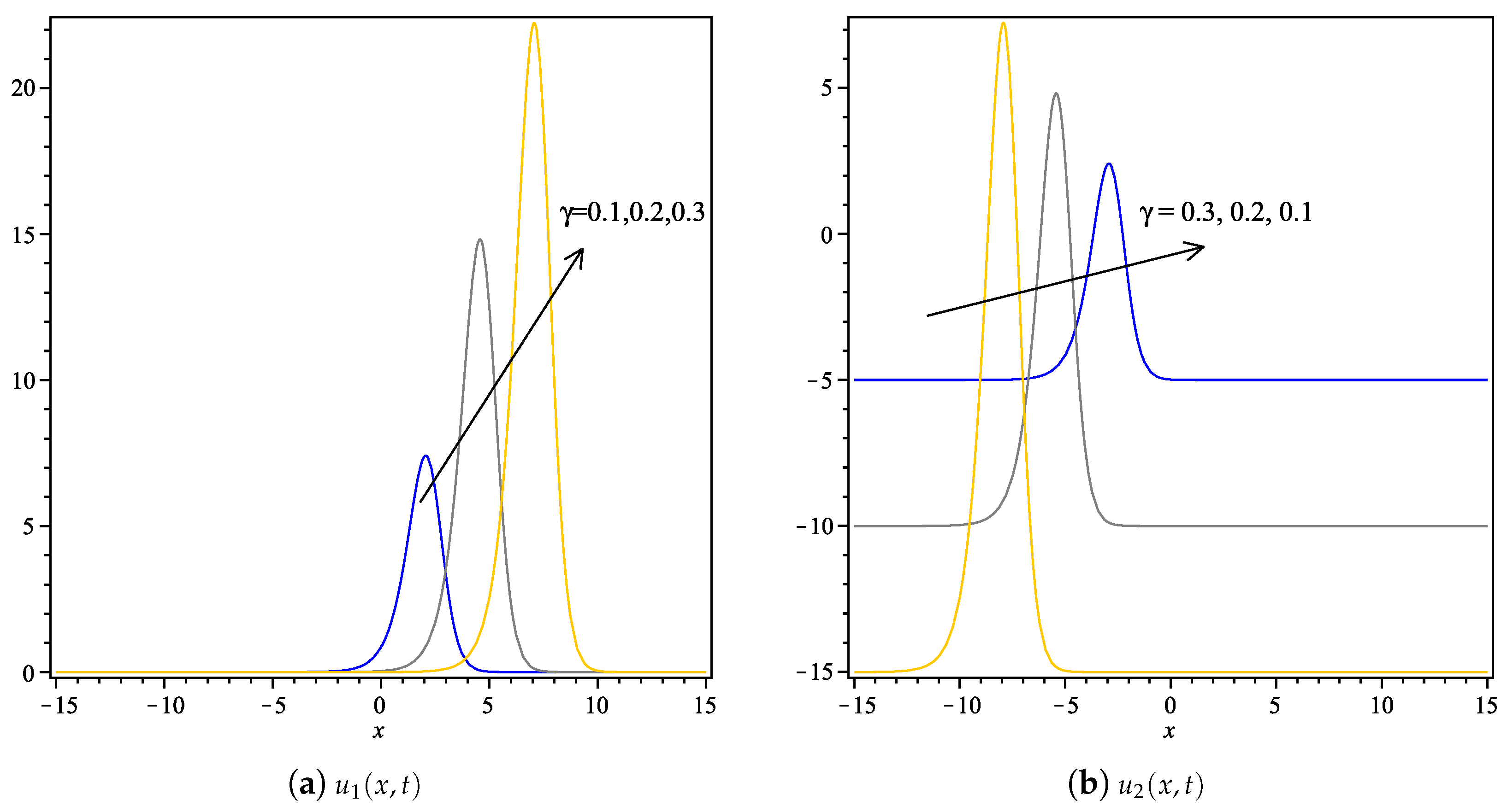
Solutions in Case 1, Equations (10) and (11), respectively from left to right for a = 5, μ = 1 and t = 1 in x ∈ [−15, 15] for different values of γ.
Figure 1.
Solutions in Case 1, Equations (10) and (11), respectively from left to right for a = 5, μ = 1 and t = 1 in x ∈ [−15, 15] for different values of γ.

Figure 2.
Solutions in Case 2, Equations (12) and (13), respectively from left to right for a = 5, μ = 1 and t = 1 in x ∈ [−15, 15] for different values of γ.
Figure 2.
Solutions in Case 2, Equations (12) and (13), respectively from left to right for a = 5, μ = 1 and t = 1 in x ∈ [−15, 15] for different values of γ.

Figure 3.
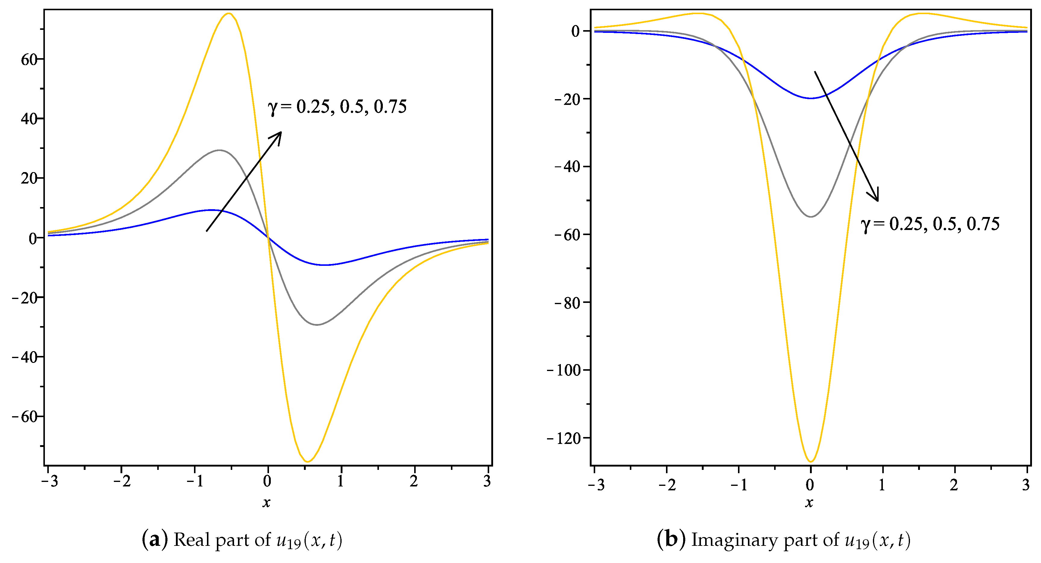
Solutions in Case 3, Equations (14) and (15), respectively from left to right for a = 5, μ = 1 and t = 1 in x ∈ [−40, 40] for u5(x, t) and in x ∈ [−50, 50] for u6(x, t) for different values of γ.
Figure 3.
Solutions in Case 3, Equations (14) and (15), respectively from left to right for a = 5, μ = 1 and t = 1 in x ∈ [−40, 40] for u5(x, t) and in x ∈ [−50, 50] for u6(x, t) for different values of γ.
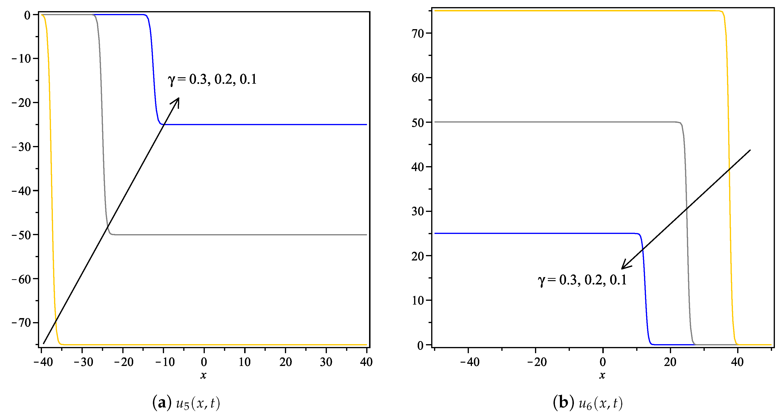
Figure 4.
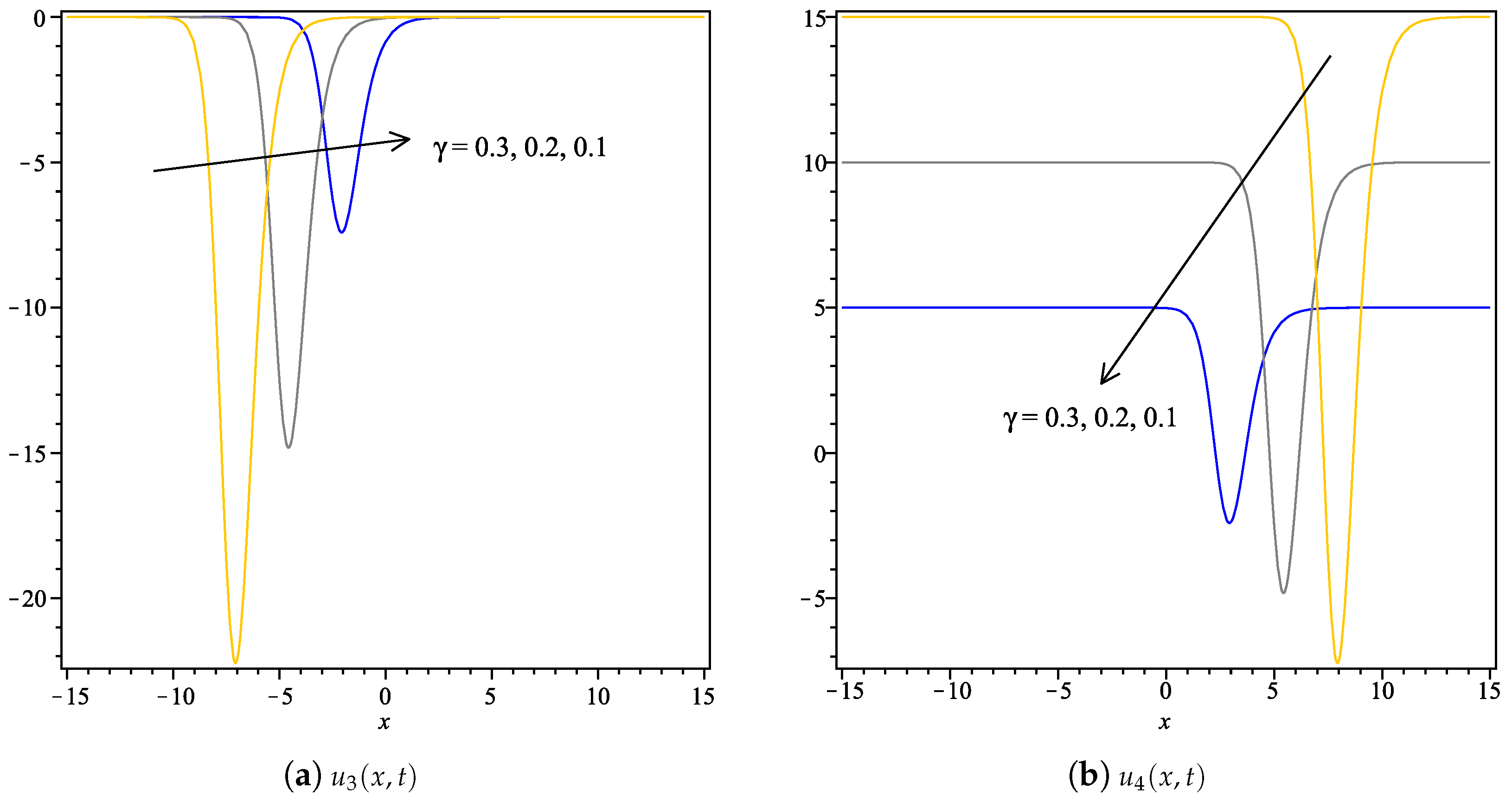
Solutions in Case 4, Equations (16) and (17), respectively from left to right for a = 5, μ = 1 and t = 1 in x ∈ [−15, 15] for different values of γ.
Figure 4.
Solutions in Case 4, Equations (16) and (17), respectively from left to right for a = 5, μ = 1 and t = 1 in x ∈ [−15, 15] for different values of γ.

Figure 5.
Solutions in Case 5, Equations (18) and (19), respectively from left to right for a = 5, μ = 1 and t = 1 in x ∈ [−15, 15] for different values of γ.
Figure 5.
Solutions in Case 5, Equations (18) and (19), respectively from left to right for a = 5, μ = 1 and t = 1 in x ∈ [−15, 15] for different values of γ.
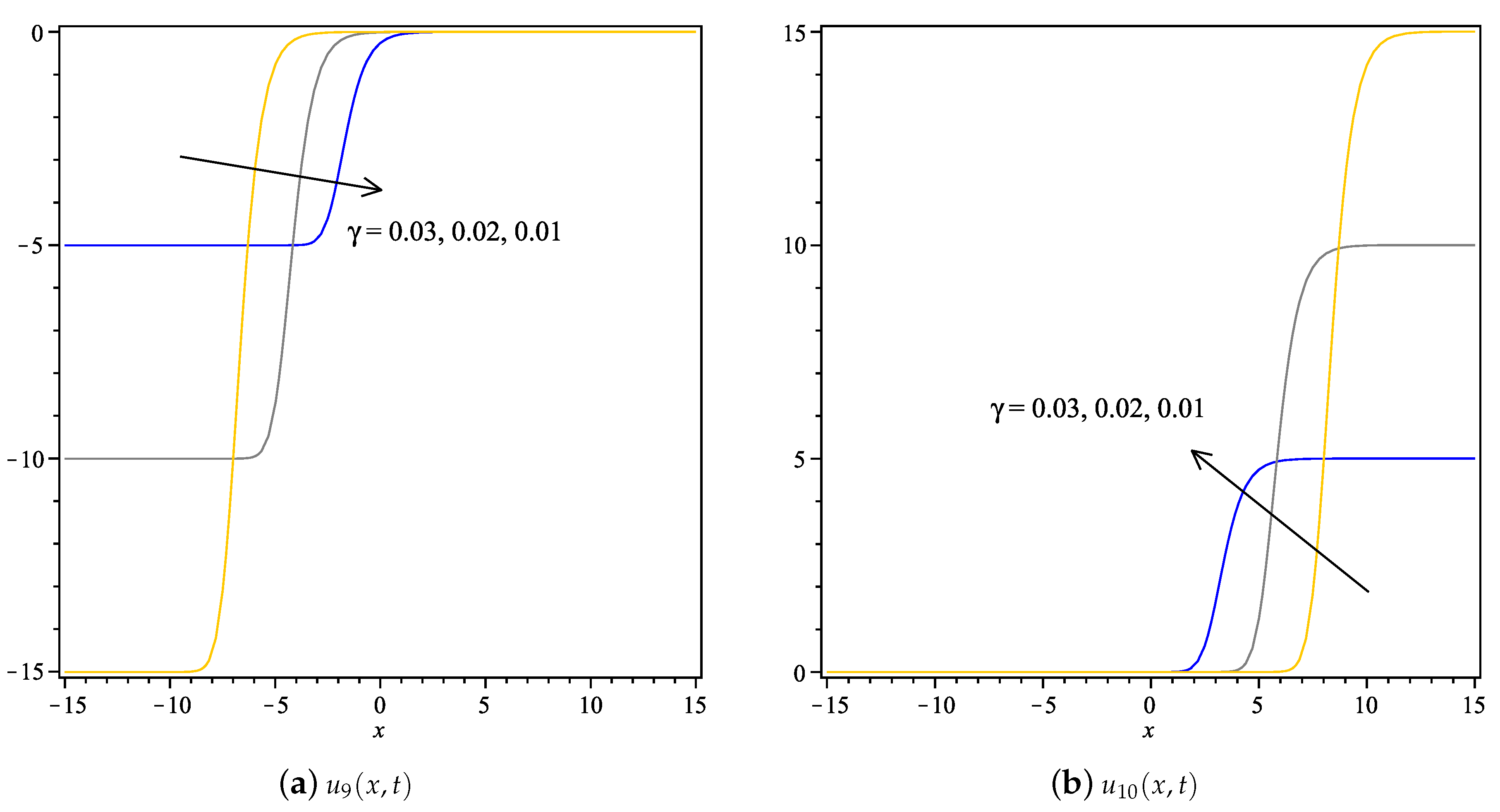
Figure 6.
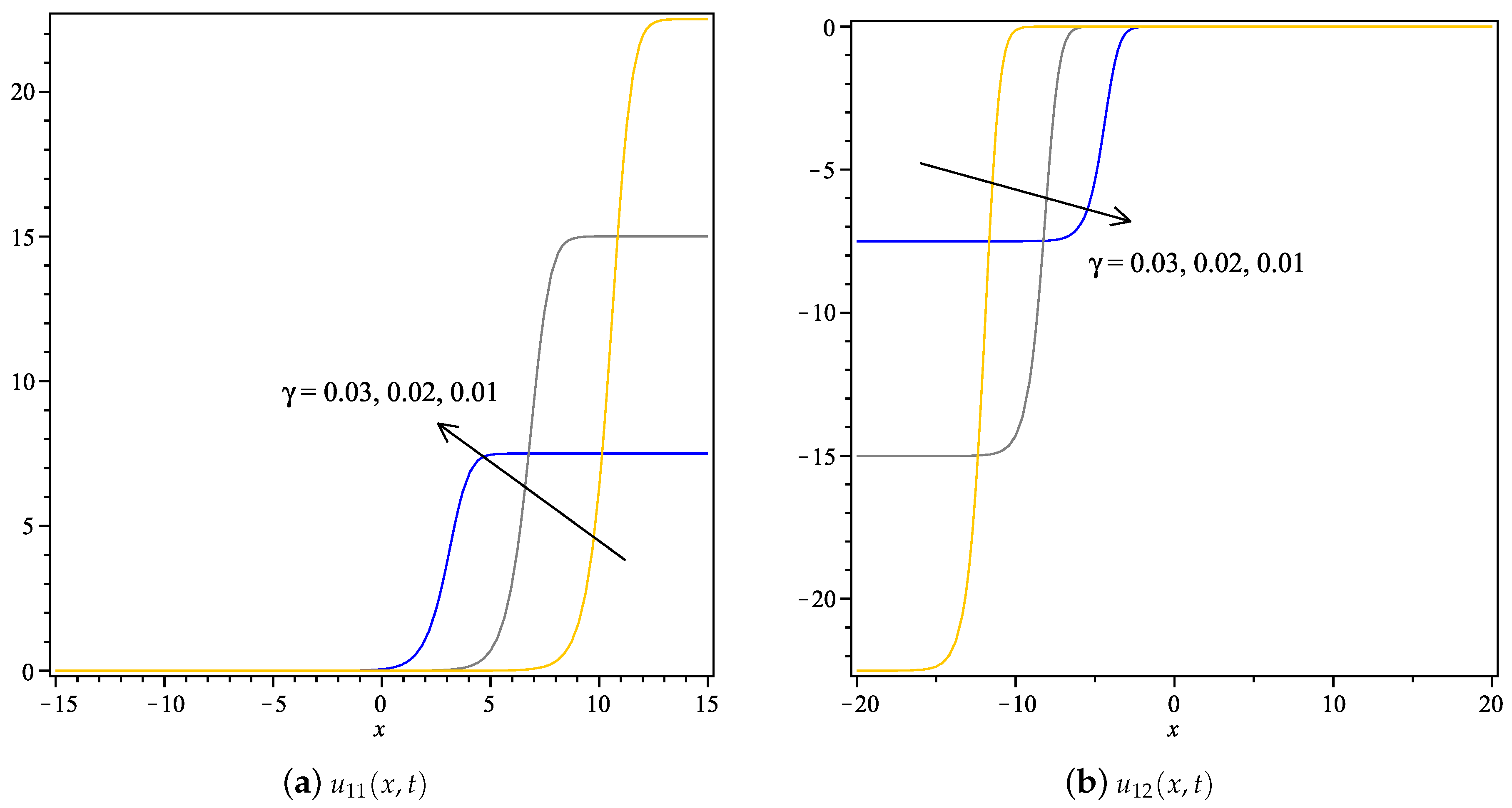
Solutions in Case 6, Equations (20) and (21), respectively from left to right for a = 5, μ = 1 and t = 1 in x ∈ [−15, 15] for u11(x, t) and x ∈ [−20, 20] for u12(x, t) for different values of γ.
Figure 6.
Solutions in Case 6, Equations (20) and (21), respectively from left to right for a = 5, μ = 1 and t = 1 in x ∈ [−15, 15] for u11(x, t) and x ∈ [−20, 20] for u12(x, t) for different values of γ.

Figure 7.
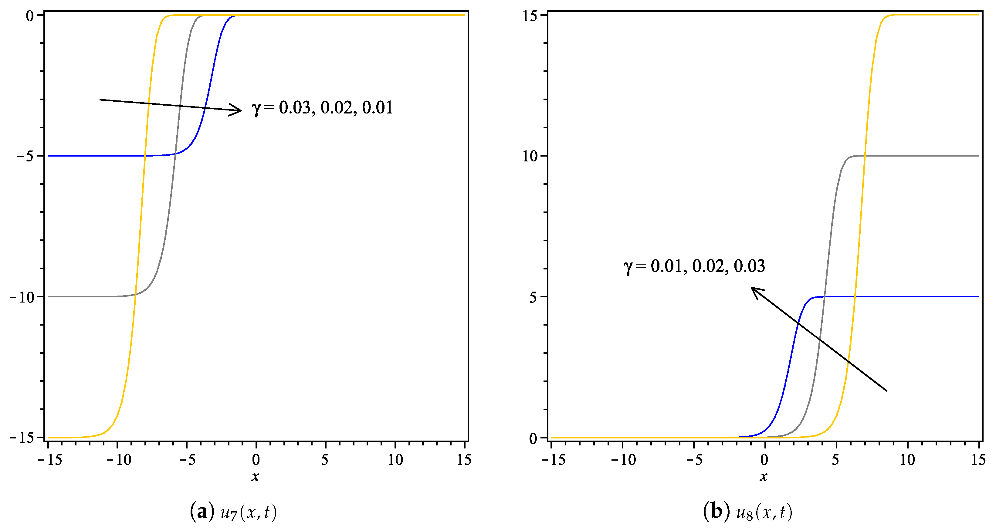
Solutions in Case 7, Equations (22) and (23), respectively from left to right for a = 5, μ = 1 and t = 1 in x ∈ [−20, 20] for different values of γ.
Figure 7.
Solutions in Case 7, Equations (22) and (23), respectively from left to right for a = 5, μ = 1 and t = 1 in x ∈ [−20, 20] for different values of γ.
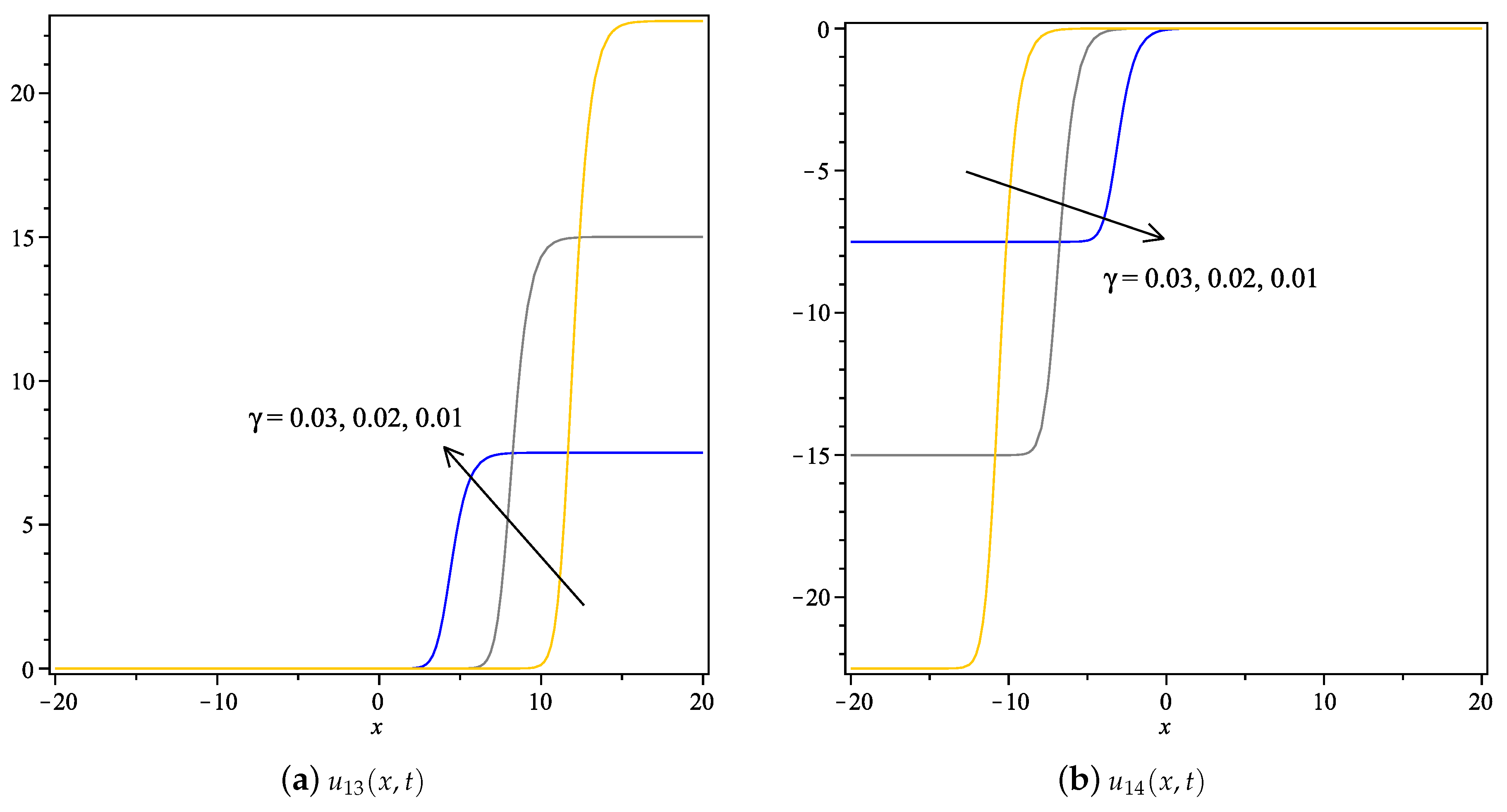
Figure 8.
Solutions in Case 8, Equations (24) and (25), respectively from left to right for a = 5, μ = 1 and t = 1 in x ∈ [−20, 20] for different values of γ.
Figure 8.
Solutions in Case 8, Equations (24) and (25), respectively from left to right for a = 5, μ = 1 and t = 1 in x ∈ [−20, 20] for different values of γ.
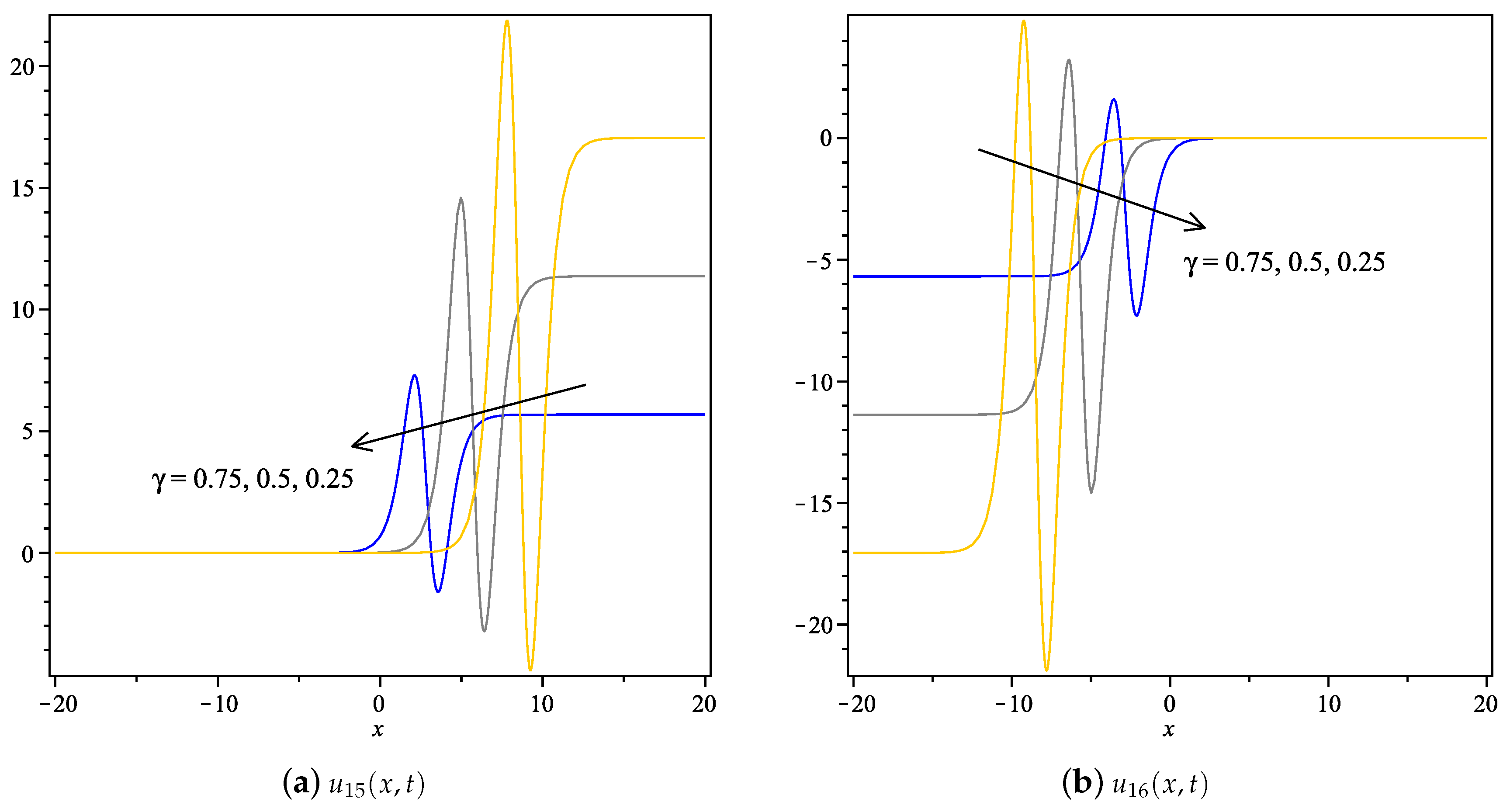
Figure 9.
Real and imaginary part of the solution in Case 9, Equation (26), respectively from left to right for a = 5, μ = 1 and t = 1 in x ∈ [−3, 3] for different values of γ.
Figure 9.
Real and imaginary part of the solution in Case 9, Equation (26), respectively from left to right for a = 5, μ = 1 and t = 1 in x ∈ [−3, 3] for different values of γ.
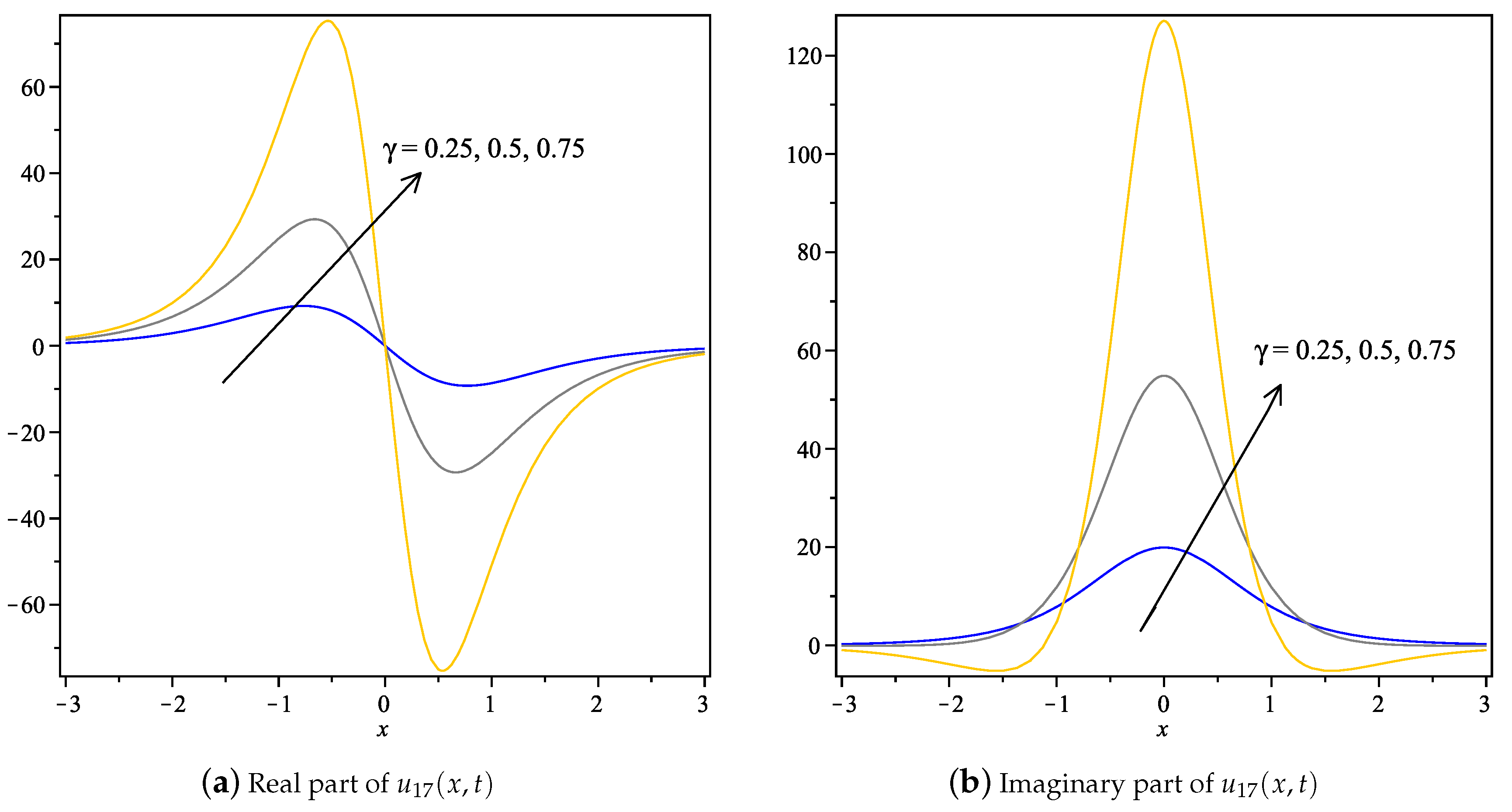
Figure 10.
Real and imaginary part of the solution in Case 9, Equation (27), respectively from left to right for a = 5, μ = 1 and t = 1 in x ∈ [−3, 3] for different values of γ.
Figure 10.
Real and imaginary part of the solution in Case 9, Equation (27), respectively from left to right for a = 5, μ = 1 and t = 1 in x ∈ [−3, 3] for different values of γ.

Figure 11.
Real and imaginary part of the solution in Case 10, Equation (28), respectively from left to right for a = 5, μ = 1 and t = 1 in x ∈ [−3, 3] for different values of γ.
Figure 11.
Real and imaginary part of the solution in Case 10, Equation (28), respectively from left to right for a = 5, μ = 1 and t = 1 in x ∈ [−3, 3] for different values of γ.

Figure 12.
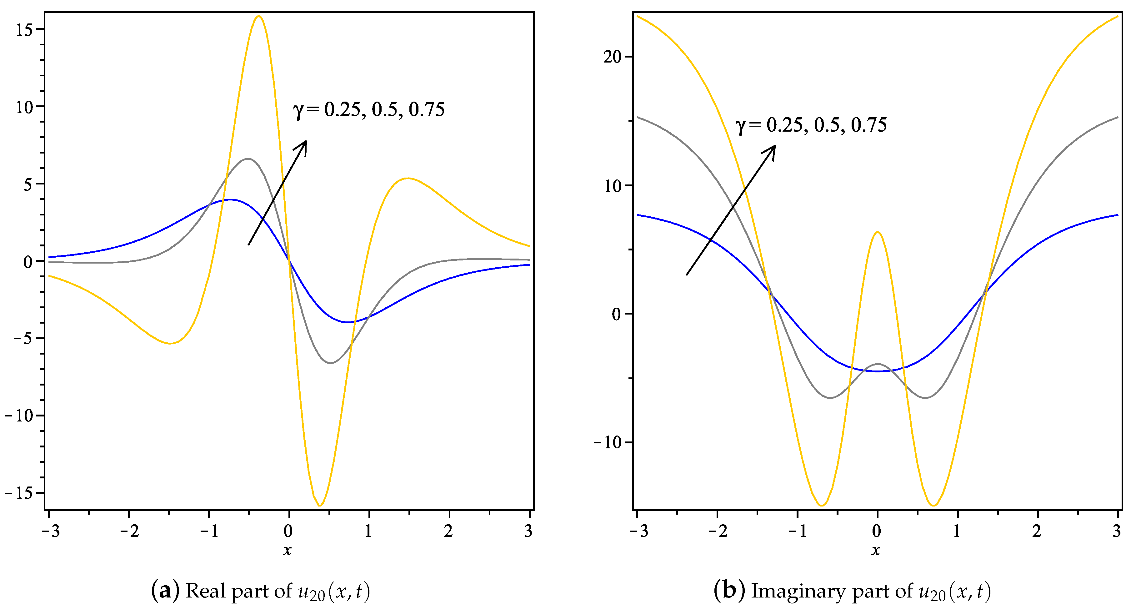
Real and imaginary part of the solution in Case 10, Equation (29), respectively from left to right for a = 7, μ = 1 and t = 1 in x ∈ [−3, 3] for different values of γ.
Figure 12.
Real and imaginary part of the solution in Case 10, Equation (29), respectively from left to right for a = 7, μ = 1 and t = 1 in x ∈ [−3, 3] for different values of γ.

© 2018 by the authors. Licensee MDPI, Basel, Switzerland. This article is an open access article distributed under the terms and conditions of the Creative Commons Attribution (CC BY) license (http://creativecommons.org/licenses/by/4.0/).
Share and Cite
MDPI and ACS Style
Kilicman, A.; Silambarasan, R. Modified Kudryashov Method to Solve Generalized Kuramoto-Sivashinsky Equation. Symmetry 2018, 10, 527. https://doi.org/10.3390/sym10100527
AMA Style
Kilicman A, Silambarasan R. Modified Kudryashov Method to Solve Generalized Kuramoto-Sivashinsky Equation. Symmetry. 2018; 10(10):527. https://doi.org/10.3390/sym10100527
Chicago/Turabian StyleKilicman, Adem, and Rathinavel Silambarasan. 2018. "Modified Kudryashov Method to Solve Generalized Kuramoto-Sivashinsky Equation" Symmetry 10, no. 10: 527. https://doi.org/10.3390/sym10100527
Note that from the first issue of 2016, this journal uses article numbers instead of page numbers. See further details here.