Underdetermined Blind Source Separation Combining Tensor Decomposition and Nonnegative Matrix Factorization

Abstract

Underdetermined blind source separation (UBSS) is a hot topic in signal processing, which aims at recovering the source signals from a number of observed mixtures without knowing the mixing system. Recently, expectation-maximization algorithm shows a great potential in the UBSS. However, the final separation results depend strongly on the parameter initialization, leading to poor separation performance. In this paper, we propose an effective algorithm that combines tensor decomposition and nonnegative matrix factorization (NMF). In the proposed algorithm, we first employ tensor decomposition to estimate the mixing matrix, and NMF source model is used to estimate the source spectrogram factors. Then a series of iterations are derived to update the model parameters. At the same time, the spatial images of source signals are estimated with Wiener filters constructed from the learned parameters. Therefore, time-domain sources can be obtained through inverse short-time Fourier transform. Finally, plenty of experimental results demonstrate the effectiveness and advantages of our proposed algorithm over the compared algorithms.

1. Introduction

Blind source separation (BSS) considers the recovery of source signals from observed signals without knowing the recording environment. Recently, the use of BSS has become an active research area. If the number of source signals is less, equal or greater than the number of microphones, BSS can be classified as the overdetermined case [1], the determined case [2,3], or the underdetermined case [4,5], respectively. In particular, in the natural environment, the mixing process is generally considered to be convolutive, i.e., the channel between each source and each microphone is modeled in a linear filter that represents multiple source-to-microphone paths because it considers the reverberation of the channel. Therefore, underdetermined convolutive BSS is a challenging problem in the field of BSS.

To address this underdetermined convolutive BSS problem, tensor decomposition shows great potential, because an interesting property of higher-order tensors is that their rank decomposition is unique. Additionally, parallel factor (PARAFAC) decomposition factorizes a tensor into a sum of component rank-one tensors, and the factor matrices refer to the combination of the vectors from the rank-one components. By singular value decomposition of a series of matrices, the parallel factorization problem is transformed into a joint matrix diagonalization problem, such that the PARAFAC analysis is solved [6,7]. Therefore, the PARAFAC method can be used to identify the mixing matrix in the underdetermined case, which has been proven usefully in a wide range of applications from sensor array processing to communication, speech and audio signal processing [8,9]. In the phase of source separation, source signals can be estimated by using the $l_0$-norm minimization method [10] or the binary masking algorithm [11]. However, these methods suffer from poor separation performance. To improve separation performance, we found out that the source model includes some specific information on the spectral structures of sources. Therefore, a better source model has the potential to improve the source separation performance.

In BSS, the non-negative matrix factorization (NMF) source model is usually applied on the speech/music power spectrogram, where the spectrogram is approximated by the product of two non-negative matrices, i.e., a basis matrix and an activation matrix. The basis matrix represents the repeating spectral patterns, and the activation matrix represents the presence of these patterns over time. Additionally, NMF aims to decompose a non-negative factor matrix into the product of two low-rank non-negative factor matrices [12,13]. The NMF model can be used to efficiently exploit the low-rank nature of the speech spectrogram and its dependency across the frequencies. In some NMF-based methods [14,15,16,17], non-negative matrix factor two-dimensional deconvolution is an effective machine learning method in audio source separation field. In particular, in the convolutive frequency-domain model, the well-known permutation alignment problem cannot be solved without using additional a priori knowledge about the sources or the mixing filters. However, the NMF source model implies a coupling of the frequency bands, and joint estimation of the source parameters and mixing coefficients, which frees us from the permutation problem. Furthermore, NMF is well suited to polyphony as it basically takes the source to be a sum of elementary components with characteristic spectral signatures. Therefore, NMF source model is able to improve the source separation performance.

Additionally, in order to obtain better source separation results, the estimated mixing matrix and NMF variables need to be updated using an optimization algorithm. In most BSS optimization algorithms, we found out that expectation-maximization (EM) algorithm [18], which is a popular choice for Gaussian models, provided faster convergence. The EM algorithm is related to some multichannel source separation techniques by employing Gaussian mixture model as source models. However, it is very sensitive to initialization in source separation tasks. There had been some studies of parameter initialization of NMF to optimize separation performance [19,20]. Therefore, we try to take an optimization algorithm to improve the source separation performance.

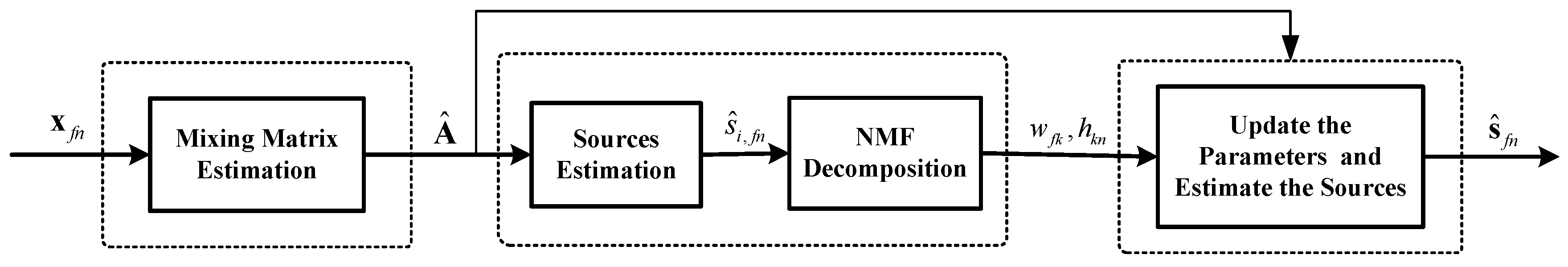
In this paper, an alternative optimization algorithm is proposed to deal with the parameter initialization problem and improve separation performance. First, we employ tensor decomposition to detect the mixing matrix, and NMF is used to estimate the source spectrogram factors. Then these model parameters are updated using the EM algorithm. Meanwhile, the spatial images of source signals are estimated using Wiener filters constructed from the learned parameters. The time-domain sources can be obtained through inverse short-term Fourier transform (STFT) using an adequate overlap-add procedure with dual synthesis window. Thanks to the linearity of the inverse STFT, the reconstruction is conservation in the time-domain as well. Finally, a series of experimental results including synthetic instantaneous and convolutive music and speech source mixtures, as well as live real recordings, show that our improved algorithm outperforms the state-of-the-art baseline methods. We can highlight the main contributions of this article as follows.

(1) We propose an improved algorithm that combines tensor decomposition and advanced NMF to deal with the underdetermined linear BSS. The mixing matrix is estimated using tensor decomposition, and NMF is used to decompose the given spectrogram into several spectral bases and temporal activations. Then the mixing matrix, NMF variables, and noise components are updated by a series of iteration rules. The proposed algorithm combines the advantages of tensor decomposition and NMF, which is beneficial to improve the performance of source separation. Additionally, the improved algorithm can be extended to underdetermined convolutive BSS.

(2) We have demonstrated the superiority in the underdetermined linear and convolutive BSS cases. Additionally, in this paper we mainly consider the audio datasets, the proposed algorithm demonstrates the effectiveness and superiority compared with the state-of-the-art algorithms, which improves the source separation performance based on a series of simulation experiments.

The structure of the remaining of this paper is organized as follows. Section 2 formulates the problem of the underdetermined blind source separation. In Section 3, an optimization algorithm is presented based on tensor decomposition and NMF. Experimental results compared the source separation performance with the state-of-the-art techniques in various experimental settings are shown in Section 4. Finally, Section 5 summarizes our conclusion and the future work.

2. Problem Formulation

2.1. Linear Instantaneous Mixture Model

The signal model with noise used in this paper is described as follows:

$$\mathbf{x}(t)=\mathbf{As}(t)+\mathbf{v}(t)$$

(1)

in which $\mathbf{x}(t)=[{\mathbf{x}}_1(t),\dots ,{\mathbf{x}}_J(t)]\in {\mathbb{C}}^J$ represents the received J signals, $\mathbf{s}(t)=[{\mathbf{s}}_1(t),\dots ,{\mathbf{s}}_I(t)]\in {\mathbb{C}}^I$ denotes the I source signals (unknown), and $I>J$, i.e., in the underdetermined mixture case. $\mathbf{A}=[{\mathbf{a}}_1,\dots ,{\mathbf{a}}_I]\in {\mathbb{C}}^{J\times I}$ is the unknown mixing matrix, $\mathbf{v}(t)\in {\mathbb{C}}^J$ is an additional noise with zero mean and variance ${\sigma }^2$.

Nevertheless, for audio signals, the separation is much easier in the short-time discrete frequency transform domain, where the source signals are sparser. Therefore, the mixture model (1) can be expressed as follows:

$${\mathbf{x}}_{fn}\approx {\mathbf{As}}_{fn}+{\mathbf{v}}_{fn}$$

(2)

where $n=1,2,\dots ,N$ denotes the index of the time window for applying the Fourier transform, $f=0,\dots ,F-1$ is the index of the frequency bins, ${\mathbf{x}}_{fn}={[x_{1,fn},\dots ,x_{J,fn}]}^T$ and ${\mathbf{s}}_{fn}={[s_{1,fn},\dots ,s_{I,fn}]}^T$ are the STFT of the mixtures and the sources at time-frequency point $(f,n)$, respectively. ${\mathbf{v}}_{fn}={[v_{1,fn},\dots ,v_{J,fn}]}^T$, the noise $v_{j,fn}$ is assumed to be stationary and spatially uncorrelated, i.e., $v_{j,fn}\sim {\mathbb{N}}_c(0,{\sigma }_{j,f}^2)$ and ${\Sigma }_{\mathbf{v},f}=diag[{\sigma }_{j,f}^2]$.

2.2. The NMF Source Model

Let $K\ge I$ is known in advance, and ${\{{\mathcal{K}}_i\}}_{i=1}^I$ be a nontrivial partition of $\mathcal{K}=1,\dots ,K$. Following [16,17], a coefficient $s_{i,fn}$ is modeled as the sum of latent components $c_{k,fn}$, such that

$$s_{i,fn}=\sum _{k\in {\mathcal{K}}_i}{c}_{k,fn}\iff {\mathbf{s}}_{fn}={\mathbf{Gc}}_{fn}$$

(3)

where $\mathbf{G}\in {\mathbb{N}}^{I\times K}$ is a binary selection matrix with entries

$$G_{ik}=\{\begin{array}{c}1,k\in {\mathcal{K}}_i\hfill \\ 0,\mathrm{otherwise}\hfill \end{array}$$

and ${\mathbf{c}}_{fn}=[c_{1,fn},\dots ,c_{K,fn}]\in {\mathbb{C}}^K$ is the vector of component coefficients at $(f,n)$. Each component $c_{k,fn}$ follows that

$$c_{k,fn}\sim {\mathbb{N}}_c(0,w_{fk}{h}_{kn})$$

(4)

where ${\mathbb{N}}_c(\mu ,\Sigma )$ denotes the proper multivariate complex Gaussian distribution [21] with probability density function (pdf) ($N_c(\mathbf{x};\mu ,\Sigma )={|\pi \Sigma |}^{-1}\exp [-{(\mathbf{x}-\mu )}^H{\Sigma }^{-1}(\mathbf{x}-\mu )]$ is the proper complex Gaussian distribution.), $w_{fk},h_{kn}\in {\mathbb{R}}^{+}$, $w_{fk}$ represents the spectral basis of i-th source, and $h_{fk}$ represents the temporal code for each spectral basis element of the i-th source. In the rest of the paper, the quantities $s_{i,fn}$ and $c_{k,fn}$ are referred to as “source" and “component", respectively. The components are assumed to be mutually independent and individually independent across frequency and time. It follows that

$$s_{i,fn}\sim {\mathbb{N}}_c(0,\sum _{k\in {\mathcal{K}}_i}{w}_{fk}{h}_{kn})$$

(5)

This corresponds to model the source power spectral densities (PSD) with the NMF model, i.e.,

$$E[|{\mathbf{S}}_i{|}^2]={\mathbf{W}}_i{\mathbf{H}}_i$$

(6)

where ${\mathbf{S}}_i$ denotes the $F\times N$ STFT matrix of source i and the matrices ${\mathbf{W}}_i={[w_{fk}]}_{f,k\in {\mathcal{K}}_i}$, ${\mathbf{H}}_i={[h_{kn}]}_{k\in {\mathcal{K}}_i,n}$, respectively. Then for the maximum likelihood estimation of ${\mathbf{W}}_i$ and ${\mathbf{H}}_i$, it is shown that the minus log-likelihood (ML) of the parameters describing ${\mathbf{S}}_i$ writes

$$-logp({\mathbf{S}}_i|{\mathbf{W}}_i,{\mathbf{H}}_i)=\sum _{fn}{d}_{IS}(|s_{i,fn}{|}^2|\sum _{k\in {\mathcal{K}}_i}{w}_{fk}{h}_{kn})+\mathit{cst}$$

(7)

where “cst” denotes constant terms and

$$d_{IS}(x|y)=\frac{x}{y}-log\frac{x}{y}-1$$

(8)

is the Itakura-Satio (IS) Divergence (In this paper, the Itakura-Satio divergence is chosen as a measure of fit, which is appropriate for Gamma multiplicative noise. In addition, the Euclidean distance can cope with Gaussian additive noise and the Kullback-Leibler divergence fits multinomial distributions or Poisson noise.).

In addition, the following two types of divergence are widely used [20]:

Squared Euclidean (EU) distance

$$d_{EU}(x|y)={|x-y|}^2$$

(9)

Kullback-Leibler(KL) divergence

$$d_{KL}(x|y)=x·log\frac{x}{y}-x+y$$

(10)

Therefore, the ML estimation of ${\mathbf{W}}_i$ and ${\mathbf{H}}_i$ given source STFT ${\mathbf{S}}_i$ is equivalent to NMF of the power spectrogram $|{\mathbf{S}}_i{|}^2$ into ${\mathbf{W}}_i{\mathbf{H}}_i$. In our simulation experiments, we build the initialization of the source spectrogram estimation using the EU divergence, KL divergence, and IS divergence, respectively.

2.3. Objective

We are interested in jointly updating the source spectrogram factors ${\mathbf{W}}_i$, ${\mathbf{H}}_i$, the mixing matrix $\mathbf{A}$, and estimating the sources at the same time. In this paper, we propose a robust parameter initialization scheme to optimize EM algorithm. The block diagram of our proposed BSS algorithm is shown in Figure 1. Initially, tensor method is used to estimate the mixing matrix $\mathbf{A}$. Then the time-frequency sources are estimated and the source spectrogram factors are detected using NMF of the power spectrogram. Finally, the model parameters are updated and the spatial images of source signals are estimated. Detailed descriptions of each step are given in the following section.

3. The Proposed Optimization Algorithm

In the following, we will propose a robust parameters initialization scheme using tensor decomposition and NMF to optimize the EM algorithm. First, the mixing matrix is estimated using tensor decomposition. Second, the state-of-the-art source separation algorithms are reviewed. Finally, the optimization algorithm is presented in detail.

3.1. Mixing Matrix Estimation Using Tensor Decomposition

Let us denote the $J\times J$ auto-correlation matrix as follows:

$$\begin{array}{cc}\hfill {\mathbf{R}}_{\mathbf{x}}& =E[\mathbf{x}(t){\mathbf{x}}^H(t)]\hfill \\ & ={\mathbf{AR}}_{\mathbf{s}}{\mathbf{A}}^H\hfill \end{array}$$

(11)

where ${\mathbf{R}}_{\mathbf{s}}=E[{\mathbf{ss}}^H]$ is the auto-correlation matrix of the source signal, the superscripts ${·}^H$ denotes the complex conjugate transpose. For simplicity, we have dropped the noise terms. Let us divide the whole data block into P non-overlapping sub-blocks, which are indexed by $p=1,\dots ,P$. Then the spatial covariance matrices of the observation satisfy

$$\left\{\begin{array}{cc}{\mathbf{R}}_{\mathbf{x}}^1\hfill & =\mathbf{A}·{\mathbf{R}}_{\mathbf{s}}^1·{\mathbf{A}}^H\hfill \\ & ⋮\hfill \\ {\mathbf{R}}_{\mathbf{x}}^P\hfill & =\mathbf{A}·{\mathbf{R}}_{\mathbf{s}}^P·{\mathbf{A}}^H\hfill \end{array}\right.$$

(12)

in which ${\mathbf{R}}_{\mathbf{s}}^p=E[s_p{s}_p^H]$ is diagonal. The problem we want to solve is the estimation of $\mathbf{A}$ from the set ${\mathbf{R}}_{\mathbf{x}}^p$. The solution will be obtained by interpreting as a tensor decomposition. It can equivalently be written as PARAFAC decomposition of a third-order tensor ${\mathcal{R}}_{\mathbf{x}}\in {\mathbb{C}}^{J\times J\times P}$ built by stacking the P matrices $\{{\mathbf{R}}_{\mathbf{x}}^1,\dots ,{\mathbf{R}}_{\mathbf{x}}^P\}$ one after each other along the third dimension. Each element of the tensor ${\mathcal{R}}_{\mathbf{x}}$ is denoted by $r_{j_1,j_2,p}^{(x)}$, with $j_1=1,\dots ,J$, $j_1=1,\dots ,J$, and $p=1,\dots ,P$. Define the matrix $\mathbf{C}\in {\mathbb{C}}^{P\times I}$ whose element on the p-th row and i-th column, denoted $c_{p,i}$, is the i-th diagonal element of ${\mathbf{R}}_{\mathbf{s}}$. Then we have

$$r_{j_1,j_2,p}^{(x)}=\sum _{i=1}^I{a}_{j_1,i}{c}_{p,i}{a}_{j_{2}i}^{*}$$

(13)

The PARAFAC decomposition (13) of the tensor ${\mathcal{R}}_{\mathbf{x}}\in {\mathbb{C}}^{J\times J\times P}$ is a decomposition ${\mathcal{R}}_{\mathbf{x}}$ as a linear combination of a minimal number of rank-1 term:

$${\mathcal{R}}_{\mathbf{x}}=\sum _{i=1}^I{\mathbf{a}}_i\circ {\mathbf{c}}_i\circ {\mathbf{a}}_i^{*}$$

(14)

where ∘ denotes the tensor outer product, the superscripts ${·}^{*}$ denotes the complex conjugate, ${\mathbf{a}}_i$ and ${\mathbf{c}}_i$ are the column of $\mathbf{A}$ and $\mathbf{C}$, respectively.

In this paper, we will use the following $J^2\times P$ matrix representation of ${\mathcal{R}}_{\mathbf{x}}$ [22,23]

$${[{\mathbf{R}}_{\mathbf{x}}]}_{(j_1-1)J+j_2,p}={[{\mathcal{R}}_{\mathbf{x}}]}_{j_1,j_2,p}$$

(15)

Then (14) can be written in a matrix format as

$${\mathbf{R}}_{\mathbf{x}}=[\mathbf{A}\odot {\mathbf{A}}^{*}]·{\mathbf{C}}^T$$

(16)

where ⊙ denotes the Khatri-Rao product. As a result, its reduced-size SVD can be written as

$${\mathbf{R}}_{\mathbf{x}}=\mathbf{U}\mathbf{\Sigma }{\mathbf{V}}^H$$

(17)

where $\mathbf{U}\in {\mathbb{C}}^{J^2\times I}$, $\mathbf{\Sigma }\in {\mathbb{R}}^{I\times I}$ is diagonal, and $\mathbf{V}\in {\mathbb{C}}^{P\times I}$. Then there exists a nonsingular matrix $\mathbf{Z}\in {\mathbb{C}}^{I\times I}$, such that

$$\left\{\begin{array}{cc}\mathbf{A}\odot {\mathbf{A}}^{*}\hfill & =\mathbf{U}\mathbf{\Sigma }\mathbf{Z}\hfill \\ {\mathbf{C}}^T\hfill & ={\mathbf{Z}}^{-1}{\mathbf{V}}^H\hfill \end{array}\right.$$

(18)

where the columns of $\mathbf{A}\odot {\mathbf{A}}^{*}$ are the vectors ${\mathbf{a}}_i\otimes {\mathbf{a}}_i^{*}$ (⊗ denotes the Kronecker product), which are the vectorized representations of the rank-1 matrices ${\mathbf{a}}_i{\mathbf{a}}_i^H$. As a consequence, the mixing matrix $\mathbf{A}$ can be determined using some optimization algorithms. The standard way is by means of an alternating least squares (ALS) algorithm [24]. To enhance the convergence of ALS algorithm, an exact line search method is also used [25,26,27]. The discussion [25] is limited to the real case and the complex case is addressed [26,27]. Additionally, the matrix $\mathbf{Z}$ is to impose that has a Khatri-Rao structure. It was shown that $\mathbf{Z}$ diagonalizes a set of symmetric matrices by congruence. For further details on the way these matrices are built [28]. This tensor method is uniquely identifiable in certain underdetermined cases, thus proving uniqueness of the estimated mixing matrix.

3.2. Source Separation Using the Baseline Methods

Now the mixing matrix had been estimated using the above tensor decomposition method, we can separate the source signals using some state-of-the-art methods. In the following, we review two baseline methods for the source separation. One is complex $l_p$ norm minimization method [10], the other is binary masking method [11].

3.2.1. $l_p$ Norm Minimization Method

The phases of the source STFT coefficients $s_{i,fn}$ are assumed to be uniformly distributed, while their magnitudes are modeled by

$$P(|s_{i,fn}|)=p\frac{{\beta }^{1/p}}{\Gamma (1/p)}{e}^{-\beta |s_{i,fn}{|}^p}$$

(19)

where the parameters $p>0$ and $\beta >0$ govern the shape and the variance of the prior, respectively. $\Gamma (·)$ is the gamma function. Therefore, the maximum a posterior source coefficients are given as follows:

$${\widehat{\mathbf{s}}}_{fn}=arg\underset{\mathbf{s}\in {\mathbb{C}}^I}{min}{\parallel \mathbf{s}\parallel }_p^p\mathrm{subject}\mathrm{to}{\mathbf{As}}_{fn}={\mathbf{x}}_{fn}$$

(20)

where ${\parallel \mathbf{s}\parallel }_p$ is the $l_p$ norm of the source $\mathbf{s}$ defined by ${\parallel \mathbf{s}\parallel }_p^p={\Sigma }_{i=1}^I{|s_i|}^p$.

3.2.2. Binary Masking Method

We create the time-frequency mask corresponding to each source and produce the original source time-frequency representation. For instance, defining

$$M_{i,fn}=\{\begin{array}{c}1,{\widehat{s}}_{i,fn}\ne 0\hfill \\ 0,\mathrm{otherwise}\hfill \end{array}$$

(21)

which is the indicator function for the support of $s_i$. Then, we obtain the time-frequency representation of $s_i$ from the mixture via

$${\widehat{s}}_{i,fn}=M_{i,fn}{x}_{i,fn}$$

(22)

Therefore, the spectral basis and temporal code are estimated based on NMF of the source spectrogram estimates by using the outputs of the above source separation methods. Then the mixing matrix and the source spectrogram factors are updated jointly, the spatial images of all sources are obtained using the following optimization EM algorithm.

3.3. The Optimization EM Algorithm

Let $\theta =\{\mathbf{A},\mathbf{W},\mathbf{H},{\Sigma }_{\mathbf{v}}\}$ be the set of all parameters, where $\mathbf{A}$ is the $J\times I$ matrix with entries $a_{ji}$, $\mathbf{W}$ is the $F\times K$ matrix with entries $w_{fk}$, $\mathbf{H}$ is the $K\times N$ matrix with entries $h_{kn}$, ${\Sigma }_{\mathbf{v},f}$ is the noise covariance parameters. We derive an optimization EM algorithm, and the set ${\{{\mathbf{R}}_{\mathbf{xx},f},{\mathbf{R}}_{\mathbf{xs},f},{\mathbf{R}}_{\mathbf{ss},f},{\{u_{k,fn}\}}_{kn}\}}_f$ is defined as follows:

$$\begin{array}{cc}\hfill {\mathbf{R}}_{\mathbf{xx},f}& =\frac{1}{N}\sum _n{\mathbf{x}}_{fn}{\mathbf{x}}_{fn}^H\hfill \end{array}$$

(23)

$$\begin{array}{cc}\hfill {\mathbf{R}}_{\mathbf{xs},f}& =\frac{1}{N}\sum _n{\mathbf{x}}_{fn}{\mathbf{s}}_{fn}^H\hfill \end{array}$$

(24)

$$\begin{array}{cc}\hfill {\mathbf{R}}_{\mathbf{ss},f}& =\frac{1}{N}\sum _n{\mathbf{s}}_{fn}{\mathbf{s}}_{fn}^H\hfill \end{array}$$

(25)

$$\begin{array}{cc}\hfill u_{k,fn}& =|c_{k,fn}{|}^2\hfill \end{array}$$

(26)

We select the following Minus Log-likelihood (ML) criterion:

$$C(\theta )=\sum _{fn}\mathrm{trace}({\mathbf{x}}_{fn}{\mathbf{x}}_{fn}^H{\Sigma }_{\mathbf{x},fn}^{-1})+logdet{\Sigma }_{\mathbf{x},fn}$$

(27)

Then the mixing matrix, noise covariance, and ${\mathbf{W}}_i$, ${\mathbf{H}}_i$ will be updated by using the following two-step iteration.

• E-step: Conditional Expectations of Natural Statistics

The minimum mean square error estimates ${\widehat{\mathbf{s}}}_{fn}$ of the source STFT are directly retrieved, and the spatial images of all source signals are obtained by using Wiener filtering, which is expressed as follows:

$${\widehat{\mathbf{s}}}_{fn}={\Sigma }_{\mathbf{s},fn}{\mathbf{A}}^H{\Sigma }_{\mathbf{x},fn}^{-1}{\mathbf{x}}_{fn}$$

(28)

and the component estimates is

$${\widehat{\mathbf{c}}}_{fn}={\Sigma }_{\mathbf{c},fn}{\mathbf{A}}^H{\Sigma }_{\mathbf{x},fn}^{-1}{\mathbf{x}}_{fn}$$

(29)

where

$$\begin{array}{cc}\hfill {\Sigma }_{\mathbf{x},fn}& =\mathbf{A}{\Sigma }_{\mathbf{s},fn}{\mathbf{A}}^H+{\Sigma }_{\mathbf{v},f}\hfill \end{array}$$

(30)

$$\begin{array}{cc}\hfill {\Sigma }_{\mathbf{s},fn}& =\mathrm{diag}\left({\left[\sum _{k\in {\mathcal{K}}_i}{w}_{fk}{h}_{kn}\right]}_i\right)\hfill \end{array}$$

(31)

$$\begin{array}{cc}\hfill {\Sigma }_{\mathbf{c},fn}& =\mathrm{diag}\left({\left[w_{fk}{h}_{kn}\right]}_k\right)\hfill \end{array}$$

(32)

• M-step: Update of Parameters

In the linear instantaneous mixture case, the mixing matrix is real-valued. Therefore, we obtain the updated mixing matrix

$$\mathbf{A}=\mathit{real}\left\{\sum _f{\widehat{\mathbf{R}}}_{\mathbf{xs},f}\right\}\mathit{real}{\left\{\sum _f{\widehat{\mathbf{R}}}_{\mathbf{ss},f}\right\}}^{-1}$$

(33)

and

$${\Sigma }_{\mathbf{v},f}=\mathrm{diag}({\widehat{\mathbf{R}}}_{\mathbf{xx},f}-\mathbf{A}{\widehat{\mathbf{R}}}_{\mathbf{xs},f}^H-{\widehat{\mathbf{R}}}_{\mathbf{xs},f}{\mathbf{A}}^H+\mathbf{A}{\widehat{\mathbf{R}}}_{\mathbf{xs},f}{\mathbf{A}}^H)$$

(34)

$$w_{fk}=\frac{1}{N}\sum _n\frac{{\widehat{u}}_{k,fn}}{h_{kn}},h_{fk}=\frac{1}{F}\sum _n\frac{{\widehat{u}}_{k,fn}}{w_{fk}}$$

(35)

where

$$\begin{array}{cc}\hfill {\widehat{\mathbf{R}}}_{\mathbf{xx},f}& ={\mathbf{R}}_{\mathbf{xx},f},{\widehat{\mathbf{R}}}_{\mathbf{xs},f}=\frac{1}{N}\sum _n{\mathbf{x}}_{fn}{\widehat{\mathbf{s}}}_{fn}^H\hfill \end{array}$$

(36)

$$\begin{array}{cc}\hfill {\widehat{\mathbf{R}}}_{\mathbf{ss},f}& =\frac{1}{N}\sum _n{\widehat{\mathbf{s}}}_{fn}{\widehat{\mathbf{s}}}_{fn}^H+{\Sigma }_{\mathbf{s},fn}-{\Sigma }_{\mathbf{s},fn}{\mathbf{A}}^H{\Sigma }_{\mathbf{x},fn}^{-1}\mathbf{A}{\Sigma }_{\mathbf{s},fn}\hfill \end{array}$$

(37)

$$\begin{array}{cc}\hfill {\widehat{u}}_{k,fn}& ={\left[{\widehat{c}}_{fn}{\widehat{c}}_{fn}^H+{\Sigma }_{\mathbf{c},fn}-{\Sigma }_{\mathbf{c},fn}{\mathbf{A}}^H{\Sigma }_{\mathbf{x},fn}^{-1}\mathbf{A}{\Sigma }_{\mathbf{c},fn}\right]}_{kk}\hfill \end{array}$$

(38)

• Normalize A, W, and H.

Finally, by conservativity of Wiener reconstruction the spatial images of the estimated sources and noise sum up to the original mixture in the STFT domain. Then the inverse STFT can be used to transform them to the time-domain due to the linearity of the STFT. The source separation algorithm in the linear mixture case is outlined in Algorithm 1.

Algorithm 1: Proposed Algorithm for Underdetermined Linear BSS.

• Underdetermined Linear Mixture Case ($I>J$)  Step 1. Estimate the mixing matrix $\mathbf{A}$ by using the time-domain tensor decomposition.  Step 2. Perform STFT on $\mathbf{x}(t)$ to get ${\mathbf{x}}_{fn}$.  Step 3. Estimate the sources using (20) and detect the source spectrogram factors employing   the NMF method with (7).  Step 4. Initialize the updated matrix, the spectral basis, and temporal code, then update these   parameters using EM algorithm. i.e.,   repeat    (i). Update $\mathbf{A}$ with (33) in the linear mixture case.    (ii). Alternately update $w_{fk}$ and $h_{kn}$ with (35).    until convergence  Step 5. Estimate ${\widehat{\mathbf{s}}}_{fn}$ by using Wiener filter of (28).  Step 6. Transform ${\widehat{\mathbf{s}}}_{fn}$ into time-domain to obtain $\mathbf{s}(t)$ through inverse STFT.  • end

3.4. Convolutive Mixed Sources Case

The derivation of optimization EM algorithm for convolutive model is more complex since each mixing filter boils down to the combination of a delay so that the updated mixing matrix cannot be expressed using (33) in the M-step. In the following, we consider the underdetermined multichannel convolutive mixture model, namely

$$\mathbf{x}(t)=\sum _{l=0}^L\mathbf{A}(l)\mathbf{s}(t-l)+\mathbf{v}(t)$$

(39)

in which $\mathbf{A}(l)$ is the mixing system’s impulse response matrix at the time-lag l, and L denotes the maximum channel length. Then the convolutive mixtures can be decoupled into a series of linear instantaneous mixtures by applying STFT on consecutive time windows. Therefore, (39) can be expressed as follows:

$${\mathbf{x}}_{fn}\approx {\mathbf{A}}_f{\mathbf{s}}_{fn}+{\mathbf{v}}_{fn}$$

(40)

where ${\mathbf{A}}_f$ is the frequency component of the mixing filter $\mathbf{A}(l)$ at frequency f, and ${\mathbf{x}}_{fn}$, ${\mathbf{s}}_{fn}$ are defined by the same way as in the linear instantaneous mixture model. In this case, the updated mixing matrix (33) needs to be replaced by

$${\mathbf{A}}_f={\widehat{\mathbf{R}}}_{\mathbf{xs},f}{\widehat{\mathbf{R}}}_{\mathbf{ss},f}^{-1}$$

(41)

In the convolutive mixture model, the mixing matrix is estimated in the Fourier domain. Therefore, the main difficulty is the need to deal with the permutation and scaling ambiguities. In our algorithm, the minimal distortion principle is used to compensate the scaling ambiguity, and K-mean clustering algorithm is employed to deal with the frequency-dependent permutation ambiguity problem. Finally, the source separation algorithm in the convolutive mixture case is outlined in Algorithm 2.

Algorithm 2: Proposed Algorithm for Underdetermined Convolutive BSS.

• Underdetermined Convolutive Mixture Case ($I>J$)  Step 1. Perform STFT on $\mathbf{x}(t)$ to get ${\mathbf{x}}_{fn}$  Step 2. Estimate the mixing matrix ${\mathbf{A}}_f$ by using frequency-domain tensor decomposition.  Step 3. Estimate the sources using (22), and detect the source spectrogram factors employing   the NMF method with (7).  Step 4. Initialize the updated matrix, the spectral basis, and temporal code, then update these   parameters using EM algorithm. i.e.,   repeat    (i). Update ${\mathbf{A}}_f$ with (41) in the convolutive mixture case.    (ii). Alternately update $w_{fk}$ and $h_{kn}$ with (35).    until convergence  Step 5. Estimate ${\widehat{\mathbf{s}}}_{fn}$ by using Wiener filter of (28).  Step 6. Transform ${\widehat{\mathbf{s}}}_{fn}$ into time-domain to obtain $\mathbf{s}(t)$ through inverse STFT.  • end

4. Experiments

In this section, all the simulation experiments are conducted on a computer with Inter (R) Xeon (R) CPU E5-2630 v3 @ 2.40GHz, 32.00 GB memory under Ubuntu 15.04 operational system and the programs are coded by Matlab R2016b installed in a personal computer.

First, we describe the test datasets and evaluation criteria, and proceed with experiments including the music mixture signals and speech mixture signals. Based on these criteria, we select two models for further study, namely the linear instantaneous mixture model and convolutive mixture model. Second, we compare the proposed algorithm with the baseline algorithms over synthetic reverberant speech/music mixtures and the real-world speech/music mixtures. Finally, numerous simulation examples are shown to illustrate the performance of our proposed algorithm.

4.1. Datasets

We talk about four audio datasets, i.e., two synthetic stereo linear instantaneous mixture (Dataset A and Dataset B) and two convolutive mixture (Dataset C and Dataset D). In the linear instantaneous mixture case, Dataset A matches with the development dataset dev2 (dev2-wdrums-inst-mix) of the 2008 Signal Separation Evaluation Campaign “under-determined speech and music mixtures” task development datasets (SiSEC’08) (http://www.sisec.wiki.irisa.fr), which consists of one synthetic stereo mixture, including three musical sources with drums which consist of percussive instruments. Dataset B comes from the development dataset dev1 (dev1-female3-inst-mix) of SiSEC’08 which consists of three speech mixtures.

In the convolutive mixture case, Dataset C comes from the music data with drums in dataset dev2 (dev2-wdrums-liverec-250ms-1m-mix), which has 250 ms of reverberation time with 1 m space between their microphones in the live real-recording environment. Dataset D is from the dataset dev1 (dev1-male3-synthconv-130ms-1m-mix) of the SiSEC’08 which has 130 ms of reverberation time with 1 m space between their microphones.

4.2. Source Signal Separation Evaluation Criteria

In order to evaluate our proposed algorithm in the blind audio source separation, we use several objective performance criteria [29] which compare the reconstructed source signal images with the original ones. Now we define numerical performance criteria by computing energy ratios expressed in decibels (dB) from estimated source decomposition to global performance.

The criteria derive from the decomposition of an estimated source image as

$${\widehat{s}}_{ij}^{img}=s_{ij}^{img}(t)+e_{ij}^{spat}(t)+e_{ij}^{interf}(t)+e_{ij}^{artif}(t)$$

(42)

where $s_{ij}^{img}(t)$ is the true source image of source $i(1\le i\le I)$ on channel $j(1\le j\le 2)$. $e_{ij}^{spat}(t),e_{ij}^{interf}(t)$ and $e_{ij}^{artif}(t)$ are distinct error components representing distortion, interference, and artifacts in the channel j, respectively. Therefore, these criteria are defined as follows:

The Signal to Distortion Ratio (SDR)

$${\mathbf{SDR}}_i=10{log}_{10}\frac{{\sum }_{j=1}^J{\sum }_t{s}_{ij}^{img}{(t)}^2}{{\sum }_{j=1}^J{\sum }_t{(e_{ij}^{spat}+e_{ij}^{interf}+e_{ij}^{artif})}^2}$$

(43)

The Source Image to Spatial Distortion Ratio (ISR)

$${\mathbf{ISR}}_i=10{log}_{10}\frac{{\sum }_{j=1}^J{\sum }_t{s}_{ij}^{img}{(t)}^2}{{\sum }_{j=1}^J{\sum }_t{(e_{ij}^{spat}(t))}^2}$$

(44)

The Source to Interference Ratio (SIR)

$${\mathbf{SIR}}_i=10{log}_{10}\frac{{\sum }_{j=1}^J{\sum }_t{(s_{ij}^{img}(t)+e_{ij}^{spat}(t))}^2}{{\sum }_{j=1}^J{\sum }_t{(e_{ij}^{interf}(t))}^2}$$

(45)

The Source to Artifacts Ratio (SAR)

$${\mathbf{SAR}}_i=10{log}_{10}\frac{{\sum }_{j=1}^J{\sum }_t{(s_{ij}^{img}+e_{ij}^{spat}+e_{ij}^{interf})}^2}{{\sum }_{j=1}^J{\sum }_t{e}_{ij}^{artif}{(t)}^2}$$

(46)

In our paper, we employ the above measures (SDR, ISR, SIR, SAR) to evaluate the performance of our proposed algorithm and compare with the baseline methods. Finally, a series of simulation results verify the competence of our proposed algorithm.

4.3. Algorithm Parameters

The proposed algorithm will be compared with the EM, MU algorithms [16], and full-rank algorithm [30]. In the linear instantaneous case, the initial values of the NMF parameters for the MU and EM algorithms are based on a mixing matrix estimate obtained with the method of Arberet et al. [31]. In the convolutive case, the initial values are based on frequency-dependent complex-valued mixing matrix estimation [32]. For verifying the effective of our proposed algorithm, we employ the time-domain tensor decomposition to estimate the linear mixing matrix and the frequency-domain tensor decomposition to estimate the convolutive mixing matrix. Additionally, we build the initialization of the source spectrogram estimation ${\mathbf{W}}_i$ and ${\mathbf{H}}_i$ based on EU-NMF, KL-NMF, and IS-NMF, respectively. The initial values for the NMF parameters $\{w_{fk},h_{kn}\},k\in {\mathcal{K}}_i$ of a given source i are calculated by applying the NMF algorithm to mono-channel power spectrogram of source.

Finally, we set the following parameters for our optimization algorithm, the number of components is ${\mathcal{K}}_i=4$ for every experiment. Furthermore, since the choice of the STFT window size and the number of iteration are rather important, so we use the STFT with the half-overlapping sine windows (typically a Hanning Window), these parameters are reported in

Table 1. The parameter setting of all the algorithms.

Dataset	Window Length		Sampling	Iterations
	Samples	Milliseconds	Freq. (Hz)
A-inst	1024	64	16000	200
B-inst	1024	64	16000	200
C-conv	2048	128	16000	500
D-conv	2048	128	16000	500

.

4.4. Underdetermined BSS in the Linear Instantaneous Case and Convolutive Mixture Case

In the first place, we consider underdetermined music mixtures and speech mixtures in the linear case, and compare our proposed algorithms (Tensor-EU, Tensor-KL, Tensor-IS) with the baseline algorithms ($l_0$ min [10], EM [16], MU [16]). Additionally, we run the EM and MU from 100 different random initializations (EM, MU), and select the average as the results for the tasks of underdetermined music and speech mixtures in the linear instantaneous case, respectively.

In the second place, we test the performance of our proposed algorithms in the realistic underdetermined convolutive mixture case. For example, music mixtures are the live recording dataset which are more complicated than the synthetic convolutive case, and the speech recorded in an indoor environment are often convolutive, due to multipath reflections. We compare our proposed algorithms with the methods [11,16,30]. In addition, the separation result obtained with the EM and MU methods depends on the initial values, we conducted 100 trials with random initializations and selected the average as the results.

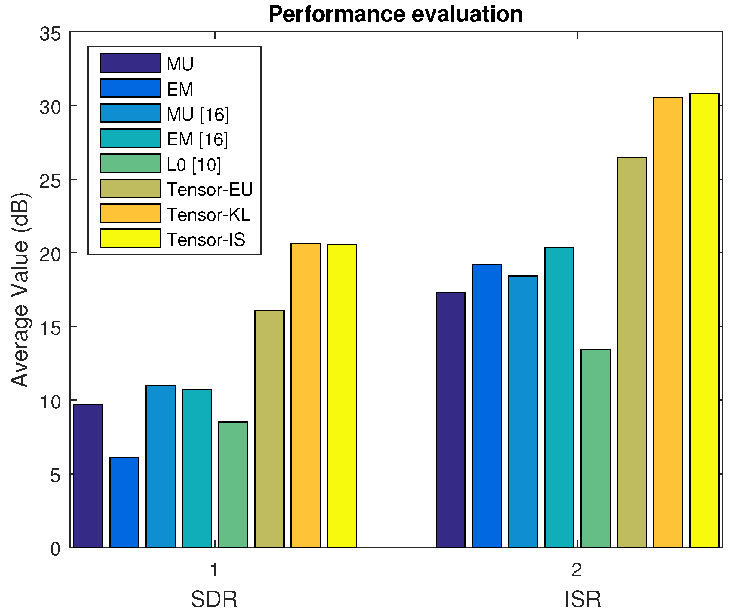
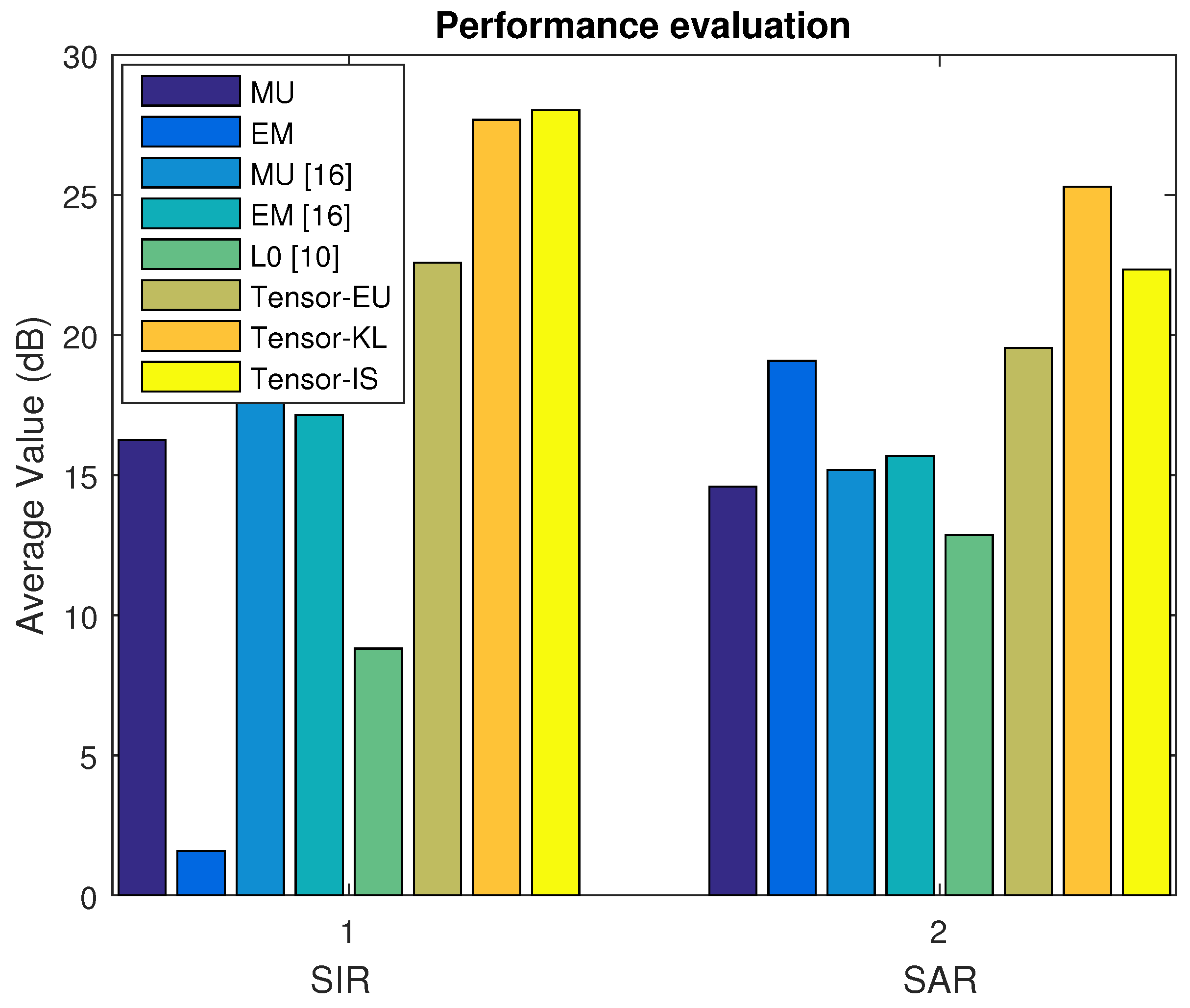
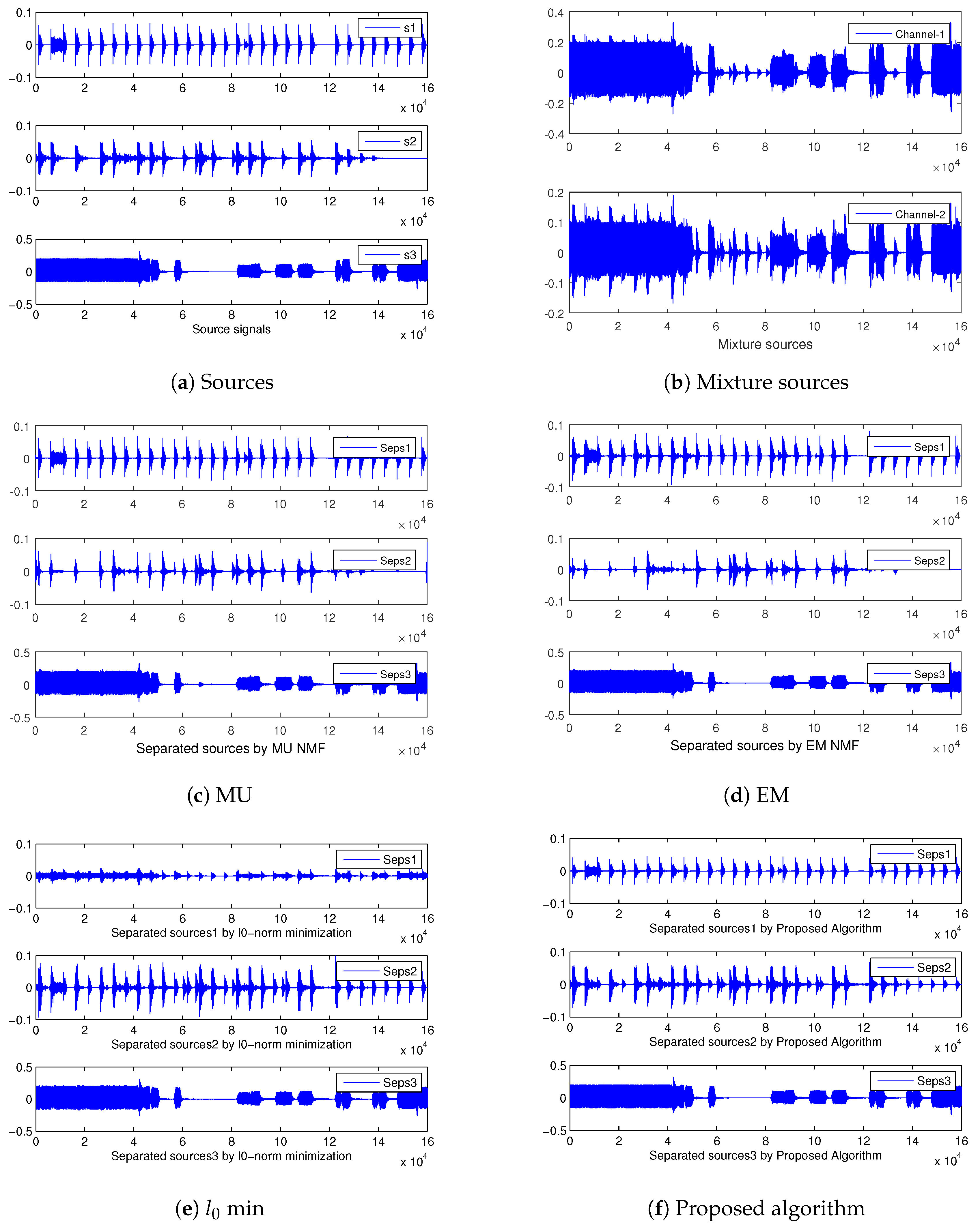
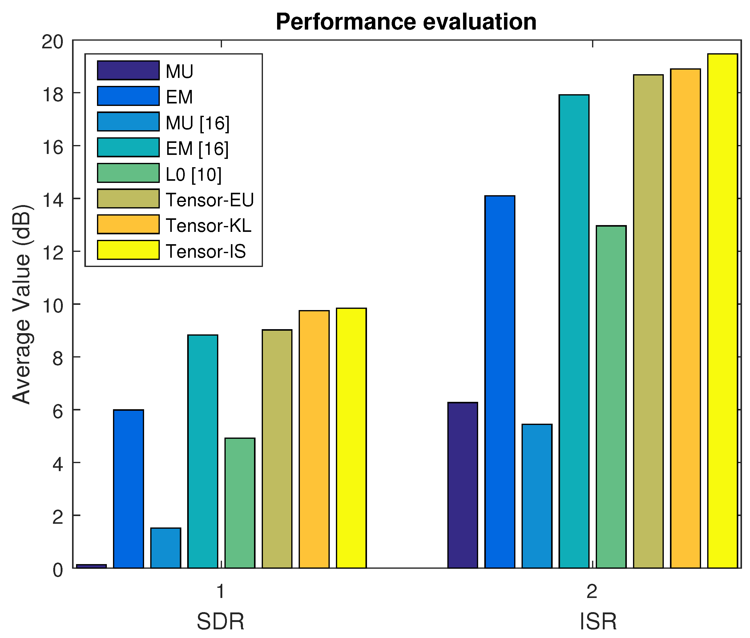
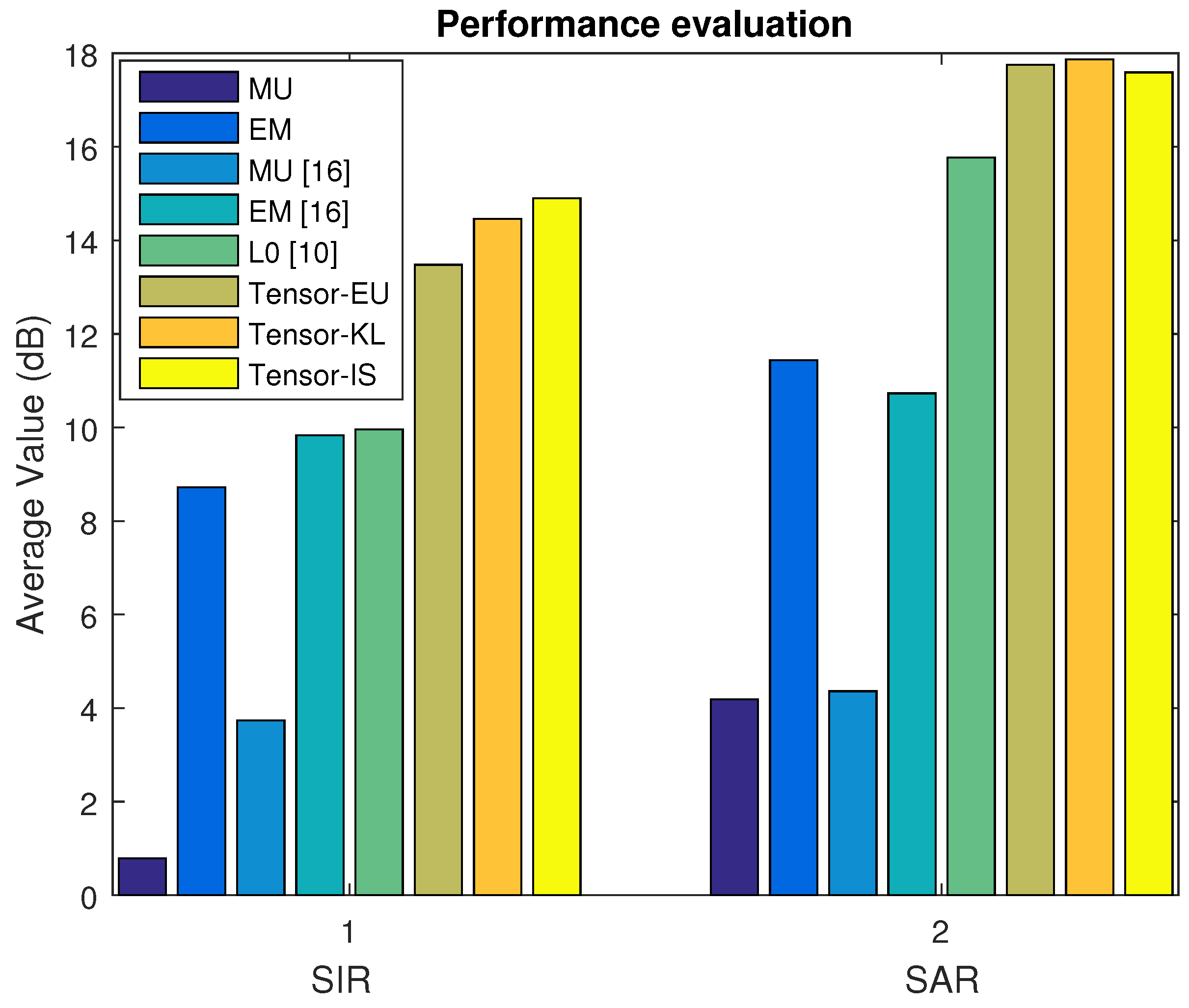
4.4.1. Music Signal Mixtures in the Linear Instantaneous Case

In Dataset A, we first select the music signal mixtures in the linear case. The average SDR, ISR, SIR, and SAR are depicted in Figure 2 and Figure 3 based on the MU, EM with the random initialization, MU [16], EM [16], $l_0$ min [10], and our proposed algorithm (Tensor-EU, Tensor-KL, Tensor-IS). Finally, the waveforms of the estimated sources are shown in Figure 4.

4.4.2. Speech Signal Mixtures in the Linear Instantaneous Case

In Dataset B, we select the speech signal mixtures in the linear instantaneous case. The average SDR, ISR, SIR, and SAR are depicted in Figure 5 and Figure 6 based on the MU, EM with the random initialization, MU [16], EM [16], $l_0$ min [10], and our proposed algorithm (Tensor-EU, Tensor-KL, Tensor-IS), respectively.

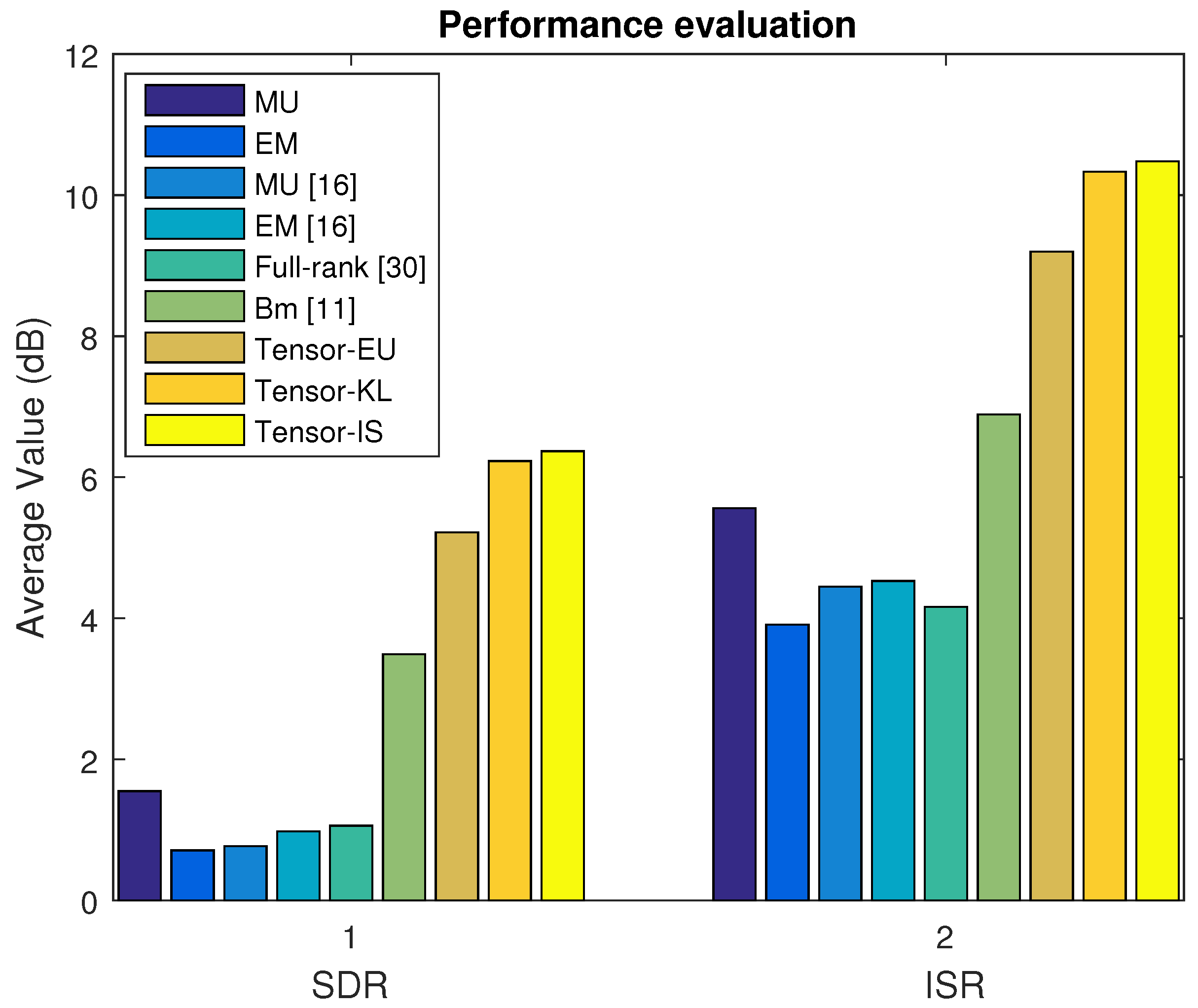
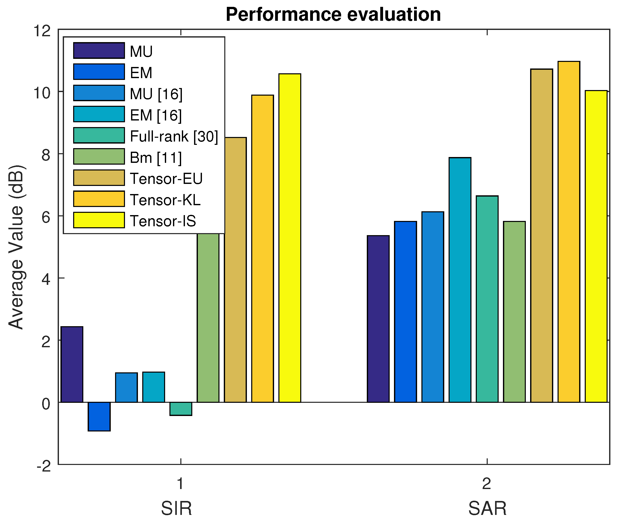
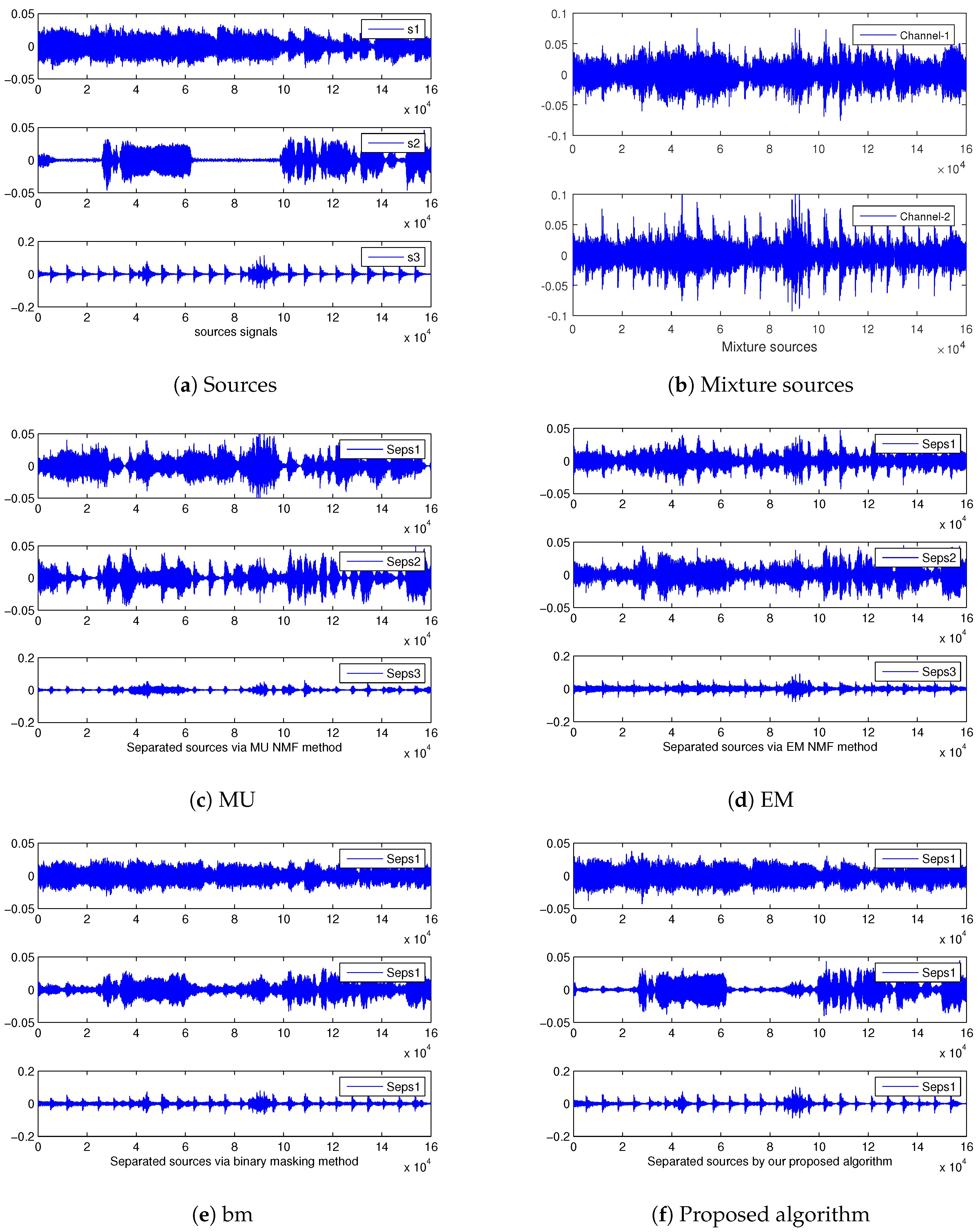
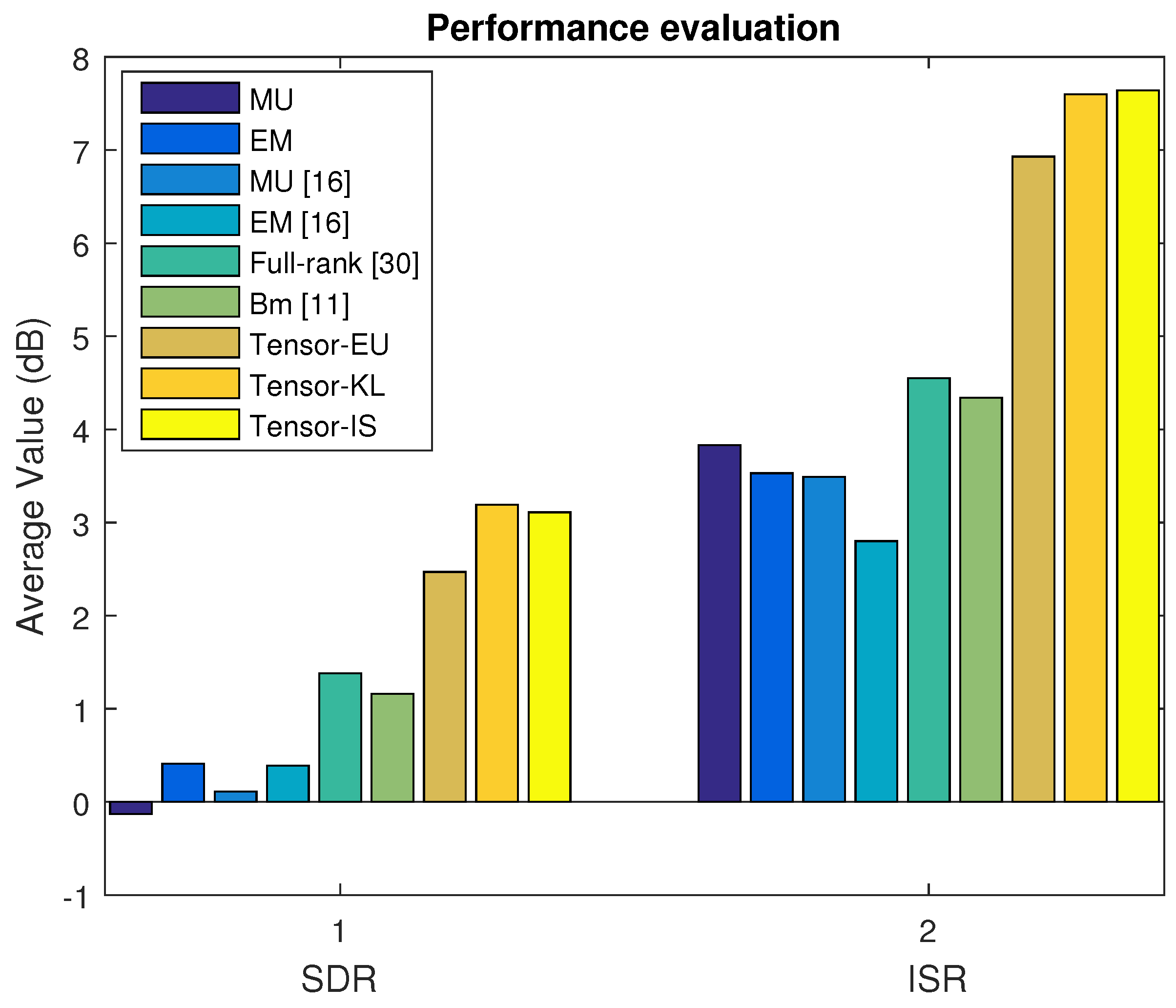
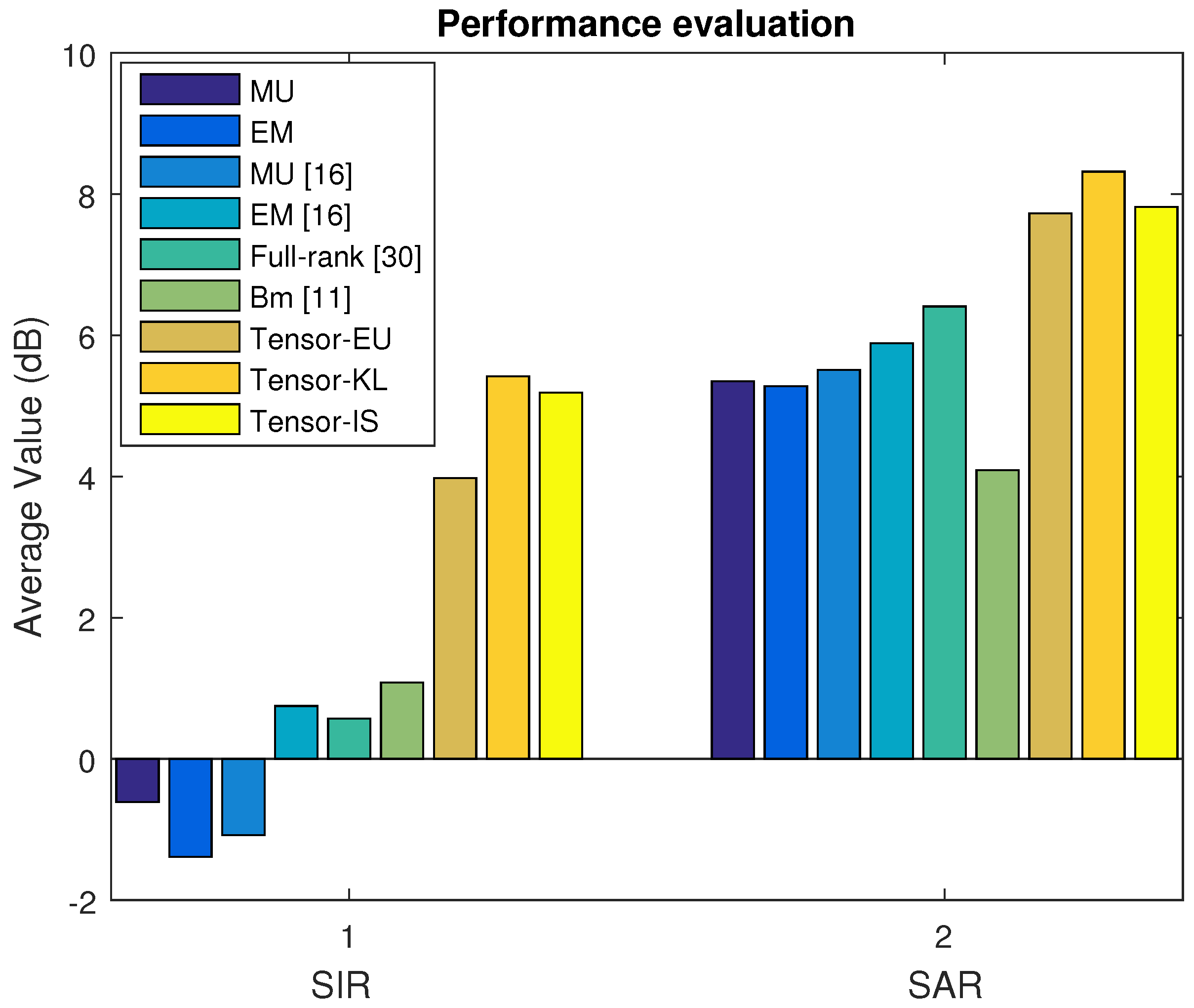
4.4.3. Music Signal Mixtures in the Convolutive Case

In Dataset C, we select the real live recording convolutive dataset which consists of vocal and musical instrument with drum. The average SDR, ISR, SIR, and SAR are depicted in Figure 7 and Figure 8 based on the MU, EM with the random initialization, MU [16], EM [16], Full-rank [30], Bm [11] and our proposed algorithm (Tensor-EU, Tensor-KL, Tensor-IS), respectively. Finally, the waveforms of the estimated sources are shown in Figure 9.

4.4.4. Speech Signal Mixtures in the Convolutive Case

In Dataset D, we select the synthetic convolutive mixtures including three speech sources and two mixing channels. The average SDR, ISR, SIR, and SAR are depicted in Figure 10 and Figure 11 based on the MU, EM with the random initialization, MU [16], EM [16], Full-rank [30], Bm [11] and our proposed algorithm (Tensor-EU, Tensor-KL, Tensor-IS), respectively.

Discussion 1. According to the above experimental results of Dataset A, Dataset B, Dataset C, and Dataset D, it can be seen that our proposed algorithm can separate music signal mixtures and speech signal mixtures in the underdetermined linear and convolutive case. What is more, according to the average value of source separation results, it is also shown that our proposed algorithm outperforms the baseline algorithms.

4.5. The Runtime of All Algorithms

The corresponding runtimes of the algorithms are shown in

Table 2. The runtime of all algorithms (sec.).

Linear BSS Case		Convolutive BSS Case
Algorithm	Runtime	Algorithm	Runtime
$l_0$ min [10]	21.3982	bm [11]	38.5658
MU [16]	65.5909	MU [16]	70.3608
EM [16]	90.5785	EM [16]	182.2820
−	−	Full-rank [30]	346.5758
Proposed	114.6651	Proposed	208.8797

. It can be seen that the proposed algorithm takes more time than the MU and EM methods. It is mainly because the time consuming on estimation of mixing matrix based on tensor decomposition. However, compared with the full-rank algorithm, our proposed algorithm takes less time. Additionally, as for the source separation results, the proposed algorithms exhibit better separation performance than the compared algorithms. In our future work, it is still necessary to develop a better algorithm to reduce time cost.

5. Conclusions and Future Work

In this paper, we proposed an optimization underdetermined multichannel BSS algorithm based on tensor decomposition and NMF. Because the EM method is very sensitive to the parameter initialization, we first estimated the mixing matrix employing tensor decomposition; meanwhile, the source spectrogram factors were estimated using NMF source model, and produced an optimization parameter initialization scheme. Then the model parameters were updated using the EM algorithm. The spatial images of all sources were obtained in the minimum mean square error sense by multichannel Wiener filtering. The time-domain sources can be obtained through inverse STFT. Finally, a series of experimental results showcase that our proposed optimization algorithm improves the separation performance compared with the baseline algorithms.

In addition, there are some aspects that deserve further study. Firstly, the estimation of number of components of NMF model is an open topic. There have been some articles to solve this problem, such as the automatic order selection [33], Information Theoretic Criteria [34], and N-way Probabilistic Clustering [35]. Secondly, the window length used in the STFT has been taken advantage to match the characteristics of audio signals, and different window lengths have different effects on the separation results. Furthermore, taking into account source or microphone motions [36,37], i.e., convolutive mixture corresponding to source-to-microphone channel that can change over time, is a challenging problem. Therefore, these problems would be the focus of our future work.