Fault Diagnosis of Mine Shaft Guide Rails Using Vibration Signal Analysis Based on Dynamic Time Warping

Abstract

Guide rails are amongst the most important components of mine hoist systems, and faults in them must be detected as early as possible to avoid fatal breakdowns in mine production. Presently, guide rail inspection is performed visually in most situations. In this paper, we examine a more efficient approach based on multi-time scale and dynamic time warping (DTW) to diagnose guide rail faults including embossment, bumps, and clearance. Firstly, vibration signals collected from operational conveyance under different fault categories are analyzed and the corresponding characteristic waveforms (CWs) are extracted. Embossment faults are identified with priority according to visible disparities in CW patterns on a large time scale. Then, templates for bump and clearance faults are established through processing the CWs on a small time scale. Subsequently, the distances of DTW (DDTWs) between test samples and the selected templates are calculated. Finally, the remaining fault conditions are classified according to the DDTW results since the same fault category has the smallest distance. Experiments are conducted on a guide rail fault simulator to demonstrate the reliability of the proposed method. The resultant diagnosis accuracies are 100%, 90.40%, and 84.53%, respectively, for embossment, bump, and clearance faults, which indicates that the proposed approach is feasible and effective for diagnosing guide rail faults under variable operating conditions and different fault severities.

1. Introduction

Guide rails are one of the most essential infrastructure components in colliery, and guide the conveyances transporting staff, materials, and ore in the wellhole [1]. A typical structure of a guiding system which consists of a conveyance and two guide rails is shown in Figure 1. Four sets of rollers are installed on the conveyance which is restrained by two guide rails. Each set of rollers comprises three singular and orthogonal rollers. In practical applications, the guide rail extending from the bottom to the top of the mine shaft is assembled from many equal-length tracks which are attached and fixed to a grid of buntons. Due to shaft deformation, improper mounting, and acid corrosion of steelwork, etc., various faults may occur in the guide rail, exciting abnormal vibrations in the conveyance and leading to dangerous situations, even catastrophic failures. Moreover, the frequent services also accelerate the guide rail deterioration process. Therefore, it is necessary to monitor the health status of and diagnose faults in the guide rail to ensure safety in coal mines [2,3,4].

Most currently employed methods for guide rail maintenance are based on visual inspections which are conducted regularly according to a prescribed schedule and which require considerable hoister downtime. The distance between two guide rails and their individual perpendicularities are widely used measurements in these methods [5]. However, on the one hand, these types of measurements are most efficient at later stages of the degradation process, and on the other hand, perfect performance in the quiescent state of the guide rail has little reference value to the operational state, which counts more for safety production management. With rich condition-related information, the vibrations of the running conveyance excited by guide rail failures provide an alternative way to deal with this problem. To date, few scholars have focused on fault detection and diagnosis from vibration signals for mine shaft guide rails. Li [6] utilized singularity analysis to detect guide rail defects, and Jiang et al. [7] applied Laplace wavelets to identify impulse responses from conveyance signals. Ma et al. [8] firstly extracted five fault features from vibration signals and then compared six classification methods to diagnose guide rail failures. This pattern recognition method requires a significant amount of learning samples, which is a limitation in practical situations. Besides this, when the operating condition varies, the effect of this method will be influenced. With similar structures, railway tracks face the same problems, and the literature in this field is relatively broader. Lederman et al. [9] proposed a sparse approach to inspecting tracks. Wei et al. [10] investigated railway alignment information based on frequency response analysis. Due to the effectiveness in analyzing nonstationary and transient vibration signals, time–frequency analysis approaches have received increasing interest. Liang et al. [11] applied four techniques including smoothed pseudo Wigner–Ville transform (SPWVT), short-time Fourier transform (STFT), Choi–Williams transform (CWT), and wavelet transform (WT) to obtain time–frequency representations of impact signals excited by rail surface defects. Caprioli et al. [12] employed continuous wavelet transformation of bogie signals for rail inspection. Molodova et al. [13] proposed an automatic detection algorithm for squats in rail infrastructure based on wavelet spectrum analysis. With these methods, railway defects can well be detected and located. Nevertheless, they are unable to classify different rail faults efficiently. As a solution, Salvador et al. [14] firstly calculated the excitation frequencies of diverse rail faults with defect wavelength and travel speed, then identified fault categories based on STFT. However, this method requires the wavelength of certain fault as a priori knowledge. When the fault severity varies with the performance deterioration, this method becomes ineffective.

In recent years, dynamic time warping (DTW) as a distance measurement technique has received considerable attention in machinery fault diagnosis. Originally proposed to improve isolated word recognition [15], it depicts the similarity between two time series which may vary with time. Zhen et al. [16] utilized DTW to analyze electrical current signals for motor condition monitoring. Sobie et al. [17] compared DTW with six commonly used machine learning methodologies in the classification accuracy of bearing failures and investigated its application in industrial fields. Huang et al. [18] developed an intelligent diagnosis method for railway turnout through DTW and achieved promising results. Han et al. [19] applied normalization to erase the influence of vibration amplitude discrepancy and classified bearing faults according to the distances of DTW (DDTWs) between targeted samples and templates. Compared with conventional data-driven fault diagnostic techniques, DTW does not require feature selection and algorithm training; the critical step is to extract the representative template from limited historical signals.

From the literature mentioned above, it can be seen that guide rail monitoring has mainly been focused on fault detection using signal processing techniques; few works have shown fault classification from different categories. Considering the variable operating conditions, the mentioned existing pattern recognition method and characteristic frequency identification method are not suitable for guide rail fault diagnosis. For solving this issue, this paper presents a novel diagnostic approach based on a multi-time scale technique and DTW. The engineering novelty of this article is to eliminate the influence of variations in lifting parameters and fault conditions in order to realize accurate guide rail fault diagnosis. A flowchart of the proposed method is shown in Figure 2. Firstly, the primordial vibration signals under varying operating conditions are obtained from a guide rail fault simulator. Then, the characteristic waveforms (CWs) at defect points are extracted from the raw signals and analyzed on a large time scale. Typical fault types are discerned due to obvious manifestations of impulse numbers. Subsequently, standard templates for remaining fault categories are established through processing the CWs on a small time scale. Finally, the similarities between the test data and the standard templates are calculated through DTW and the remaining fault types are classified with the resultant DDTW.

The remainder of this paper is structured as follows. Section 2 presents the fundamentals of DTW. In Section 3, the experimental setup is described in detail and vibration signals are acquired. Results and discussion are given in Section 4, and some conclusions of this study are drawn in Section 5.

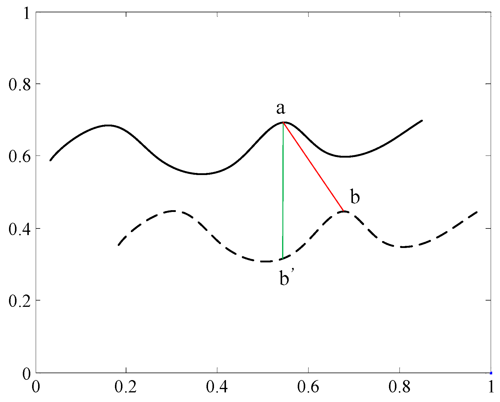
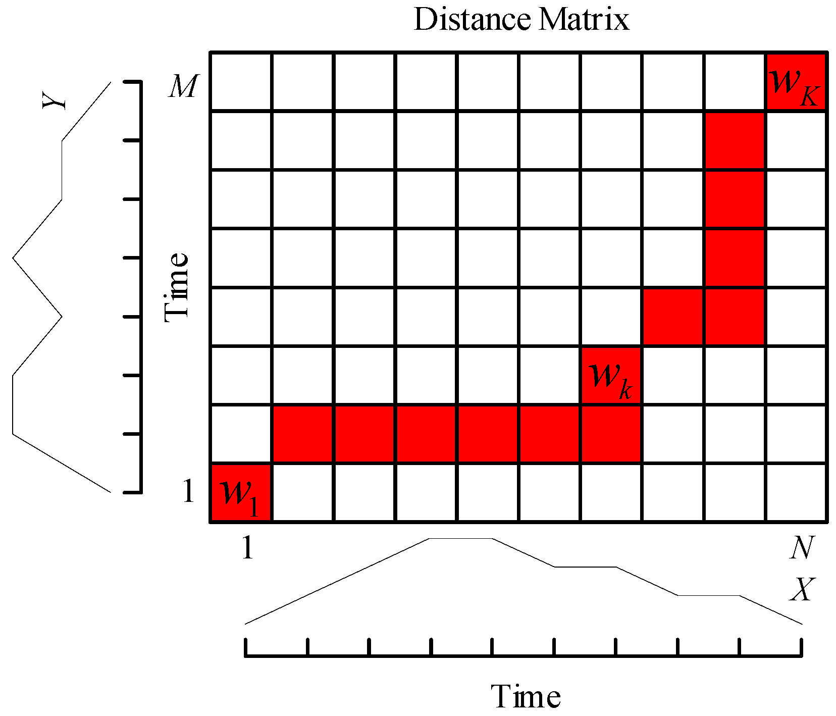
2. Dynamic Time Warping

DTW aims to find the optimal path between two time series by allowing them to be warped nonlinearly in the time dimension [20]. Different from the Euclidean distance (ED), DTW is suitable for handling series with diverse lengths. An example to show the distinction between ED and DDTW is presented in Figure 3. Two lines have high similarity exclusion of position. Point a is one peak of the solid line. Point b’ is the corresponding spot in the dotted line using ED, while point b is identified which correlates to point a in DDTW. From the aspect of physical sense, DDTW is more proper to describe the similarity between two time series.

The basic principle of DTW is delivered as follows [21]. Given two time series of length N and M,

$$X=x_1,x_2,\cdots ,x_i,\cdots ,x_N$$

(1)

$$\mathrm{and}Y=y_1,y_2,\cdots ,y_j,\cdots ,y_M.$$

(2)

To align the two time series for comparison, a two-dimensional distance matrix D of dimension N × M is constructed first, whose elements $d(x_i,y_j)$ are the distances between two points x_i and y_j.

Once the distance matrix is built, the warping path W is determined by calculating the minimal cumulative distance between the time series:

$$W=(w_1,w_2,\cdots ,w_k,\cdots ,w_K)$$

(3)

where $K$ is the length of the warping path, $\max (N,M)\le K\le N+M$. The kth element of the warping path is

$$w_k=(i,j)$$

(4)

where $i=1,2,\cdots ,N$ is an index from time series $X$ and $j=1,2,\cdots ,M$ is an index from time series $Y$.

The warping path must satisfy the following three constraints [18,20]:

• Boundary condition: $w_1=(1,1)$ and $w_K=(N,M)$. The warping path must start at the beginning and finish at the end of each time series.
• Monotonicity condition: if $w_k=(n_k,m_k)$ and $w_{k+1}=(n_{k+1},m_{k+1})$, then $(n_{k+1}-n_k)\ge 0$ and $(m_{k+1}-m_k)\ge 0$.
• Continuity condition: if $w_k=(n_k,m_k)$ and $w_{k+1}=(n_{k+1},m_{k+1})$, then $(n_{k+1}-n_k)\le 1$ and $(m_{k+1}-m_k)\le 1$.

The optimal warping path can be calculated by using a dynamic programming approach following the iteration below:

$$\lambda (i,j)=d(x_i,y_j)+\min \left\{\lambda (i-1,j-1),\lambda (i-1,j),\lambda (i,j-1)\right\}$$

(5)

where $d(x_i,y_j)$ is the element in the current cell of matrix D, and $\lambda (i,j)$ is the sum of $d(x_i,y_j)$ and the minimum cumulative distances from three adjacent cells. Figure 4 shows an example to determine the optimal warping path based on the distance matrix for the alignment of two time series. The DDTW between time series $X$ and $Y$ is the sum of the matrix elements in the warping path W.

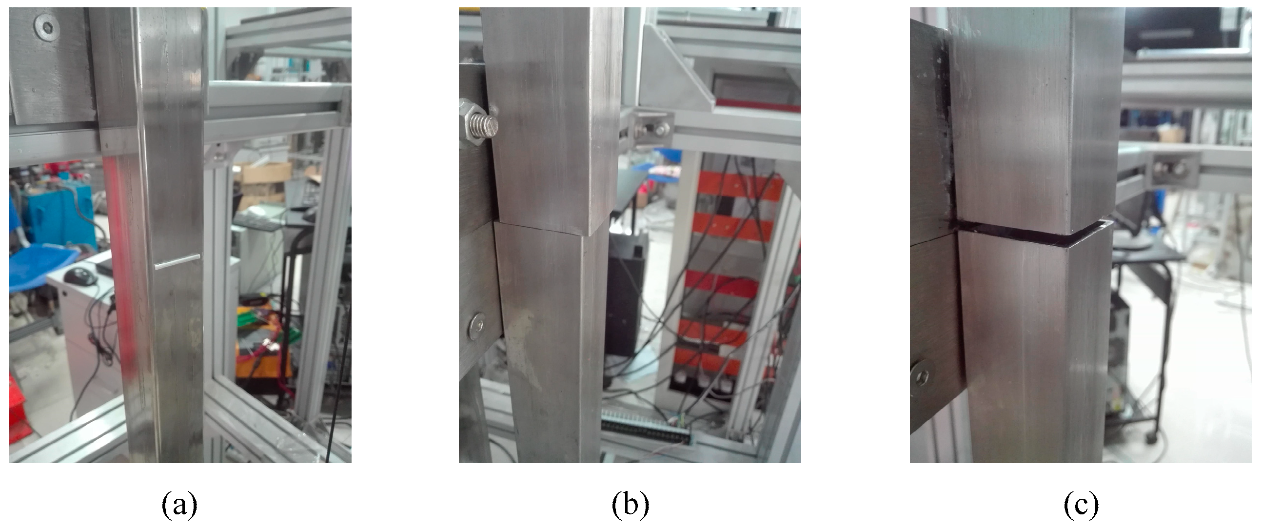
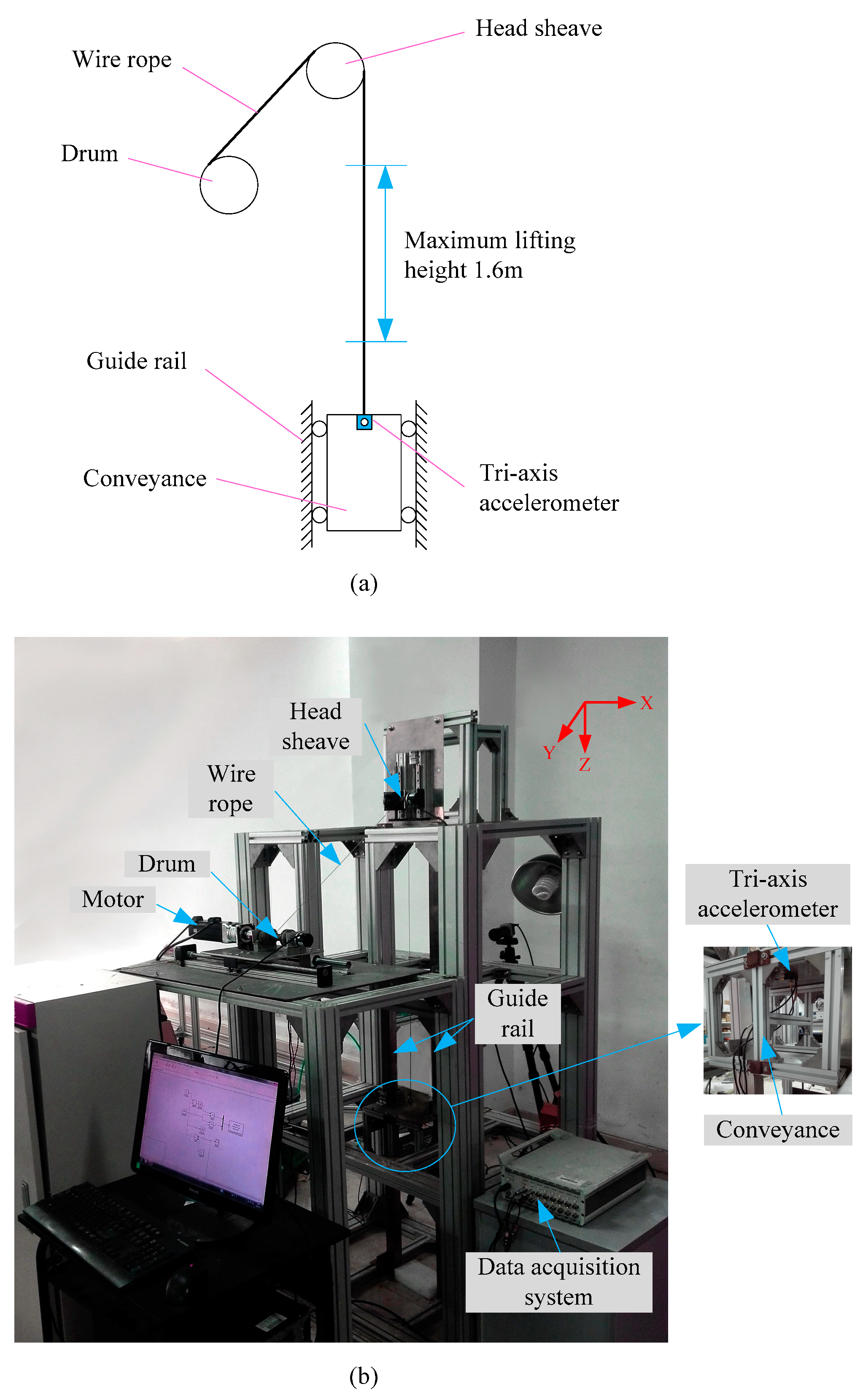
3. Experimental Setup

According to the difference in fault modality, guide rail failures can be roughly classified into two types: slow-changing failures and impact failures. Slow-changing failures, including inclination and deformation, affect the conveyance in a relatively moderate way. This is because the fault region is always large; thus, the conveyance is less influenced when operating in a small portion of the fault area. Embossment, bump, and clearance, shown in Figure 5, are three typical cases of impact failures. Almost all the fault causes which finally excite impulse signals, such as solid attachment and bolt looseness, are manifested through these three failures. Due to the fact that impact failure concentrates on a small defect point, it can excite abnormal vibrations and even result in rope breaking, conveyance jamming, or falling. Therefore, it is necessary to diagnose the impact failures, investigate the fault causes, and then form the corresponding maintenance strategies before an accident occurs. Considering the serious consequences, impact failure diagnosis is focused upon in this paper.

To demonstrate the effectiveness of the proposed method, experiments were developed on a guide rail fault simulator. The principle and the physical photos of the simulator are shown in Figure 6. With a head sheave mounted on its top, the metal framework is equipped with two guide rails which guide the conveyance to move along the vertical direction. The drum is connected to a motor for providing power to the simulator. A steel wire rope wraps around the head sheave with the conveyance hanging on one end and the other end bent over the drum. The diameter of the roller is 19 mm, and the mass of the roller is 8 g. The stiffness and damping of the roller buffer device are 0.12 KN/mm and 0.03 KN·s/mm, respectively. One tri-axis accelerometer was installed beneath the top surface of the conveyance to obtain the vibrations in three directions at the sampling rate of 20 KHz. A description of the accelerometer is exhibited in

Table 1. Specification of the accelerometer.

Type	Manufacturer	Sensitivity (mV/m·s−2)
		X	Y	Z
DH311E	Donghua Testing	1.09	1.19	1.05

. The acceleration data was sampled by a DH5922 data acquisition system with 16 channels, 24-bit resolution, and a maximum sampling rate of 256 KHz. Due to the high magnitude and the concentrated frequency of the content [22], the vibration data from the z axis was applied to demonstrate the proposed method in this paper.

Aiming at diagnosing guide rail faults under different operating conditions, the scheme of this experiment was designed as shown in Figure 7. Four factors were considered including lifting speed (5 types), lifting load (5 types), fault category (3 types), and fault severity (3 types). By adding a normal case, the total number of experimental cases is 5 × 5 × 3 × 3 + 1 = 226.

In order to verify the proposed approach and to eliminate the effects of random interference, each case was implemented five times.

4. Results and Discussions

4.1. CW Selection

CW is the trimmed signal on which different failures are evidently distinguished from each other. It contains the most useful information for fault diagnostic decision-making. The selection of CW is the premise of the proposed method. Due to the distinct fault shape, the dynamic contact force between the rollers and guide rails at the defect point is different, which leads to a discrepancy in the patterns of vibration signals. Therefore, the time-domain CW is an intuitive but critical indicator to represent various types of guide rail faults. For the sake of extracting the CWs for the aforementioned failures, the experimental data were carefully analyzed.

4.1.1. Normal Condition

To set a reference, an original vibration signal of the normal guide rail is shown in Figure 8. The lifting process experienced three stages, i.e., the startup phase, the steady phase, and the shutdown phase. In this study, the conveyance was restricted to passing by the guide rail defect in the steady phase. The reason for this restriction is that the dynamic force between roller and guide rail at the defect point in the startup phase and shutdown phase is more complex than that in steady phase; this will affect the shape of the CW and reduce the fault classification accuracy. Moreover, in practical situations, the operating time of the steady phase is relatively longer than the total time of startup and shutdown phases for a mine shaft hoist system.

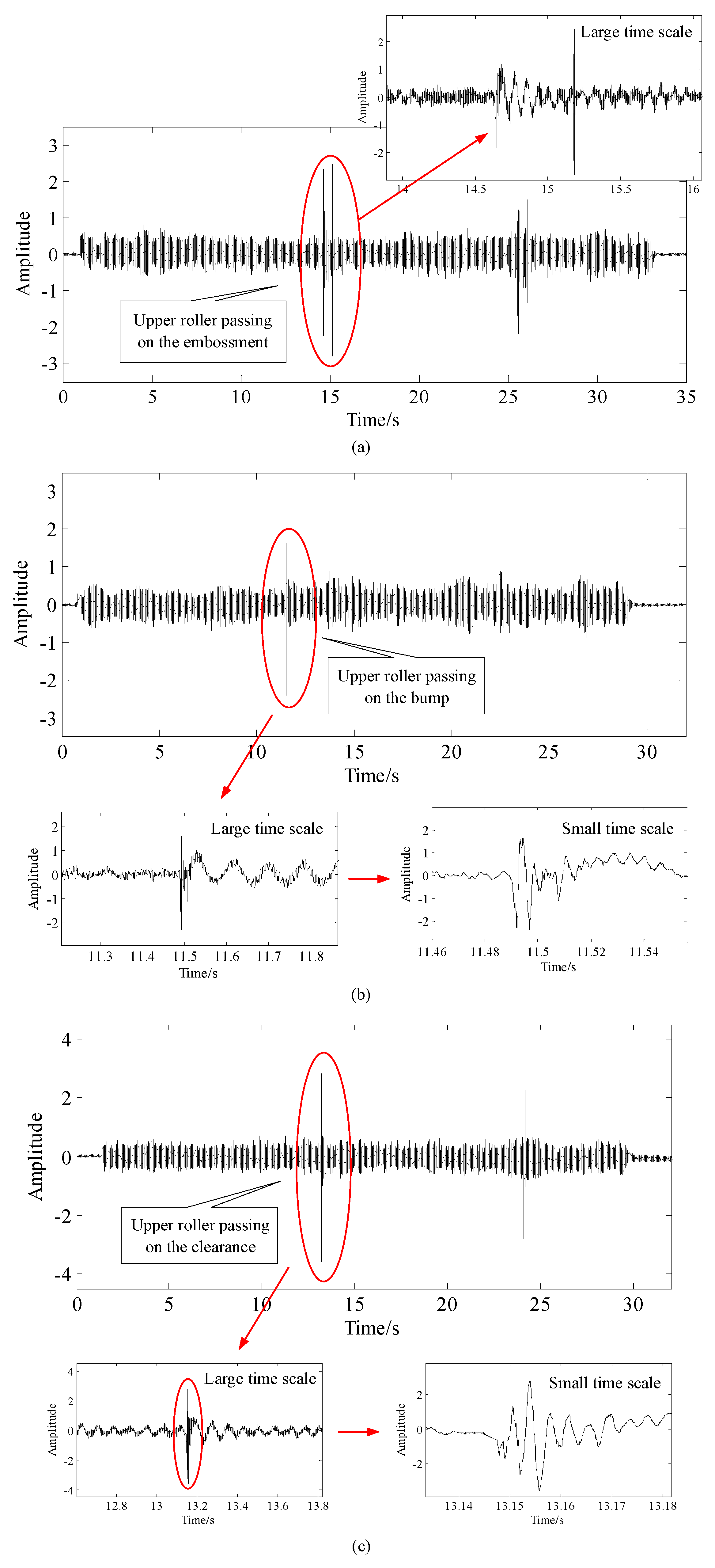
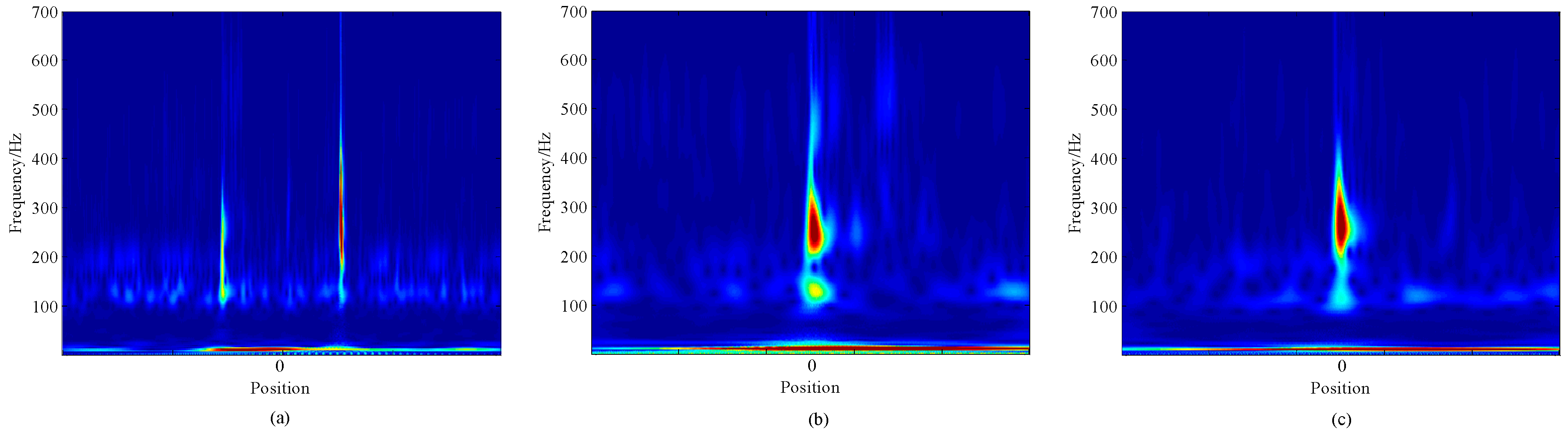
4.1.2. Fault Conditions

Figure 9 presents original signals under three different guide rail faults and their corresponding enlarged views on multiple time scales.

It is obvious from this figure that there exist two sets of impulses in each primordial signal, regardless of fault categories, which are excited by the upper and lower guide rollers of the conveyance, respectively. The reason for the amplitude difference between the two observed sets of impulses is that the stiffness and damping of the roller buffer device are different. In this paper, the first set of impulses was selected for guide rail diagnosis. From the trimmed signals on a large time scale, we can see that the embossment fault is distinguished from bump and clearance because two bursts emerged; due to this, the embossment fault can be classified with priority. In fact, the first burst is considered as the defect commencement when the guide roller strikes the embossment, while the second burst represents the defect exit at the moment at which the guide roller moves away from the trailing edge of the embossment and hits the guide rail. Although one burst appears in both enlarged signals of the remaining two fault types on a large time scale, the localized waveforms on a small time scale are predominantly distinct and can be regarded as the CWs of bump and clearance faults. The generating mechanisms of the detailed waveforms lie in collision for the bump fault [23] and in de-stressing and re-stressing for the clearance fault [24,25,26,27].

Signals relating to embossment, bump, and clearance faults at defect points were processed using wavelet transform. The time–frequency representations are shown in Figure 10. The bright color indicates a high signal energy level that is caused by an impact. Embossment fault can be easily classified according to the appearance of two high-energy areas, which corresponds to the evidence given by the time-domain waveform. The frequency components and maximum frequency ranges of the bump and clearance faults are similar, and the detailed differences on a small time scale at defect points cannot be depicted in Figure 10b,c. Besides this, the bright areas vary with lifting speed [28], lifting load [29], and fault severity [13], which confuses the time–frequency analysis and makes it difficult to classify bump and clearance faults from time–frequency representations. Salvador et al. [14] successfully identified diverse rail faults through recognizing fault characteristic frequencies in an STFT spectrogram; the key point is that the frequencies excited by different defects are known in advance and the frequency ranges are isolated, whereas the frequencies excited by bump and clearance faults in this paper under different operating conditions are unknown and may be overlapped.

In conclusion, four health conditions of guide rails were investigated above, including normal, embossment, bump, and clearance; these conditions show great differences in time-domain waveforms at defect points. The embossment faults can be firstly distinguished according to the number of bursts on a large time scale. On the other hand, the waveforms on a large time scale and the time–frequency representations of bump and clearance faults are similar; thus, these two categories of failures remain to be differentiated through further processing on a small time scale.

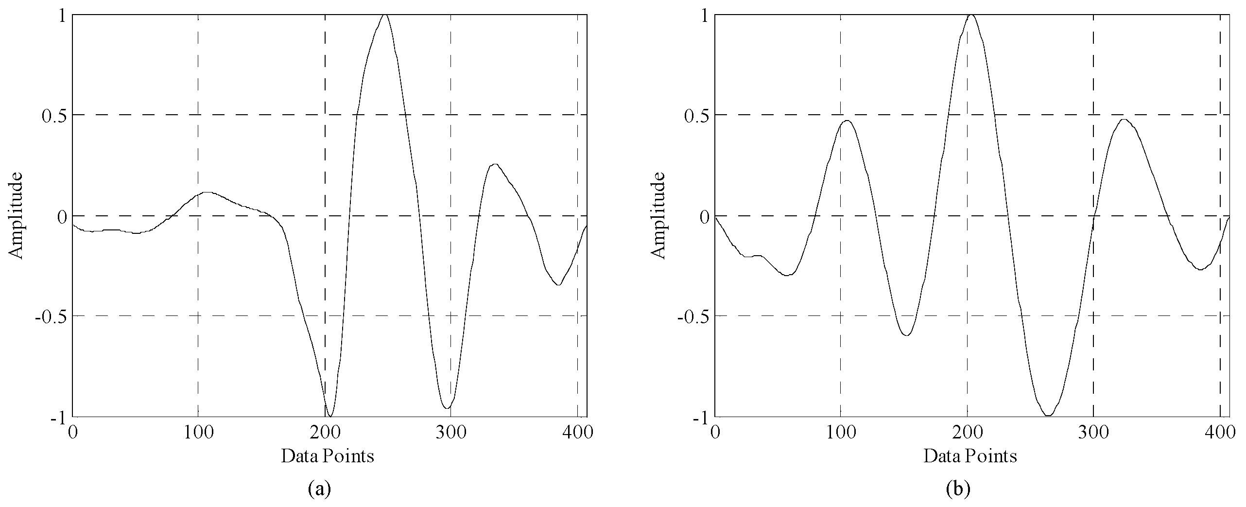
4.2. Template Establishment

The establishment of templates for bump and clearance faults is the most essential procedure in the proposed method and affects the accuracy of diagnosis directly. The extracted CW is a raw and truncated signal that contains extensive interference. It is necessary to process the CW to obtain a standard template. For the purpose of removing the noise in the CW and improving fault diagnosis accuracy, the following steps were carried out.

1. CW Selection:

The primordial signal of the entire lifting process contains a large segment of vibrations irrelevant to guide rail fault. For the sake of removing the useless waveforms, the CW as a strip of a duration which covers the first burst is extracted.

2. De-trend:

Due to the measurement deviation of the transducer, the disturbance of the working environment, and the oscillation of the conveyance, a nonlinear trend term which varies with operating conditions and introduces large distractions is inevitable in the extracted CW. In this case, a polynomial method based on least squares is utilized to eliminate this influence.

3. Averaging:

In order to alleviate the random interference and make the de-trended CW more representative, an averaging technique is performed. Herein, the respective means of the five repeated samples under the same operating condition are computed for bump and clearance faults. The key point of averaging is to identify the exact moment at which each stimulus occurs [13].

4. Smoothing:

The averaged signal still contains a portion of an unwanted high-frequency component which disturbs the calculation of the DDTW. Thus, a moving average algorithm is an easy but efficient way to remove the high-frequency noise and smooth the signal [30]. The criterion of this step is to strike a good balance between suppression of noise and preservation of the waveform, which is crucial for decision-making.

5. Interception:

The CW extends on both sides with several small fluctuations which will confuse the result of the DDTW and deteriorate the efficacy of diagnosis. The critical component for classification is the signal segment carrying a whole burst which represents the fault property. Therefore, the smoothed CW should be intercepted according to certain principles. Taking both CWs of bump and clearance faults into consideration, the procedures below are conducted.

• Set the reference line L = 0.
• Pick the point of maximum amplitude O from the pattern of the smoothed CW.
• Define Spot A when the smoothed CW crosses L the fourth time from Point O on the left as the start point of the template.
• Define Spot B when the smoothed CW crosses L the fourth time from Point O on the right as the end point of the template.

6. Normalization:

It is apparent that the CW magnitudes change with different operating conditions, which will severely affect the range of the DDTW and produce a high misclassification rate. In order to eliminate the influence of amplitude variations and make the proposed diagnostic method universal, it is necessary to normalize the intercepted CW through the following transformation function:

$$\tilde{x}=\frac{x-x_{\min }}{x_{\max }-x_{\min }}$$

(6)

where $\tilde{x}$ is the normalized value, $x$ is the original value, $x_{\max }$ is the maximum value, and $x_{\min }$ is the minimum value.

For brevity, the signal processing scheme is pictorially presented in Figure 11 (taking a bump fault as an example).

After performing the procedures of the signal processing approach detailed above, the templates of bump and clearance faults were obtained. To make a fair comparison, the clearance template was subsequently processed through a linear interpolation algorithm to ensure the same number of data points as the bump template. Lastly, the standard templates of both faults were established for DDTW calculation as shown in Figure 12. It can be seen from this figure that the patterns of these two templates vary from each other distinctly; this is considered as evidence of guide rail fault classification. For a bump, the impact event caused by collision changes the direction of the guide roller almost instantaneously, while for clearance, the de-stressing event affects the guide roller incrementally.

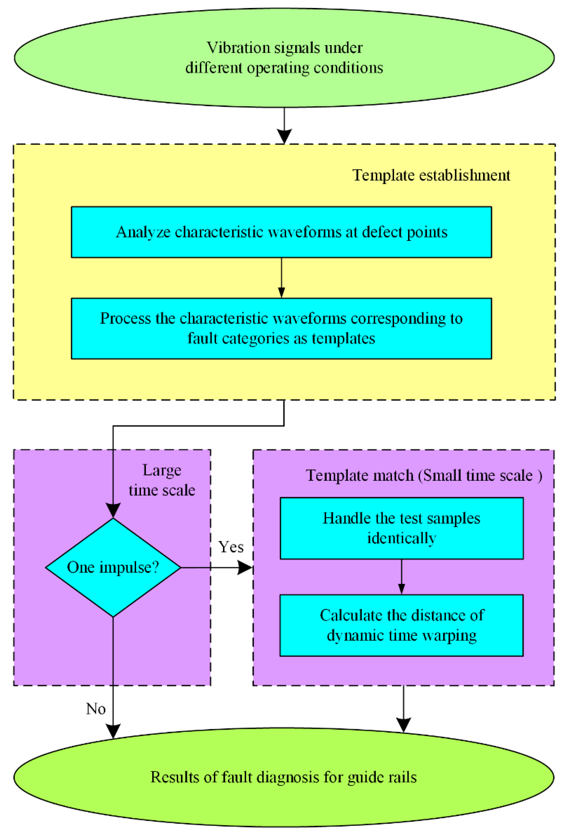
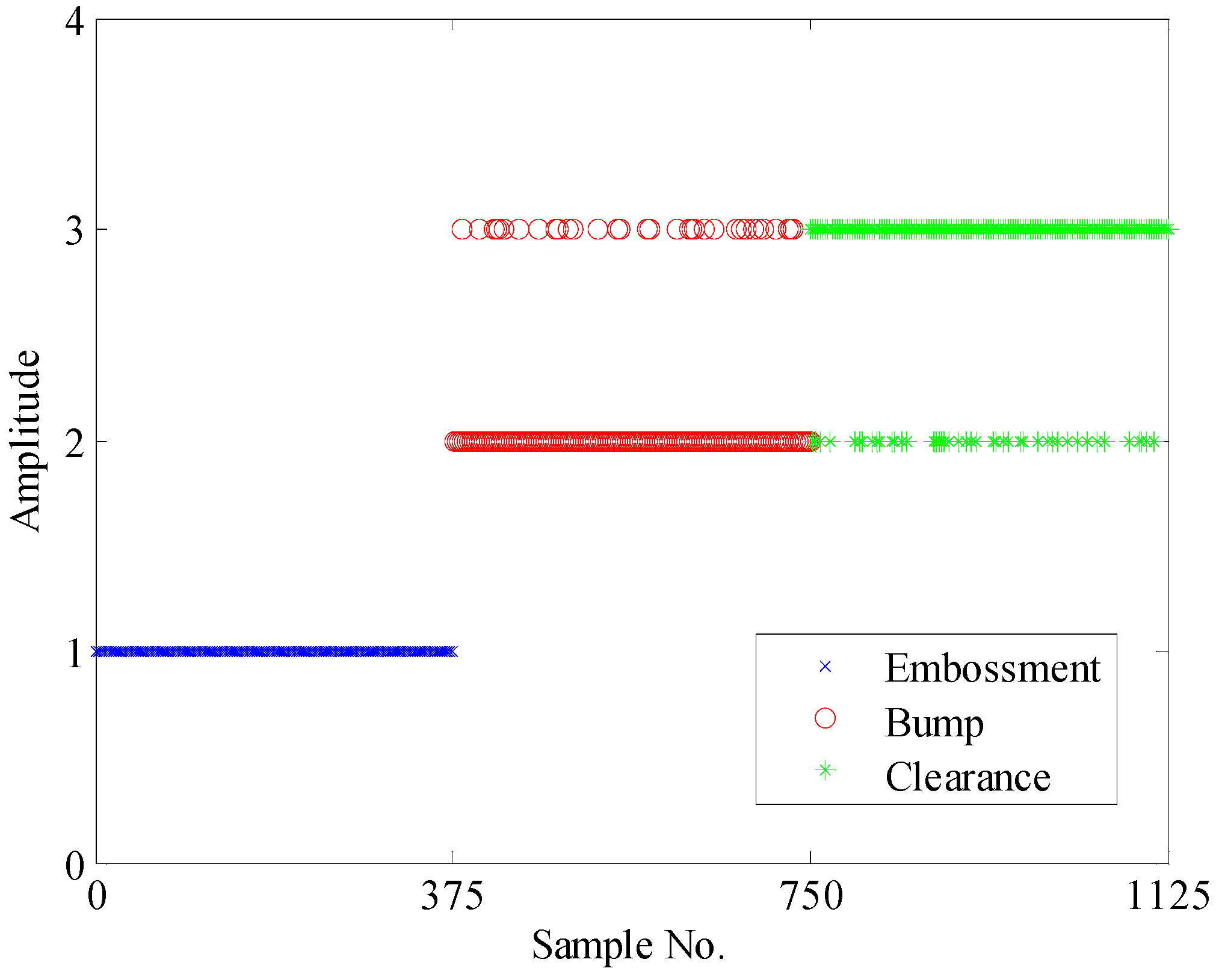
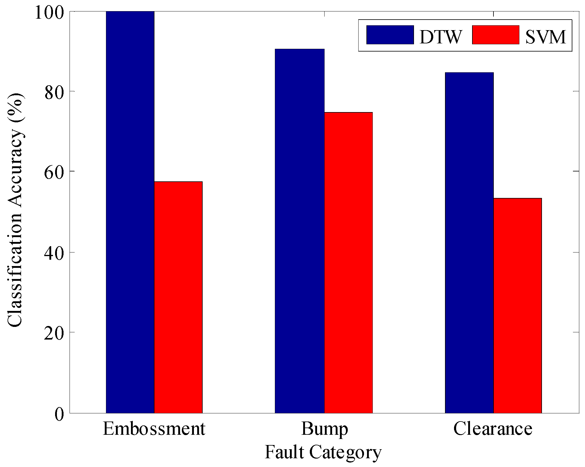
4.3. Fault Diagnosis Based on the Proposed Method

In this study, 225 kinds of faulty operating conditions for conveyance were considered as shown in Figure 7, and each condition was experimentally produced five times. Therefore, the total number of tests for fault conditions was 225 × 5 = 1125.

All these vibrations divided into the three fault categories were utilized to verify the validity of the proposed method. It should be pointed out that due to different lifting speeds, lifting loads, fault categories, and fault severities, the amplitude and point number of the CW for each operating condition are different.

The test samples under embossment fault were firstly picked out on a large time scale. The remaining samples after identical preprocessing were compared with the templates shown in Figure 12 through the DTW algorithm on a small time scale. In order to make the diagnostic results more intuitive and more easily observed, a simple logic rule was defined as follows:

$$P=\{\begin{array}{l}1 \mathrm{when} NI=2\\ 2 \mathrm{when} DB<DC, NI=1\\ 3 \mathrm{when} DC<DB, NI=1\end{array}$$

(7)

where NI denotes the number of impulses, DB is the DDTW between the test sample and the standard template of a bump, and DC is the DDTW between the test sample and the standard template of a clearance. P represents the fault identification indicator. P = 1 means that the embossment fault occurs, P = 2 means that the bump fault occurs, and P = 3 means that the clearance fault occurs.

With the logic rule described in Equation (7), the fault identification indicators of the test samples were calculated, and the results are shown in Figure 13. In this figure, the plots with sample Nos. 1–375, 376–750, and 751–1125 are the values of the fault identification indicators of embossment, bump, and clearance, respectively. For the plots of the test samples with Nos. 1–375, all the values of the indicator P are 1, which indicates that the test samples with Nos. 1–375 were all classified under the embossment fault. For the plots of the test samples with Nos. 376–750, 36 bump samples were misclassified as clearance faults. For the plots of the test samples with Nos. 751–1125, 58 clearance samples were misclassified as bump faults. Two bursts excited by upper and lower rollers are obvious evidence of embossment fault, which differs distinctly from the other faults. Thus, this fault category can be recognized with 100% accuracy. The discrimination between bump and clearance faults is completely dependent on the distances of DTW between the waveforms at the defect points and the standard templates. Due to the fact that the waveforms may be influenced by lifting speed, lifting load, fault severity, and disturbance from the experimental system, misclassifications appear in both bump and clearance fault categories. The diagnosis accuracies are 100%, 90.40%, and 84.53%, respectively, for embossment, bump, and clearance faults, which is an acceptable result for engineering applications.

For the sake of making the classification process easier to understand, ten test samples including five bump faults and five clearance faults were randomly selected as an example and the results are summarized in

Table 2. Results of the DTW algorithm between test samples and standard templates.

Test No.	Label	DB	DC	Classification	Result
1	Clearance	28.26	15.21	Clearance	Correct
2	Bump	15.42	38.79	Bump	Correct
3	Bump	37.62	66.30	Bump	Correct
4	Clearance	31.99	8.02	Clearance	Correct
5	Bump	26.80	44.27	Bump	Correct
6	Clearance	21.93	13.18	Clearance	Correct
7	Clearance	15.06	26.96	Bump	Incorrect
8	Bump	10.95	47.30	Bump	Correct
9	Clearance	35.26	16.20	Clearance	Correct
10	Bump	24.61	50.22	Bump	Correct

DB and DC are the DDTWs between the test sample and the standard templates of a bump and a clearance, respectively.

. A smaller distance between the test sample and the standard template indicates larger similarity. By comparing the distances from the bump template and the clearance template, the fault categories of the ten samples are easily classified.

In order to show the significance of the proposed signal processing technique when establishing the templates, a comparative analysis was conducted. Since the embossment fault has already been recognized on a large time scale, the comparison only involves bump and clearance faults which should be classified on a small time scale. Similar to in [18], the entire signals of the bump and clearance faults were regarded as templates. With a high sampling rate, the entire signals contain a large amount of data. Due to the construction of the distance matrix and the iterative calculations of dynamic programming in performing the DTW, the disadvantage of superfluous points in the time series is magnified, leading to a heavy computational burden [31]. To solve this problem, down-sampling by a factor of 30 was employed. Thereafter, the down-sampled signal was interpolated and processed using the following transformation function to ensure that all test samples and templates were on a similar scale:

$$\widetilde{x_i}=\frac{x_i}{{\displaystyle \sum _{i=1}^N\left|x_i\right|}}$$

(8)

where $\widetilde{x_i}$ is the transformed value, $x_i$ is the original value, and $N$ is the number of points. Note that the normalization depicted in Equation (6) is improper for scaling the entire signal because the randomness of the maximum value and minimum value will result in distortion of the transformed signal. The classification accuracies of both bump and clearance faults without the proposed signal processing technique are nearly 50%, indicating that the comparative method fails to classify these two failures. This is because the entire signal introduces heavy noise and contains a large segment of vibrations irrelevant to guide rail fault, which weakens the effect of the crucial waveform at the defect point on fault classification and leads to a high misclassification rate. Besides this, by using a server equipped with five Intel^® Xeon^R E5-2650 CPUs @ 2.30 GHz, 252.3 Gb RAM, and CentOS 6.5, the computing time of the algorithm with the proposed signal processing technique is 38.42 s, while the comparative algorithm takes 81,176.75 s—considerably longer. The relatively short computing time makes the proposed method adequate for diagnosing guide rail faults online. Thus, the proposed signal processing technique is indispensable in the DTW-based diagnosis method for improving the classification accuracy and saving a lot of computing time.

Meanwhile, the superiority of the proposed method is further demonstrated in Figure 14 by comparison with support vector machine (SVM) [32]. Firstly, four features were extracted from each original signal: the maximum value, the mean value, the maximum value of wavelet transform modulus maximum, and the area between the curve of wavelet transform modulus maximum and its envelope [8,32]. Then, an SVM was applied as a classifier to realize fault classification. The samples from each fault category under all conditions were randomly divided into two parts—a training set and a testing set—the proportions of which were set to 80% and 20%, respectively. In fact, this is a conventional feature-based method which is widely used in mechanical fault diagnosis. From Figure 14, we can see the DTW algorithm outperforms the SVM in terms of classification accuracy. The reason for this may be that the extracted features from vibration signals are dispersed over a large range due to variations in lifting speed, lifting load, and fault severity, and the feature values are influenced by the portion of vibrations without fault. Besides this, the computing time was 9564.37 s, and most computational resources were spent acquiring the wavelet coefficients. From the point of view of classification accuracy and time consumption, the proposed DTW method is more applicable than the comparative SVM method to the diagnosis of guide rail faults under variable operating conditions with satisfying accuracy.

Based on the above analysis, the effectiveness of the proposed signal processing technique is demonstrated and the outstanding capability of the DTW-based method is validated under different operating conditions.

5. Conclusions

Accurate guide rail fault diagnosis is regarded as a key precaution in colliery, one which can prevent unexpected failures and minimize overall maintenance costs. However, on the one hand, frequency identification methods are ineffective at diagnosing guide rail faults under diverse operating conditions, which is a typical case of characteristic-frequency-unknown problems. On the other hand, feature-based pattern recognition approaches suffer from variation in operating conditions and interference by segmental vibrations irrelevant to guide rail fault. To solve this issue, this paper presented a novel method combining a multi-time scale technique and a DTW algorithm. Firstly, the structure of the CW and the corresponding generating mechanism at the defect point for each fault category were analyzed. Then, the embossment fault was recognized with priority due to the remarkable distinction of impulse numbers in the CW on a large time scale. Subsequently, standard templates for bump and clearance faults were constructed through the proposed signal processing technique on a small time scale. Finally, the remaining test samples under bump and clearance faults were classified with the calculation of the DDTW.

To examine the performance of the proposed approach, experiments with variable operating conditions (lifting speed, lifting load, fault category, and fault severity) were conducted on a guide rail fault simulator. The results showed that the proposed method was able to efficiently identify the guide rail faults under different lifting parameters and fault conditions with diagnosis accuracies of 100%, 90.40%, and 84.53%, respectively, for embossment, bump, and clearance faults. The advantage of this method lies in the fact that the decision-making waveforms excited by guide rail faults are extracted and other partial data is discarded. In addition, DTW can align time series to erase the influence of speed variations, and normalization can scale the CWs to remove the effect of amplitude variations. Besides this, the method in [19] requires the number of points in the CWs to be the same as that in the corresponding fault template, but the proposed method is free from this strict requirement.

References

1. Khan, M.M.; Krige, G.J. Evaluation of the structural integrity of aging mine shafts. Eng. Struct. 2002, 24, 901–907. [Google Scholar] [CrossRef]
2. Krige, G.J.; Kemp, A.R. The behaviour and design of mineshaft steelwork and conveyances: A summary of a current research programme. J. S. Afr. Mech. Eng. 1982, 32, 163–169. [Google Scholar]
3. Zhu, Y.J. Research on Vertical Hoist Steelwork Guide Status Monitoring and Health Diagnosis. Master’s Thesis, China University of Mining and Technology, Xuzhou, China, 2014. [Google Scholar]
4. Krige, G.J. Some initial findings on the behaviour and design of mine-shaft steelwork and conveyances. J. S. Afr. Inst. Min. Metall. 1986, 86, 205–215. [Google Scholar]
5. Jiang, Y.Q. Research on Nonlinear Coupling Characteristics and Condition Assessment of Vertical Steel Guide System. Ph.D. Thesis, China University of Mining and Technology, Xuzhou, China, 2011. [Google Scholar]
6. Li, Z.F. Study on Vibration Characteristics and Typical Faults Diagnosis of Hoisting System. Ph.D. Thesis, China University of Mining and Technology, Xuzhou, China, 2008. [Google Scholar]
7. Jiang, Y.Q.; Xiao, X.M.; Li, Z.F. Research on time-frequency analysis of steel guide dynamic test signals based on Laplace wavelet. In Proceedings of the 2010 3rd International Congress on Image and Signal Processing, Yantai, China, 16–18 October 2010. [Google Scholar]
8. Ma, C.; Wang, T.B.; Xiao, X.M.; Jiang, Y.Q. Pattern recognition of rigid hoisting guides based on vibration characteristics. J. Vibroeng. 2017, 19, 237–245. [Google Scholar] [CrossRef]
9. Lederman, G.; Chen, S.H.; Garrett, J.H.; Kovacevic, J.; Noh, H.Y.; Bielak, J. Track monitoring from the dynamic response of a passing train: A sparse approach. Mech. Syst. Signal Proc. 2017, 90, 141–153. [Google Scholar] [CrossRef]
10. Wei, X.K.; Liu, F.; Jia, L.M. Urban rail track condition monitoring based on in-service vehicle acceleration measurements. Measurement 2016, 80, 217–228. [Google Scholar] [CrossRef]
11. Liang, B.; Iwnicki, S.; Ball, A.; Young, A.E. Adaptive noise cancelling and time-frequency techniques for rail surface defect detection. Mech. Syst. Signal Proc. 2015, 54–55, 41–51. [Google Scholar] [CrossRef]
12. Caprioli, A.; Cigada, A.; Raveglia, D. Rail inspection in track maintenance: A benchmark between the wavelet approach and the more conventional Fourier analysis. Mech. Syst. Signal Proc. 2007, 21, 631–652. [Google Scholar] [CrossRef]
13. Molodova, M.; Li, Z.L.; Nunez, A.; Dollevoet, R. Automatic detection of squats in railway infrastructure. IEEE Trans. Intell. Transp. Syst. 2014, 15, 1980–1990. [Google Scholar] [CrossRef]
14. Salvador, P.; Naranjo, V.; Insa, R.; Teixeira, P. Axlebox accelerations: Their acquisition and time-frequency characterisation for railway track monitoring purposes. Measurement 2016, 82, 301–312. [Google Scholar] [CrossRef]
15. Sakoe, H.; Chiba, S. Dynamic programming algorithm optimization for spoken word recognition. IEEE Trans. Acoust. Speech Sign. Process. 1978, 26, 43–49. [Google Scholar] [CrossRef]
16. Zhen, D.; Wang, T.; Gu, F.; Ball, A.D. Fault diagnosis of motor drives using stator current signal analysis based on dynamic time warping. Mech. Syst. Signal Proc. 2013, 34, 191–202. [Google Scholar] [CrossRef] [Green Version]
17. Sobie, C.; Freitas, C.; Nicolai, M. Simulation-driven machine learning: Bearing fault classification. Mech. Syst. Signal Proc. 2018, 99, 403–419. [Google Scholar] [CrossRef]
18. Huang, S.Z.; Zhang, F.; Yu, R.J.; Chen, W.; Hu, F.; Dong, D.C. Turnout fault diagnosis through dynamic time warping and signal normalization. J. Adv. Transp. 2017. [Google Scholar] [CrossRef]
19. Han, T.; Liu, X.L.; Tan, A.C.C. Fault diagnosis of rolling element bearings based on Multiscale Dynamic Time Warping. Measurement 2017, 95, 355–366. [Google Scholar] [CrossRef]
20. Hong, L.; Dhupia, J.S. A time domain approach to diagnose gearbox fault based on measured vibration signals. J. Sound Vib. 2014, 333, 2164–2180. [Google Scholar] [CrossRef]
21. Khalid, M.I.; Alotaiby, T.N.; Aldosari, S.A.; Alshebeili, S.A.; Alhameed, M.H.; Poghosyan, V. Epileptic MEG spikes detection using amplitude thresholding and dynamic time warping. IEEE Access 2017, 5, 11658–11667. [Google Scholar] [CrossRef]
22. Li, Z.L.; Molodova, M.; Nunez, A.; Dollevoet, R. Improvements in axle box acceleration measurements for the detection of light squats in railway infrastructure. IEEE Trans. Ind. Electron. 2015, 62, 4385–4397. [Google Scholar] [CrossRef]
23. Mandal, N.K.; Dhanasekar, M.; Sun, Y.Q. Impact forces at dipped rail joints. Proc. Inst. Mech. Eng. Part F-J. Rail Rapid Transit 2016, 230, 271–282. [Google Scholar] [CrossRef]
24. Chen, A.Y.; Kurfess, T.R. A new model for rolling element bearing defect size estimation. Measurement 2018, 114, 144–149. [Google Scholar] [CrossRef]
25. Sawalhi, N.; Randall, R.B. Vibration response of spalled rolling element bearings: Observations, simulations and signal processing techniques to track the spall size. Mech. Syst. Signal Proc. 2011, 25, 846–870. [Google Scholar] [CrossRef]
26. Ahmadi, A.M.; Howard, C.Q. A defect size estimation method based on operational speed and path of rolling elements in defective bearings. J. Sound Vibr. 2016, 385, 138–148. [Google Scholar] [CrossRef]
27. Ahmadi, A.M.; Howard, C.Q.; Petersen, D. The path of rolling elements in defective bearings: Observations, analysis and methods to estimate spall size. J. Sound Vibr. 2016, 366, 277–292. [Google Scholar] [CrossRef]
28. Guo, Y.B.; Zhang, D.K.; Chen, K.; Feng, C.; Ge, S.R. Longitudinal dynamic characteristics of steel wire rope in a friction hoisting system and its coupling effect with friction transmission. Tribol. Int. 2018, 119, 731–743. [Google Scholar] [CrossRef]
29. Ma, C.; Xiao, X.M.; Ma, X.P. Identification of dangerous hoisting loads based on vibration characteristics. Proc. Inst. Mech. Eng. Part C-J. Eng. Mech. Eng. Sci. 2017, 231, 4035–4043. [Google Scholar] [CrossRef]
30. Niu, G.; Yang, B.S. Intelligent condition monitoring and prognostics system based on data-fusion strategy. Expert Syst. Appl. 2010, 37, 8831–8840. [Google Scholar] [CrossRef]
31. Tao, L.F.; Lu, C.; Noktehdan, A. Similarity recognition of online data curves based on dynamic spatial time warping for the estimation of lithium-ion battery capacity. J. Power Sources 2015, 293, 751–759. [Google Scholar] [CrossRef]
32. Zhang, M. Research on Pattern Recognition of Vertical Hoist Steelwork Guide Typical Faults. Master’s Thesis, China University of Mining and Technology, Xuzhou, China, 2015. [Google Scholar]
Figure 1. Diagram of a guiding system: (a) main view; (b) top view.
Symmetry 10 00500 g001
Figure 2. Flowchart of the fault diagnosis procedure.
Symmetry 10 00500 g002
Figure 3. Comparison between Euclidean distance (ED) and distance of DTW (DDTW).
Symmetry 10 00500 g003
Figure 4. The optimal warping path.
Symmetry 10 00500 g004
Figure 5. Types of guide rail failures: (a) embossment; (b) bump; (c) clearance.
Symmetry 10 00500 g005
Figure 6. The guide rail fault simulator: (a) schematic diagram; (b) physical photos.
Symmetry 10 00500 g006
Figure 7. Schematic representation of the experiment for different operating conditions.
Symmetry 10 00500 g007
Figure 8. An original signal of the normal guide rail.
Symmetry 10 00500 g008
Figure 9. Original signals under three fault categories and enlarged views on multiple time scales: (a) embossment; (b) bump; (c) clearance.
Symmetry 10 00500 g009
Figure 10. Time–frequency representations of signals at defect points: (a) embossment; (b) bump; (c) clearance.
Symmetry 10 00500 g010
Figure 11. Illustration of the proposed signal processing technique.
Symmetry 10 00500 g011
Figure 12. Standard templates: (a) bump; (b) clearance.
Symmetry 10 00500 g012
Figure 13. The fault identification indicators of the experimental data.
Symmetry 10 00500 g013
Figure 14. Comparison of the classification accuracy of two diagnosis methods.
Symmetry 10 00500 g014