Multilinear EigenECGs and FisherECGs for Individual Identification from Information Obtained by an Electrocardiogram Sensor

Abstract

In this study, we present a third-order tensor-based multilinear eigenECG (MEECG) and multilinear Fisher ECG (MFECG) for individual identification based on the information obtained by an electrocardiogram (ECG) sensor. MEECG and MFECG are based on multilinear principal component analysis (MPCA) and multilinear linear discriminant analysis (MLDA) in the field of multilinear subspace learning (MSL), respectively. MSL directly extracts features without the vectorization of input data, while MSL extracts features without vectorizing the input data while maintaining most of the correlations shown in the original structure. In contrast with unsupervised linear subspace learning (LSL) techniques such as PCA (Principal Component Analysis) and LDA (Linear Discriminant Analysis), it is less susceptible to small-data problems because it learns more compact and potentially useful representations, and it can efficiently handle large tensors. Here, the third-order tensor is formed by reordering the one-dimensional ECG signal into a two-dimensional matrix, considering the time frame. The MSL consists of four steps. The first step is preprocessing, in which input samples are centered. The second step is initialization, in which eigen decomposition is performed and the most significant eigenvectors are selected. The third step is local optimization, in which input data is applied by eigenvectors from the second step, and new eigenvectors are calculated using the applied input data. The final step is projection, in which the resultant feature tensors after projection are obtained. The experiments are performed on two databases for performance evaluation. The Physikalisch-Technische Bundesanstalt (PTB)-ECG is a well-known database, and Chosun University (CU)-ECG is directly built for this study using the developed ECG sensor. The experimental results revealed that the tensor-based MEECG and MFECG showed good identification performance in comparison to PCA and LDA of LSL.

1. Introduction

Individual identification is a technique that is used to identify a user using behavioral or physical characteristics that are the sole characteristics of an individual. Currently, the range of services, such as security, banking, access control, medical care, and entertainment, is expanding, and so individual identification methods are studied using diverse characteristics [1,2,3,4,5,6]. Such individual identification using the face, fingerprint, and so forth has vulnerability to falsification and disguise, and it must be moved to a special place where a system is installed for individual identification [7]. Furthermore, human needs for health are demanding measures that can easily determine the state of the body as technology develops. Therefore, companies have developed and released small, light, convenient, and function-rich wearable devices. In particular, the collection function of various bio-signals, which are important for health checks, is becoming essential. The measurement procedure of biometric information has been simplified and conveniently changed. If some bio-signals are gathered in real time, they could be used for individual identification and clinical diagnosis [8].

Recently, individual identification using electrocardiogram (ECG) signals in the body has been studied, and studies have shown good performance [9,10,11]. An ECG is a measurement of the change in dislocation during the cardiac cycle. ECG signals can be used for biometrics because of the physiological and geometric differences of the heart making the unique signal of each person [8].

The tensor is a larger category than the vector and the matrix. The scalar, vector, and matrix are tensors of zero- to second orders, and more than the third order is a higher-order tensor [12,13]. As sensors, memories, and network technologies evolve, much data are generated day-by-day in various fields. Most Big Data is based on a tensor representation of a multidimensional array, containing a large amount of information [14]. The important thing in big data [15] is to extract only the important features, because the information includes both important and useless aspects. Thus, with the development of cloud computing [16] and big data like the MapReduce model [17], tensor-based processing has attracted attention.

Tensors are generally multidimensional, and computing and classifying them in this state yields a curse of the dimension [18]: in addition to not performing well because the classifiers do not model high-dimensional data properly from small amounts of samples compared to its dimension during training, processing high-dimensional data is very computationally expensive. However, the direct use of high-dimensional tensors is limited in most applications. The tensor is essentially limited to subspaces, which are several low dimensions, because the elements of the tensor often have correlations with the neighbor elements [18,19]. Therefore, feature extraction [20] is used to transform the high dimensional data into low dimensions while maintaining the implied correlations in the original structure [21].

Principal component analysis (PCA) and linear discriminant analysis (LDA) are conventional unsupervised linear analyses for feature extraction. PCA is a method of reducing the dimension of the data while preserving the distribution of the data existing in the original data as much as possible [22]. PCA computes the principal components, and the larger the principal component, the more the variance of the original data, and it is represented by a few components to reduce the dimension. Directly applying the tensor to the PCA requires the reordering of high dimensional data to a high dimensional vector that has high computational load.

2D PCA is an attempt at dimension reduction without the vectorization of the input data at an initial study of multilinear subspace learning (MSL). The 2D PCA receives the image as an input to obtain the image covariance matrix. However, only the rows of the input image are applied by PCA [23]. As a result, the 2D PCA is applied only to one mode, and it does not completely reduce the high dimensional data. The less restrictive 2D PCA method analyzes the correlation of local area in the space [24]. For the input image, two PCAs are applied to the rows and columns, so that PCA is applied in 1-mode and 2-mode to achieve better dimensional reduction [25]. Tensor subspace analysis finds local geometrical information by training low dimensional subspaces in the input image [26]. Studies on multilinear subspace method for feature extraction from tensor are recently receiving attention. MSL is a projection that maps high dimensional tension to low dimensional vectors or tensors. Linear subspace learning such as PCA and LDA requires reordering of high dimensional data as a vector, destroying the structural correlations of the original data. Furthermore, there is a problem that the dimension of data is much larger than the number of data that is required for training. The latest multilinear subspace learning (MSL) preserves the geometric information of the original data by extracting and mapping features without deformation of the tensor structure, and it is possible to deal with large tensors efficiently because the problem is that the dimension of the data can be larger than the number of data for training. Here, multilinear principal component analysis (MPCA) and multilinear discriminant analysis (MLDA) are considered as MSL methods [27,28].

In the most active area, with three-dimensional information, such as a 3D object [29], hyperspectral cube [30], or gait video sequence [31] with three modes following the x-axis, y-axis, and z-axis, a third-order tensor, has been noted as an important point of study [32,33,34]. Individual identification using ECG signals can be also considered as a multilinear tensor space with temporal dimension. However, it is not commonly considered to use an ECG signal as a multidimensional tensor and to extract features with multilinear projections. An ECG is normally gathered continuously as serial data. By applying it to a tensor, the input could arrange sequential information symmetrically in a tensor. Thus, tensor-based sequential input with the variant noisy ECG signals could be complementarily classified

In this paper, we apply third-order tensor-based multilinear eigenECG (MEECG) and multilinear Fisher ECG (MFECG) for individual identification from the information source of an electrocardiogram sensor. The MEECG and MFECG are defined by MPCA-based ECG and MLDA-based ECG, respectively. The databases of Physikalisch-Technische Bundesanstalt (PTB) diagnosis and Chosun University (CU)-ECG are used for performance evaluation. The PTB-ECG is a well-known benchmarking database for ECG analysis [35] and CU-ECG is a database of ECG signals directly built by Chosun University for this study.

This paper is organized in the following manner. Section 2 introduces MSL such as MPCA and MLDA for multilinear projection. In Section 3, ECG biometrics based on the MEECG and MFECG are described. Section 4 covers the performance comparison and experimental results from two ECG databases. Finally, concluding comments are presented in Section 5.

2. Multilinear Subspace Learning (MSL)

2.1. Multilinear Principal Component Analysis (MPCA)

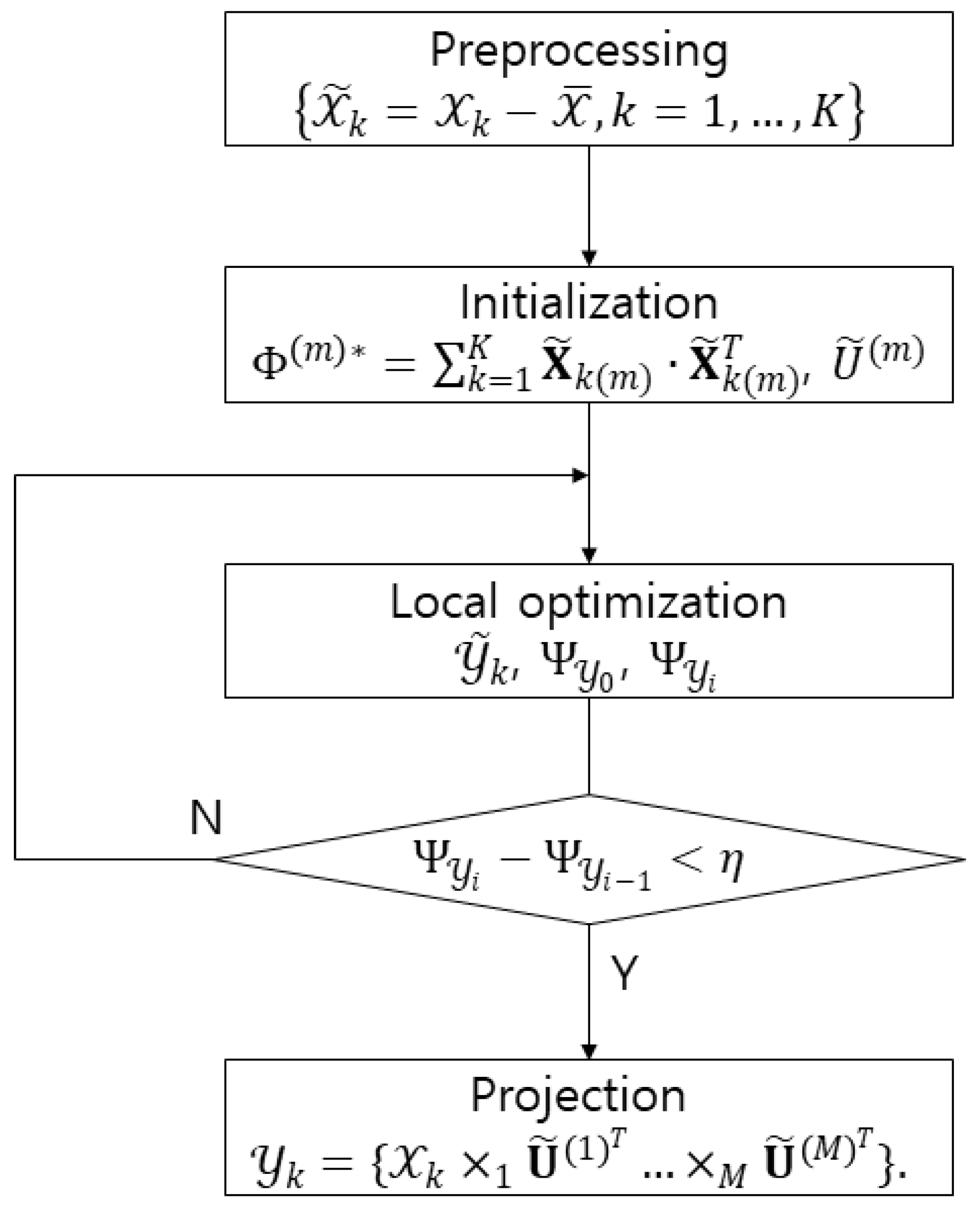
Assume that $\left\{{\mathcal{A}}_k,k=1,\dots ,K\right\}$ are K tensors in ${ℝ}^{I_1}\otimes {ℝ}^{I_2}\dots \otimes {ℝ}^{I_M}$. The entire scatter matrix of these tensors is written as ${\mathsf{\Psi }}_{\mathcal{A}}={\displaystyle \sum }_{k=1}^K\parallel {\mathcal{A}}_k-\overline{\mathcal{A}}{\parallel }_F^2$, where $\overline{\mathcal{A}}$ is the average tensor, computed as $\overline{\mathcal{A}}=\frac{1}{K}{\displaystyle \sum }_{k=1}^K{\mathcal{A}}_k$. The m-mode entire scatter matrix of these tensors is then written as: $S_{T_{\mathcal{A}}}^{\left(m\right)}={\displaystyle \sum }_{k=1}^K\left(A_{k\left(m\right)}-{\overline{A}}_{\left(m\right)}\right){\left(A_{k\left(m\right)}-{\overline{A}}_{\left(m\right)}\right)}^T$, where $A_{k\left(m\right)}$ is the m-mode spread matrix of ${\mathcal{A}}_k$. The following definition are generated by the words above to solve the problem: K tensors $\left\{{\mathcal{X}}_1, {\mathcal{X}}_2, \dots , {\mathcal{X}}_K\right\}$ can be used for training. Each tensor ${\mathcal{X}}_K\in {ℝ}^{I_1\times I_2\times \dots \times I_M}$ sets values in a tensor space ${ℝ}^{I_1}\otimes {ℝ}^{I_2}\dots \otimes {ℝ}^{I_M}$, where $I_m$ is the m-mode dimensional tensor. The MPCA is a multilinear projection of $\{{\tilde{U}}^{\left(m\right)}\in {ℝ}^{I_m\times P_m},m=1,\dots ,M\}$, mapping a high dimensional tensor space of ${ℝ}^{I_1}\otimes {ℝ}^{I_2}\dots \otimes {ℝ}^{I_M}$ to a low dimensional subspace of ${ℝ}^{P_1}\otimes {ℝ}^{P_2}\dots \otimes {ℝ}^{P_M}$ (with $P_m<I_m,\mathrm{for}m=1,\dots ,M):{\mathcal{Y}}_k={\mathcal{X}}_k{\times }_1{\tilde{U}}^{{\left(1\right)}^T}{\times }_2{\tilde{U}}^{{\left(2\right)}^T}\dots {\times }_M{\tilde{U}}^{{\left(M\right)}^T}, k=1,\dots ,K,$ such that most of the variations presented in the original tensor are obtained by $\left\{{\mathcal{Y}}_k\in {ℝ}^{P_1}\otimes {ℝ}^{P_2}\dots \otimes {ℝ}^{P_M}, k=1,\dots ,K\right\}$, assuming that the entire tensor scatter measures these variations. That is, the MPCA is performed by obtaining the N projection matrices $\left\{{\tilde{U}}^{\left(m\right)}\in {ℝ}^{I_m\times P_m},m=1,\dots ,M\right\}$ that make the entire tensor scatter ${\mathsf{\Psi }}_{\mathcal{Y}}$ become large. The flowchart of MPCA is described in Figure 1 and Figure 2 shows the process of multilinear projection [27,36]:

$$\left\{{\tilde{U}}^{\left(m\right)},m=1,\dots ,M\right\}=\arg ma{x}_{{\tilde{U}}^{\left(1\right)},{\tilde{U}}^{\left(2\right)},\dots ,{\tilde{U}}^{\left(M\right)}}{\mathsf{\Psi }}_{\mathcal{Y}}$$

(1)

2.2. Multilinear Linear Discriminant Analysis (MLDA)

The LDA looks for a straight line after projecting the data on a specific axis to separate the two classes [27]. The straight lines separating the two classes after the projection make the centers of the two classes away from each other, and make each variance small. $y$ is a one-dimensional vector where a vector x of p-dimension is projected on vector $w$. For $C_1$ class with $N_1$ data and $C_2$ class with $N_2$ data, the center vector of each class is $m_1$ and $m_2$:

$$y={\overrightarrow{w}}^T\overrightarrow{x}$$

(2)

$$m_1=\frac{1}{N_1}{{\displaystyle \sum }}_{n\in C_1}{x}_n$$

(3)

$$m_2=\frac{1}{N_2}{{\displaystyle \sum }}_{n\in C_2}{x}_n$$

(4)

In order to calculate the vector $w$ separating the centers of the two classes after projection, the relation between each center and $w$ is the same as below:

$$m_2-m_1=w^T\left(m_2-m_1\right)$$

(5)

$$m_k=w^T{m}_k$$

(6)

When the projection is performed, the closer the data is to the center of each class in order to reduce the variance, the better. The variance after projection is written as follows:

$$s_k^2={{\displaystyle \sum }}_{n\in C_k}{\left(y_n-m_k\right)}^2.$$

(7)

The objective function maximizing the distance between centers and minimizing each variance is as follows:

$$J\left(w\right)=\frac{{\left(m_1-m_2\right)}^2}{s_1^2+s_2^2}=\frac{w^T{S}_{B}w}{w^T{S}_{W}w}$$

(8)

$$S_B=\left(m_1-m_2\right){\left(m_1-m_2\right)}^T$$

(9)

$$S_W={\displaystyle \sum }_{n\in C_1}\left(x_n-m_1\right){\left(x_n-m_1\right)}^T+{\displaystyle \sum }_{n\in C_2}\left(x_n-m_2\right){\left(x_n-m_2\right)}^T$$

(10)

The objective function $J\left(w\right)$ becomes the largest when its derivative value for $w$ is 0.

$$(w^T{S}_{B}w)S_{W}w=(w^T{S}_{W}w)S_{B}w$$

(11)

The equation turns $AX=\lambda X$ because the parentheses are scalars. A new axis of $w$ is an eigenvector of $S_B^{-1}{S}_W$:

$$S_{W}w=\lambda S_{B}w$$

(12)

$$S_B^{-1}{S}_{W}w=\lambda w$$

(13)

$S_B$ and $S_W$ are the variances of the mean and variance of the data, respectively. The axis of $w$ could be obtained by eigendecomposition. The Fisher ECG method is that PCA is first used as a pre-processing step to remove the null space of $S_w$, and then LDA is performed in the lower-dimensional PCA subspace using ECG signals [37,38,39]. Figure 3 shows the process of multilinear discriminant analysis.

2.3. Comparison Multilinear Subspace Learning with Linear Subspace Learning

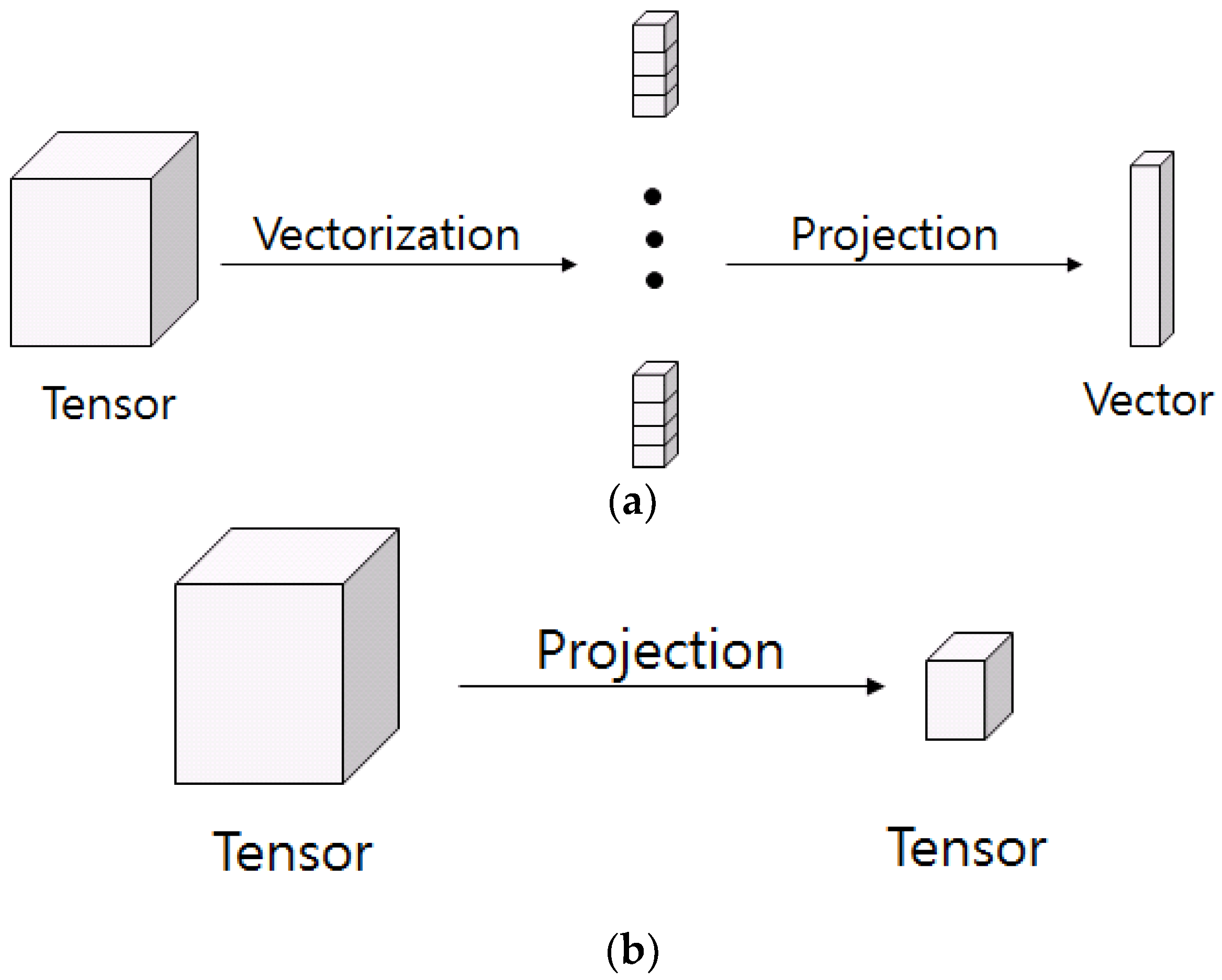
Figure 4 shows comparison of multilinear subspace learning. Traditional LSL methods include independent component analysis (ICA), PCA, LDA, and they receive vectors as inputs. To apply a two-dimensional or higher tensor to an LSL, such as an image or a video, the tensor must be rearranged in one dimension. LSL causes two disadvantages while vectorizing a high dimensional tensor to a one-dimensional tensor:

• Vectorization of LSL destroys the structural correlations of the original data, and that yields poor feature extraction.
• When a high dimensional tensor such as a video is rearranged into a one dimensional vector, the dimension of the one-dimensional tensor becomes very large. Analyzing a high dimensional vector results in a small sample size problem where the parameters to be estimated are larger than the number of data for training and results in high computing loads.

MSL maps high dimensional input tensor to low dimensional tensor with maintaining its structural information. Linear mapping requires the input to be rearranged as a vector, but multilinear mapping allows feature extraction without rearrangement. Linear mapping in high dimensional tensors requires many parameters, but multilinear mapping requires very few parameters. Linear mapping can extract various features with many parameters, but multilinear mapping extracts more compact features. This provides the following three advantages [40]:

• The input form of the tensor is preserved as the original shape.
• It is possible to extract more compact and useful features than LSL. MSL is less severe than LSL in the problem that the dimension of the data is much larger than the number of data that is required for training.
• High dimensional tensors can be efficiently processed in a lower dimension than in the linear method.

3. ECG Biometrics Based on Multilinear Subspace Learning

3.1. Preprocessing

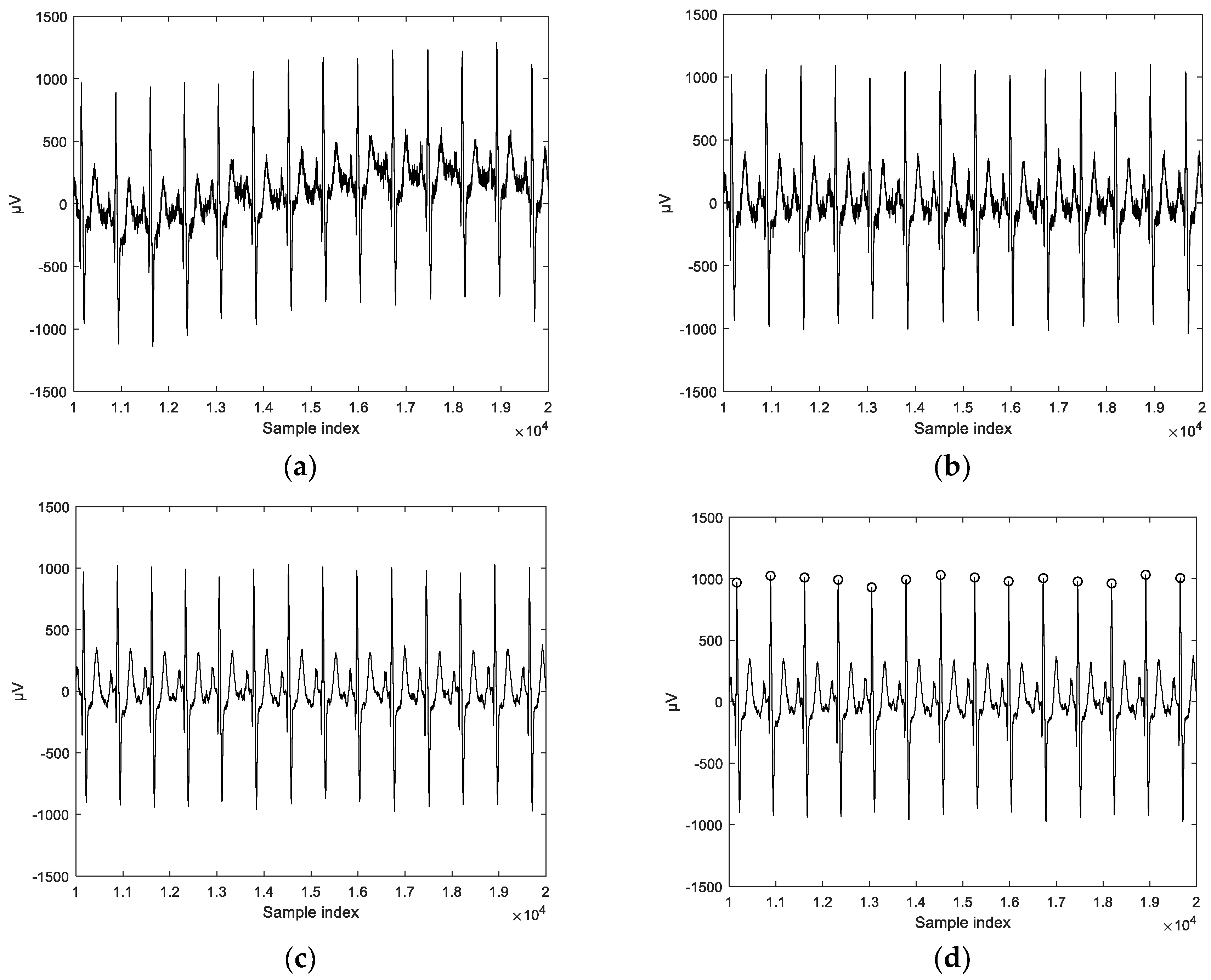
The original signal as shown in Figure 5a contains both high- and low-frequency noise components [41]. Therefore, the signal is normalized by subtracting the original signal from the convolutional signal with a mean filter of size 500, and the normalized signal shown in Figure 5b is convolved with a mean filter of size 10 to remove spikes. Next, 600 frames back and forth in the spike-removed signal of Figure 5c are removed to obtain a valid signal. Then, R peaks are detected in the ECG signal, and 392 frames back and forth are separated from the R peaks to obtain 784 frames. Only the I-lead is used for this study [42]. Figure 5d shows the detected peaks.

3.2. ECG Biometrics Based on Multilinear EigenECG (MEECG)

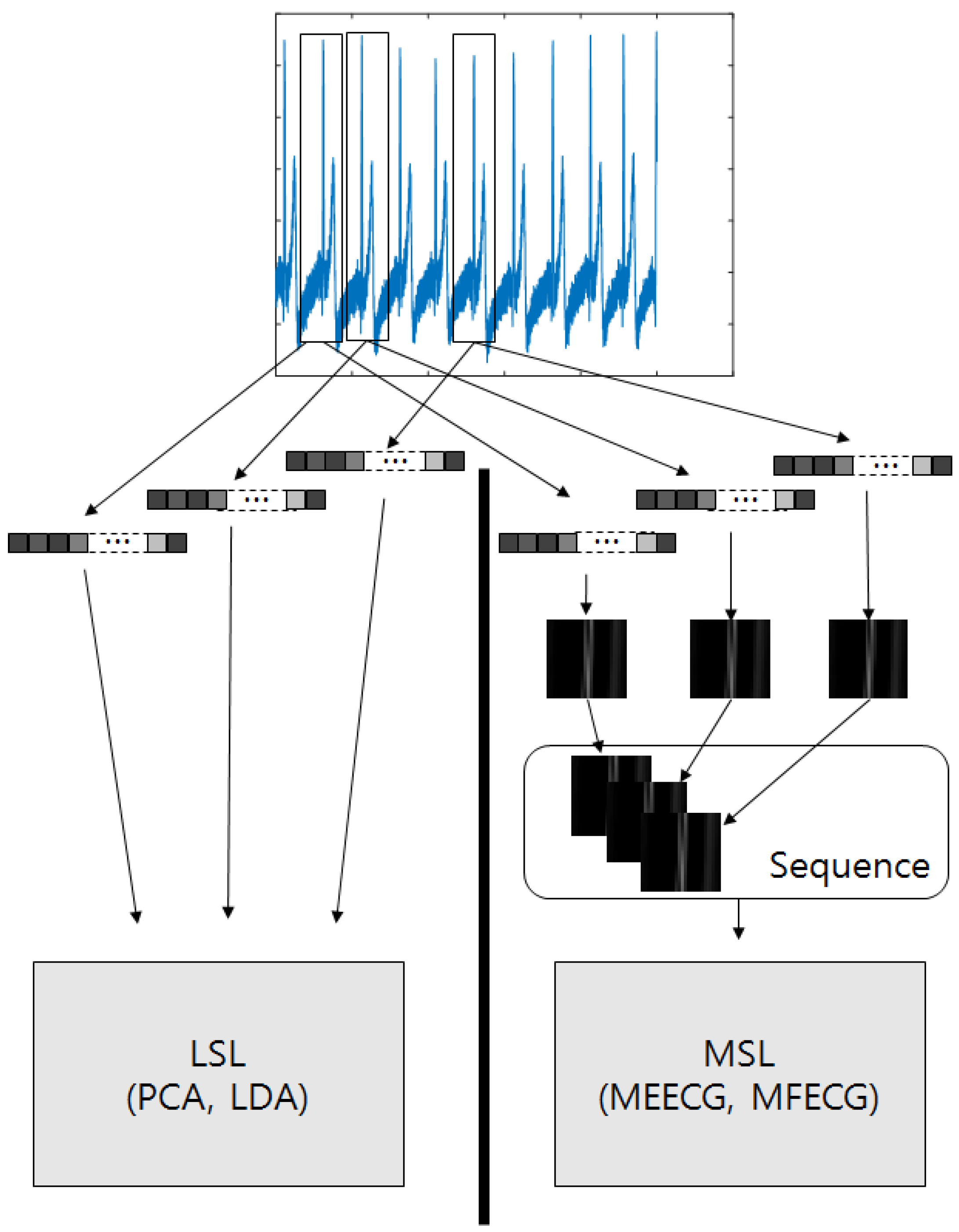
In the most active area, three-dimensional information, such as a 3D object [29], hyperspectral cube [30], or gait video sequence [31] with three modes following the x-axis, y-axis, and z-axis, a third-order tensor has been noted as an important point study [32,33,34]. Individual identification using ECG signals can be also considered as multilinear tensor spaces with temporal dimensions. However, the use of ECG signals is not commonly considered for a multidimensional tensor or for extracting features with multilinear projections. An ECG is normally gathered continuously as serial data. By applying it to a tensor, the input can include sequential information. Thus, tensor-based sequential input with the variant noisy ECG signals could be effectively classified. An ECG signal, a vector, is reshaped to 3D as a tensor. First, a vector is divided into several sub-vectors with regular sizes in a regular sequence, and the vector becomes a 2D tensor by stacking the sub-vectors. Second, sequential 2D tensors from ECG signals are reshaped to a 3D tensor by stacking following the temporal axis. The MPCA-based ECG is defined as a MEECG in this paper. Figure 6 shows the input shapes of LSL and MSL on the ECG signal.

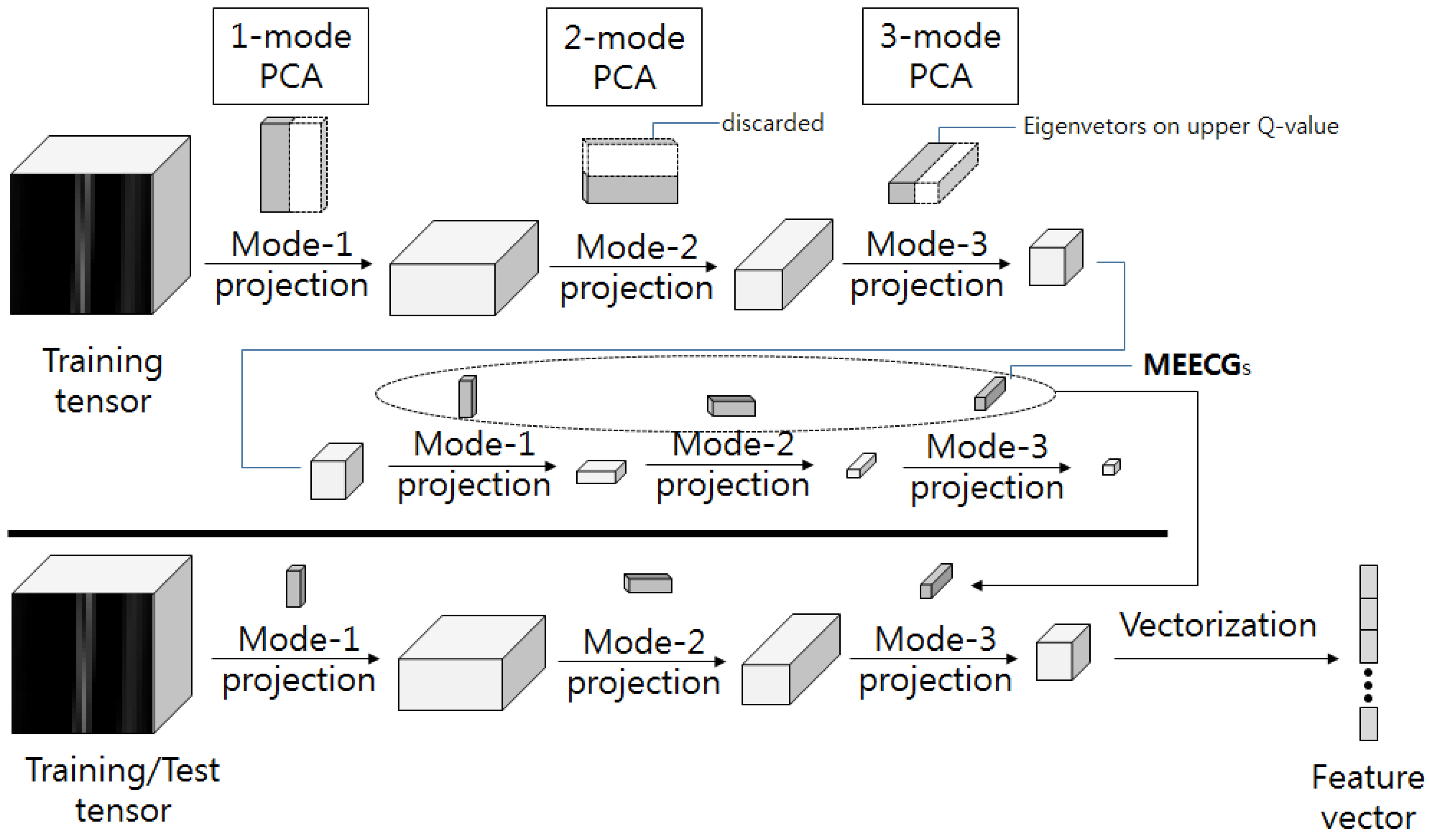
For the training data, the ECG signals are reshaped into a 3D tensor and then input to the MEECG. Each 3D tensor is subtracted by the mean of all training data, and the covariance matrix is obtained for each mode. The eigenvalues and eigenvectors are obtained by the covariance matrix and sorted in descending order to obtain the number of eigenvectors, including the upper percentage of variation kept in each mode (Q-value) on the accumulated eigenvalue. The remaining eigenvectors are discarded and features are extracted by projection with the eigenvectors of the upper Q-value in each mode. The covariance matrix is obtained for each extracted feature again, eigenvectors and eigenvalues are obtained by the covariance matrix of the extracted feature, and the eigenvectors for the final projections are obtained by sorting in descending order, resulting in the MEECGs. The MEECG accepts a 3D tensor as input, and yields a 3D tensor as output from the training data. This output of a 3D tensor becomes a feature vector through vectorization. Figure 7 shows the course of MEECG feature extraction [27].

3.3. ECG Biometrics Based on Multilinear Fisher ECG (MFECG)

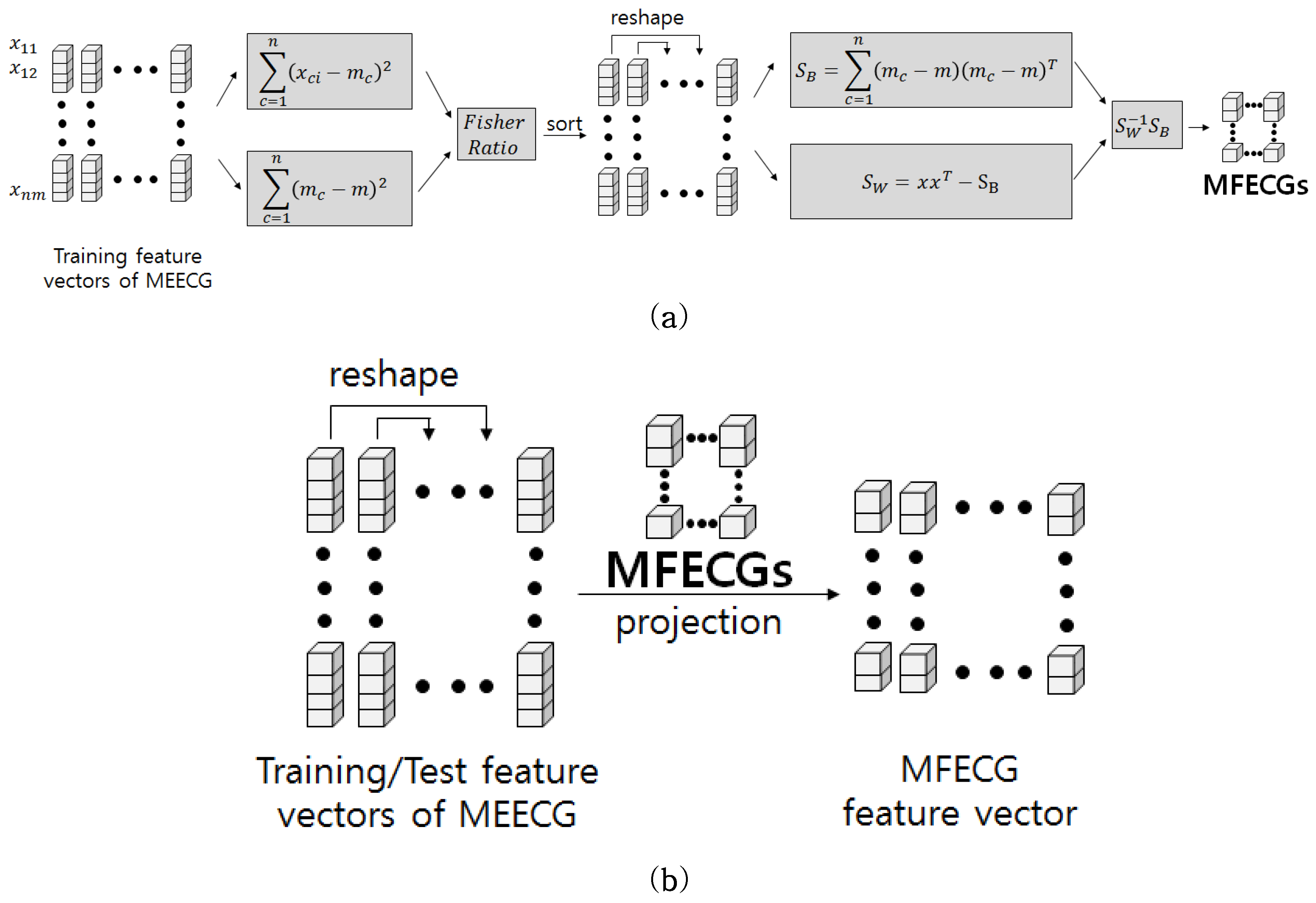
The MLDA-based ECG is defined as a MFECG in this paper. After constructing the feature vector using MEECG, the entire mean and means of each class are calculated. Using the means of each class, the variances indicating the spread of the data in each class are obtained, and the within-variance is the sum of the values. In addition, the variance between the entire mean and the means of each class are obtained, and the values are added together to obtain the between-variance. The Fisher ratio is obtained by dividing the between-variance by the within-variance, and it is sorted in descending order to reshape the feature vectors in descending order by a Fisher ratio, because the larger the Fisher ratio value, the better the feature vector. The entire mean and means of each class are obtained from the sorted feature vectors. The difference vector between the means of each class and entire mean are obtained. The covariance matrix is calculated from the difference vector, and $S_b$ is the sum of the values. $S_W$ is obtained by subtracting the covariance of each class from the entire covariance for the training data, and eigenvalues and eigenvectors are calculated from the $inv\left(S_w\right)*S_b$ matrix to yield the MFECG data. Finally, the MFECG feature vectors can be obtained by projecting the MEECG feature vectors for training and testing with these MFECG results. Figure 8 shows the course of MFECG feature extraction [27,37,38,39].

3.4. Similarity Measures

Individual identification using the ECG signal needs to classify similar signals, because humans have similar ECG signals to each other. Conventionally, to identify individuals using ECG signals, features based on fiducial points were successfully used and were defined as amplitudes and distances. There are several methods to measure similarity. Herein, three distance measures are considered: the Manhattan distance ($d_{L1}$), Euclidean distance ($d_{L2}$), and cosine similarity ($d_{Cos}$). The Manhattan and Euclidean distances are defined as the subtraction between two vectors. Cosine similarity (angle distance, AD) measures the angle between two vectors:

$$d_{L1}\left(x_t,x_v\right)={{\displaystyle \sum }}^{\text{}}\left|x_t-x_v\right|,$$

(14)

$$d_{L2}\left(x_t,x_v\right)=\sqrt{{{\displaystyle \sum }}^{\text{}}{\left(x_t-x_v\right)}^2},$$

(15)

$$d_{Cos}\left(x_t,x_v\right)=\frac{x_t{x}_v^T}{\parallel x_t\parallel \parallel x_v\parallel },$$

(16)

where $\parallel ·\parallel$ denotes the Euclidean distance, $x_t$ and $x_v$ are vector spaces with a fixed Cartesian coordinate system, and ${\mathsf{\Sigma }}^{-1}$ is the inverse matrix of the group covariances of the class [43,44,45].

3.5. Evaluation

The evaluation of individual identification is based on the notion of the numbers of correct classification (CC) and wrong classification (WC). Based on the individual identification results, the accuracy has been defined as follows [46,47]:

$$Accuracy= \frac{CC}{CC + WC }$$

(17)

3.6. Comparison of Correlation by Reshaping

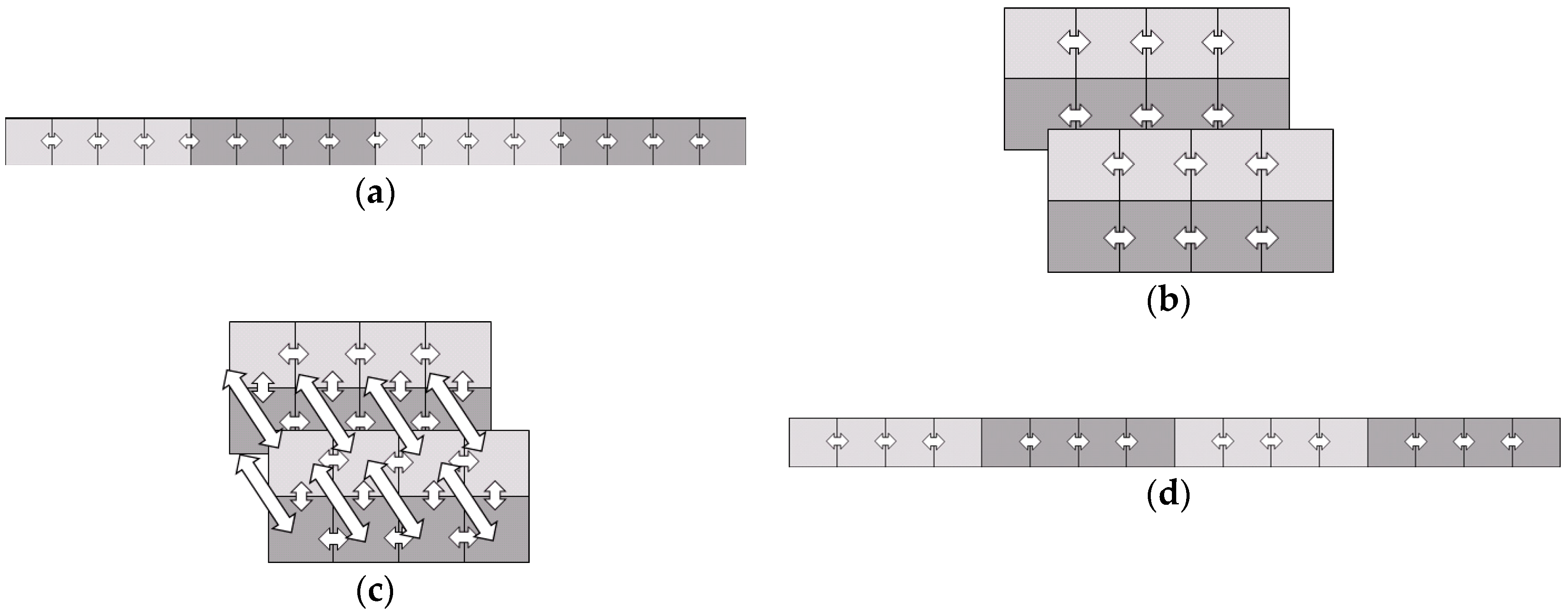
LSL must perform vectorization in one dimension to analyze more than data of more than two dimensions. This vectorization reduces a certain level of correlation among the data in the original dimensionality. In other words, reshaping the data reduces the level of correlation in the original data. In this study, a one-dimensional vector is reshaped to a 3D tensor to apply a one-dimensional ECG signal to MSL. In the process, the correlation that the data have is reduced. If the one-dimensional ECG signal is applied to the MSL, the correlation is reduced through reshaping, and the advantage of the MSL is attenuated. However, assuming that there is only correlation between neighboring data, there is a difference in the amount of correlation that must be reduced in order to reshape a vector to a higher dimension from that of reshaping a tensor of higher dimension to a vector. Figure 9 shows a comparison of correlation by reshaping. As shown in Figure 9a, the 1D vector had 15 correlations (the number of arrows), but reshaping it to a 3D tensor, as shown in Figure 9b, maintained 12 correlations. On the other hand, as shown in Figure 9c, the 3D tensor had 28 correlations before reshaping. However, when reshaping it to a 1D vector, as shown in Figure 9d, only 12 correlations remained. That is, in the case of an ECG signal, to reshape a tensor from a high dimension to a low dimension reduces correlation, but to reshape a tensor from a low dimension to a high dimension retains most of the correlations. Furthermore, as shown in Figure 10, when reshaping from a low dimension to a high dimension, there is the possibility that new correlations can be generated. In this paper, we apply a 1D ECG signal to MSL, to better conserve the correlations and to analyze the new correlations generated from reshaping the 1D ECG signal to a 2D signal and from 2D to 3D as sequential information.

4. Experimental Results

Linear subspace learning like PCA and LDA requires the reordering of high dimensional data as a vector, destroying the structural correlations of the original data. Furthermore, there is a problem that the dimension of data is much larger than the number of data required for training. The latest multilinear subspace learning (MSL) preserves the geometric information of the original data by extracting and mapping features without deformation of tensor structure, and it is possible to deal with large tensors efficiently because the problem that the dimension of data can be larger than the number of data for training is alleviated. Here, MPCA and MLDA are considered to be MSL [27]. To apply 1D ECG signals to MSL, it is necessary to reshape the vector from a low dimension to a high dimension. This also reduces some correlations, but few correlations are affected in the ECG signal, and there is a possibility that new correlations can be generated. The PTB-ECG and the CU-ECG databases are used for this study. PTB-ECG is a universally well-known database for ECG signals, and CU-ECG is a database of ECG signals built specifically for this study. The MPCA-based ECG is MEECG, and the MLDA-based ECG is MFECG in this paper.

4.1. PTB-ECG Database

This ECG data was acquired from the Physikalisch-Technische Bundesanstalt (PTB), the National Metrology Institute of Germany to automatically diagnose with a computer and is a large database with 27,000 recordings. The ECG signals were acquired in a sitting position in a resting state by many people. Electrocardiogram signals were collected from healthy people and from people with heart disease. The ECG signals were obtained from 290 people consisting of men and women of different ages, including information from 15 leads. The 15 leads consisted of 12 standard leads (I, II, III, aVR, aVL, aVF, V1, V2, V3, V4, V5 and V6) and three Frank leads (Vx, Vy, and Vz). The ECG signal was measured at 1000 samples/s, and it was measured with 16 bit accuracy over a voltage range of ±16.384 mV [35]. The ECG signals varied in the number of recordings for each person, and most people were recorded two or three times, and the recording length varied from 23 s to 2 min. The difference of the measured time between the ECG records of the same person was an average of 500 days [48].

4.2. CU-ECG Database

CU-ECG is a database of ECG signals directly built for this study. This database includes data of 100 subjects: 89 males and 11 females of ages ranging from 23 to 34 years old. The ECG signals were measured 60 times per subject while the subjects were comfortably positioned in a chair; 10 s were recorded at a time, and the type of ECG was lead-I. The sampling rate of the ECG signal was 500 kHz. The developed device measuring ECG signals was composed of a wet-corrosion electrode, Atmega8 and Keysight MSO9104.

The base board of the developed device using Atmega8 and its diagram are described in Figure 11. The base board was configured to receive a voltage of 6–12 V and to output a voltage of 5 V, and the LD1117 was built in for a 5 V constant voltage output. The power supply of the base board was mainly composed of two types of power sources. One supplied 5 V for the microcontroller (MCU) and other parts and the other supplied 5 V and −5 V for BIO-AMPs. LM2664 was used as a chip that converts 5 V to −5 V for negative power input to the analog terminal. The A/D (Analog to Digital) converter of Atmega8 can generate a 10-b resolution and can use 0–5 inputs through the MCU as 0–1024. In other words, the input value of the voltage can be considered by dividing by 5 mV units, and there are four such A/D input terminals. It is manufactured to enable external RS-232 communication and USB (Universal Serial Bus) communication using UART1 inside Atmega8. USB communication is programmed in the same way as ordinary serial communication, but it is made to convert data using a USB-to-serial chip. The communication speed is 9600–115,200 bps, but the demo program is ported at 115,200 bps. The input and output terminals consist of one input switch and four output LEDs (Light-Emitting Diodes). The demo program is ported to allow four LEDs to toggle simultaneously during device operation.

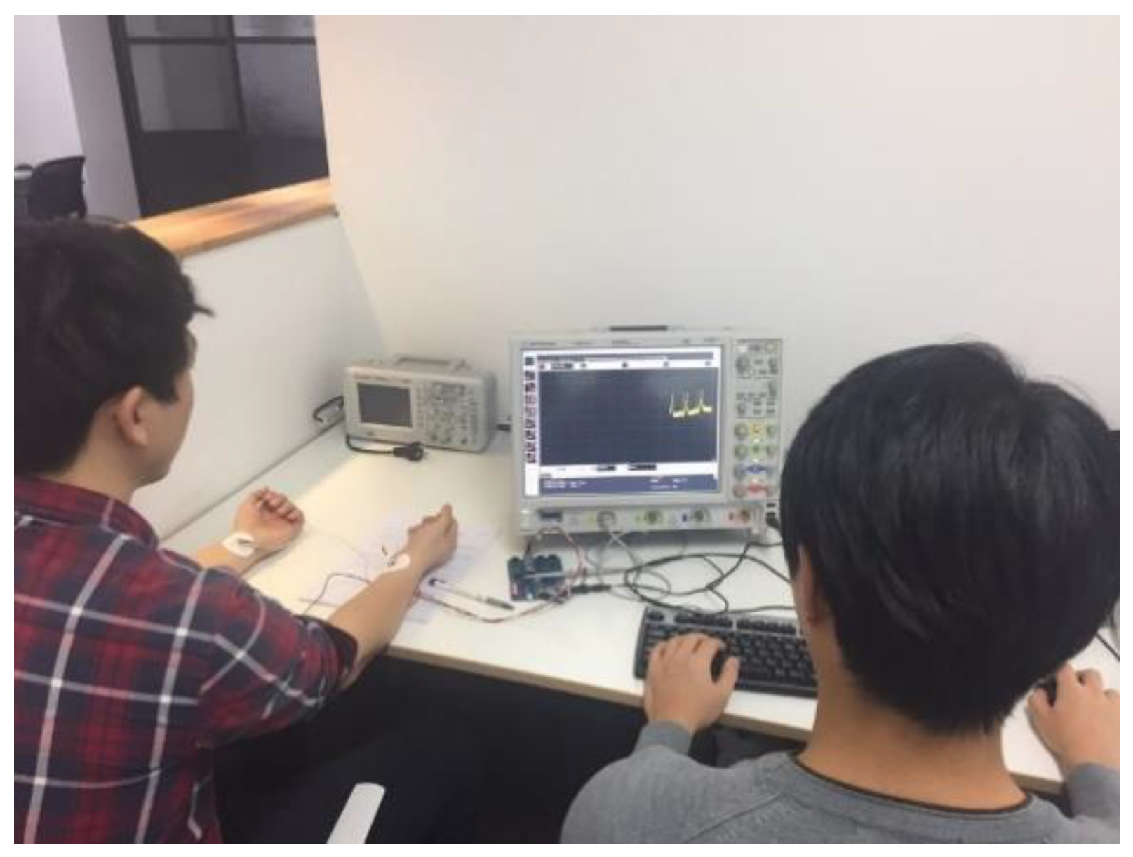
The preamplifier section for measuring general bio-signals consists of a differential amplifier section. The potential difference input from the positive and negative ends of the electrode to be measured is checked and the bio-electrical potential generated between them is measured. In the preamplifier section, all types of body signals were actually measured. The needed signals input from the preamplifier became clear by rectifying and amplifying the band of the part in which the actual bio-signal was present. The specific frequency band or amplification of the desired bio-signals could be adjusted. However, this device was made by using minimum amplification with a wide bandwidth in order to measure all the ECG, electroencephalogram (EEG), and electromyography (EMG) signals, and it filtered them precisely using digital filters through a personal computer. Electricity for general use flows at a frequency of 60 Hz in our country. This affects analog measuring equipment and medical equipment. For this reason, a band-stop filter was applied to the BIO-AMP to minimize the noise by setting the frequency value to be slightly wider at around 60 Hz. The low-pass filter with a cut-off frequency of 150 Hz was designed to eliminate noise generated at high frequencies and to measure ECG and EEG waves below 150 Hz without problems. The voltage offset was adjusted using the adder circuit in order to input the reference value by converting the final output signal, which has a value of −5 V to 5 V, to the value of the MCU terminal, which is 0 V to 5 V. Figure 12 shows the measurement environment of ECG signals.

4.3. Experimental Results

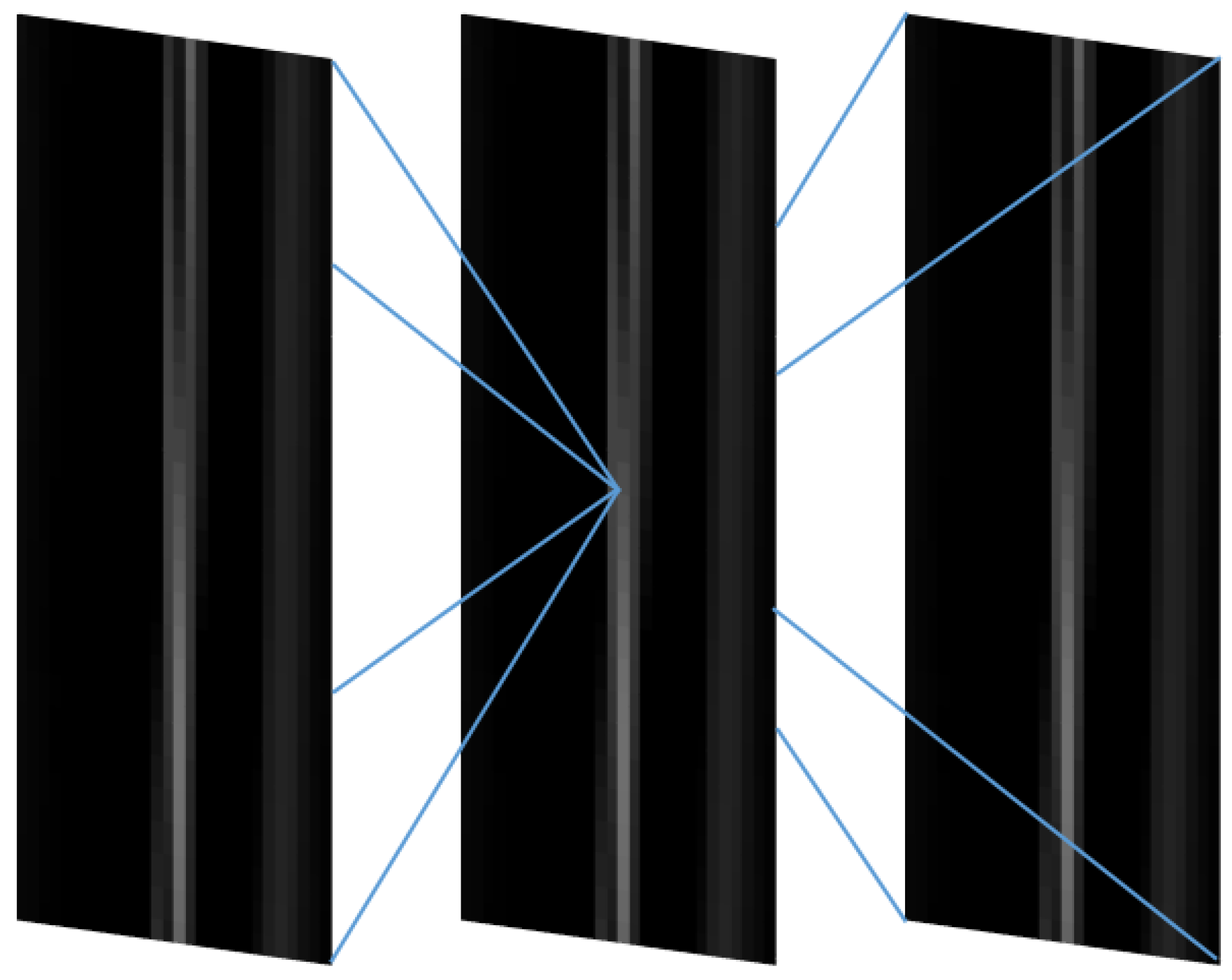
The computer specification used in the experiment is Intel(R) Core(TM) i5-4440 CPU at 3.10 GHz, NVIDIA GeForce GT 630 and 8 GB RAM. In this study, individual identification with ECG was performed by preprocessing the input ECG signal only with I-lead, and when the R peak points were detected, 784 frames of data were acquired by 392 frames back and forth, based on the R peak point. R peak points were detected for all recordings, and the numbers of R peak points detected for each class were obtained. To construct an equal amount of data for each class, classes that had a very small number of R peak points were excluded, and the number of samples of all classes was adjusted to the smallest number of R peak points among the remaining classes. The preprocessed signals were then rearranged symmetrically to 3D tensors. The lengths of row and column were same as each other to construct a symmetric structure. The 784 frames extracted from ECG signal were directly transformed to a 28 × 28 image. After that, the images of three signals were lined up following the temporal axis. These symmetric tensors entered MPCA for feature extraction. Then classification was performed by using three distance similarities. Figure 13 shows the symmetric tensor.

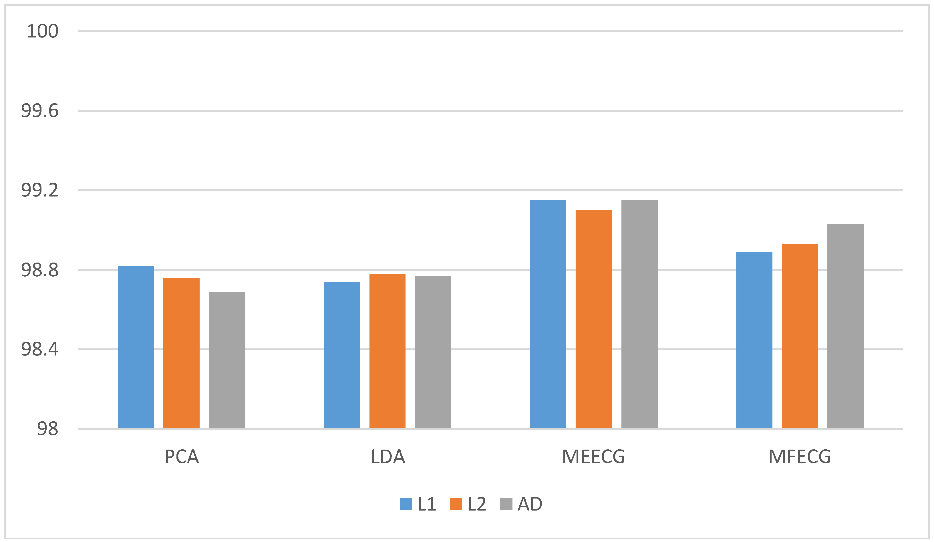
In the case of PTB-ECG, the 79 classes that have a very small number of R peak points were excluded among 290 classes. The common maximum number of R peak points among the rest of the classes was 120. That is, the data was composed of 120 samples per class. The constructed data size is 784 × 25,320 (120 samples/class × 211 classes); the row indicates the dimension of the data and the column indicates the number of samples. The preprocessed signals was vectors. That means that LSL (PCA and LDA) could directly accept them as input, and the ratio of training was 50%. The sizes of the data for training and test were 784 × 12,660 each. To make the input to MSL (MEECG and MFECG), the vectors were reshaped to 2D with rows and columns of the same size, and the vectors became 2D tensors of size 28 × 28 × 25,320. Then, the sequential 2D tensors were reshaped to 3D tensors by stacking following the temporal axis. The size of the 3D tensor was 28 × 28 × 3 × 8440 by three stacked 2D tensors, and the ratio of training was 50%. The sizes of data for training and test were 28 × 28 × 3 × 4220 each.

Table 1. Accuracies of PCA on Physikalisch-Technische Bundesanstalt (PTB)-ECG.

PCA Dimension	L1 (%)	L2 (%)	Angle distance (AD) (%)
10	98.70	98.71	98.51
20	98.74	98.76	98.69
30	98.82	98.74	98.68
40	98.73	98.72	98.68
50	98.72	98.72	98.66
60	98.68	98.72	98.67
70	98.68	98.72	98.67
80	98.68	98.72	98.67
90	98.68	98.72	98.67
100	98.67	98.72	98.67

,

Table 2. Accuracies of LDA on PTB-ECG.

LDA Dimension	PCA Dimension	L1 (%)	L2 (%)	AD (%)
21	11	98.70	98.70	98.64
	12	98.72	98.77	98.66
	13	98.73	98.72	98.64
	14	98.72	98.71	98.67
	15	98.71	98.74	98.69
	16	98.70	98.76	98.70
	17	98.74	98.74	98.71
	18	98.72	98.78	98.77
	19	98.70	98.76	98.71
	20	98.63	98.77	98.74

,

Table 3. Accuracies of MEECG on PTB-ECG.

MEECG Dimension	L1 (%)	L2 (%)	AD (%)
10	98.91	98.65	98.25
20	99.10	99.03	98.82
30	99.15	99.10	99.15
40	99.05	98.98	99.08
50	99.05	98.98	99.12
60	98.96	98.86	98.98
70	98.96	98.74	98.82
80	98.96	98.72	98.79
90	98.96	98.72	98.74
100	98.74	98.65	98.67

and

Table 4. Accuracies of MFECG on PTB-ECG.

MFECG Dimension	L1 (%)	L2 (%)	AD (%)
10	98.72	98.89	98.77
20	98.89	98.93	98.98
30	98.86	98.93	99.00
40	98.82	98.91	99.03
50	98.82	98.89	99.00
60	98.82	98.86	99.03
70	98.84	98.84	99.03
80	98.70	98.82	98.91

show the accuracies of PCA, LDA, MEECG, and MFECG on the PTB-ECG database, respectively. The PCA dimension in LDA was set to 21, which made the Q-value 97%. The dimensions of PCA, MEECG, and MFECG varied from 10 to 100 with a step size of 10. The best dimensions were selected as the best accuracies. In the case of PTB-ECG, the highest accuracies of PCA in each distance were 98.82% of L1, 98.76% of L2, and 98.69% of AD; the highest accuracies of LDA in each distance were 98.74% of L1, 98.78% of L2, and 98.77% of AD; the highest accuracies of MEECG in each distance were 99.15% of L1, 99.10% of L2, and 99.15% of AD; and the highest accuracies of MFECG in each distance were 98.89% of L1, 98.93% of L2, and 99.03% of AD.

In the case of CU-ECG, subsampling was performed from 500 kHz to 1 kHz because the data is too big due to the high sampling rate for processing, and one class that has a very small number of R peak points was excluded among the 100 classes. The common maximum number of R peak points among the rest of the classes was 300. That is, the data was composed of 300 samples per class. The constructed data size was 784 × 29,700 (300 samples/class × 99 classes); the row indicates the dimension of the data and the column indicates the number of samples. The preprocessed signals are vectors. That means that LSL (PCA and LDA) could directly accept them as input, and the ratio of training is 50%. The sizes of data for training and test were 784 × 14,850 each. To make the input to MSL (MEECG and MFECG), the vectors were reshaped to 2D with rows and columns of the same size, and the vectors became 2D tensors of size 28 × 28 × 29,700. Then, the sequential 2D tensors were reshaped to 3D tensors by stacking following the temporal axis. The size of the 3D tensor was 28 × 28 × 3 × 9900 by three stacked 2D tensors, and the ratio of training was 50%. The sizes of data for training and test were 28 × 28 × 3 × 4950 each.

Table 5. Accuracies of PCA on Chosun University (CU)-ECG.

PCA Dimension	L1 (%)	L2 (%)	AD (%)
10	91.52	91.58	89.67
20	93.41	93.21	92.51
30	93.64	93.30	92.66
40	93.63	93.33	92.65
50	93.42	93.29	92.42
60	93.25	93.22	92.34
70	93.11	93.21	92.27
80	93.07	93.22	92.27
90	93.03	93.22	92.24
100	92.98	93.22	92.19

,

Table 6. Accuracies of LDA on CU-ECG.

LDA Dimension	PCA Dimension	L1 (%)	L2 (%)	AD (%)
19	9	91.86	91.89	90.70
	10	92.84	92.84	91.98
	11	93.16	93.18	92.65
	12	93.08	93.21	92.95
	13	93.23	93.30	93.02
	14	93.16	93.12	92.97
	15	93.19	93.14	92.96
	16	93.28	93.17	92.92
	17	93.14	93.16	92.88
	18	93.00	93.17	92.86

,

Table 7. Accuracies of MEECG on CU-ECG.

MEECG Dimension	L1 (%)	L2 (%)	AD (%)
10	93.84	93.45	91.43
20	95.92	95.68	94.65
30	95.62	95.07	94.14
40	94.73	94.34	93.45
50	94.26	94.02	93.07
60	94.20	93.90	92.89
70	94.10	93.96	92.87
80	94.00	93.96	92.69

and

Table 8. Accuracies of MFECG on CU-ECG.

MFECG Dimension	L1 (%)	L2 (%)	AD (%)
10	95.94	95.70	94.99
20	95.90	95.76	95.72
30	95.72	95.72	95.45
40	95.41	95.43	95.33
50	94.99	95.13	95.13
60	94.59	95.01	94.95
70	94.30	94.93	94.85
80	93.66	94.77	94.79

show the accuracies of PCA, LDA, MEECG, and MFECG on the CU-ECG database, respectively. The PCA dimension in LDA was set to 19, which made the Q-value 97%. The dimensions of PCA, MEECG, and MFECG varied from 10 to 100 with a step size of 10. The best dimensions were selected as the best accuracies. In the case of CU-ECG, the highest accuracies of PCA in each distance were 93.64% of L1, 93.33% of L2, and 92.66% of AD; the highest accuracies of LDA in each distance were 93.28% of L1, 93.30% of L2, and 93.02% of AD; the highest accuracies of MEECG in each distance were 95.92% of L1, 95.68% of L2, and 94.65% of AD; and the highest accuracies of MFECG in each distance were 95.94% of L1, 95.76% of L2, and 95.72% of AD.

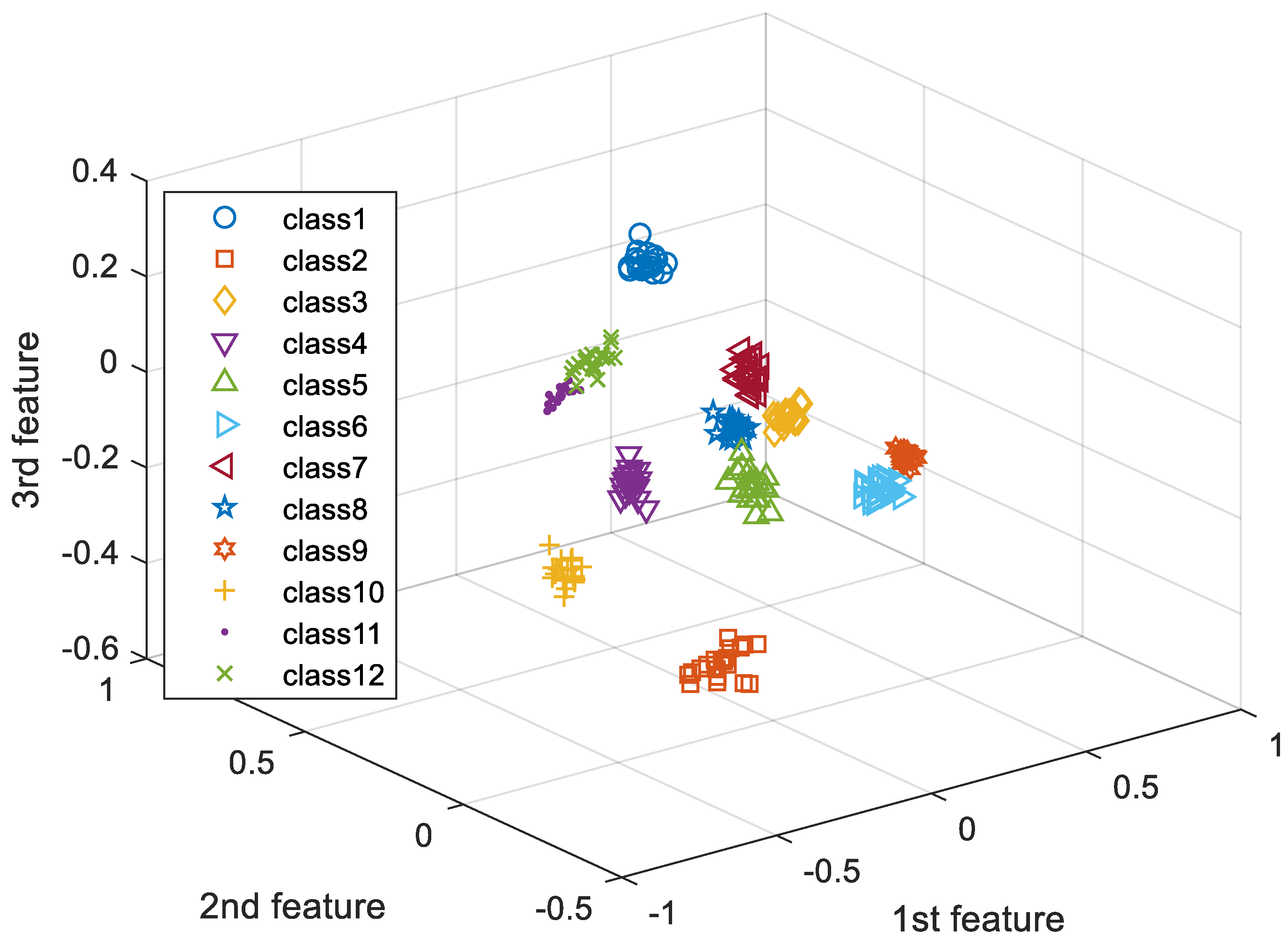
Figure 14 shows the comparison of the highest accuracies for each distance and method on PTB-ECG, and Figure 15 shows the same data on CU-ECG. In the case of PTB-ECG, the highest accuracies of MEECG in L1, L2, and AD were 0.33%, 0.34%, and 0.46% higher than the highest accuracies of PCA, and the highest accuracies of MFECG in L1, L2, and AD were 0.15%, 0.15%, and 0.26% higher than the highest accuracies of LDA, respectively. In the case of CU-ECG, the highest accuracies of MEECG in L1, L2, and AD were 2.28%, 2.35%, and 1.99% higher than the highest accuracies of PCA, and the highest accuracies of MFECG in L1, L2, and AD were 2.66%, 2.46%, and 2.70% higher than the highest accuracies of LDA, respectively. Figure 16 shows the MEECG feature space for 12 classes, and Figure 17 shows the MFECG feature space for 12 classes.

5. Conclusions

We present third-order tensor-based multilinear EigenECG and multilinear FisherECG for individual identification from the information of an electrocardiogram sensor. The vectorization of LSL destroys the structural correlations of the original data. However, the MSL preserves the geometric information of original data by extracting features without deformation of the tensor structure. Normally, reshaping from a high dimension to a low dimension reduces some correlations, but reshaping from a low dimension to a high dimension preserves most correlations. Moreover, there is a possibility that reshaping from a low dimension to a high dimension could generate new correlations. An ECG is normally gathered continuously as serial data. By applying it to a tensor, the input could arrange sequential information symmetrically in a tensor. Thus, tensor-based sequential input with the variant noisy ECG signals could be complementarily classified. Even if some parts among ECGs as sequential input are damaged, they can be complementary to each other. The databases of PTB-ECG and CU-ECG are used for this study. PTB-ECG is a well-known database for ECG signals, and the CU-ECG is a database of ECG signals built for this study. After preprocessing, the ECG signal is reshaped to a 3D tensor by stacking three ECG beats for sequence data for input to the MSL. The experiments are performed at distances of L1, L2, and AD. The MSL (MEECG and MFECG) has better performance than LSL (PCA and LDA) when individual identification is performed using ECG signals. For further research, we will study a method to build a more meaningful tensor for classification.

References

1. Wang, H.; Hu, J.; Deng, W. Compressing fisher vector for robust face recognition. IEEE Access. 2017, 5, 23157–23165. [Google Scholar] [CrossRef]
2. Jain, A.K.; Arora, S.S.; Cao, K.; Best-Rowden, L.; Bhatnagar, A. Fingerprint recognition of young children. IEEE Trans. Inf. Forensics Secur. 2017, 12, 1505–1514. [Google Scholar] [CrossRef]
3. Nguyen, B.P.; Tay, W.L.; Chui, C.K. Robust biometric recognition from palm depth images for gloved hands. IEEE Trans. Hum.-Mach. Syst. 2015, 45, 799–804. [Google Scholar] [CrossRef]
4. Zhang, Y.; Juhola, M. On biometrics with eye movements. IEEE J. Biome Health Inform. 2017, 21, 1360–1366. [Google Scholar] [CrossRef] [PubMed]
5. Pokhriyal, N.; Tayal, K.; Nwogu, I.; Govindaraju, V. Cognitive-biometric recognition from language usage: A feasibility study. IEEE Trans. Inf. Forensics Secur. 2017, 12, 134–143. [Google Scholar] [CrossRef]
6. Boles, W.W. A security system based on human iris identification using wavelet transform. In Proceedings of the First International Conference on Conventional and Knowledge based Intelligent Electronics Systems, Adelaide, SA, Australia, 21–23 May 1997; pp. 533–541. [Google Scholar]
7. Choi, G.H.; Moon, H.M.; Pan, S.B. Biometrics system technology trends based on biosignal. J. Digit. Convers. 2017, 15, 381–391. [Google Scholar] [CrossRef]
8. Gahi, Y.; Lamrani, M.; Zoglat, A.; Guennoun, M.; Kapralos, B.; El-Khatib, K. Biometric identification system based on electrocardiogram data. In Proceedings of the New Technologies, Mobility and Security, Tangier, Morocco, 5–7 November 2008; pp. 1–4. [Google Scholar]
9. Kim, J.J.; Lee, S.M.; Ryu, G.S.; Lee, J.H.; Park, K.H. Hierarchical authentication algorithm using curvature based fiducial point extraction of ECG signals. J. Korea Multi Soc. 2017, 20, 465–473. [Google Scholar] [CrossRef]
10. Kim, J.K.; Lee, K.B.; Hong, S.G. ECG-based biometric authentication using random forest. J. Inst. Electron. Inf. Eng. 2017, 54, 100–105. [Google Scholar]
11. Lim, C.S. A study on the analysis of technology and service issues for wearable devices and future development direction. J. Korea Inst. Next Gener. Comput. 2017, 13, 81–89. [Google Scholar]
12. Lathauwer, L.D.; Moor, B.D.; Vandewalle, J. A multilinear singular value decomposition. SIAM J. Matrix Anal. Appl. 2000, 21, 1253–1278. [Google Scholar] [CrossRef]
13. Greub, W. Multilinear Algebra, 2nd ed.; Springer-Verlag: New York, NY, USA, 1978; pp. 1–296. ISBN 9780387902845. [Google Scholar]
14. Kolda, T.G.; Bader, B.W. Tensor decompositions and applications. Siam Rev. 2009, 51, 455–500. [Google Scholar] [CrossRef]
15. Howe, D.; Costanzo, M.; Fey, P.; Gojobori, T.; Hannick, L.; Hide, W.; Hill, D.P.; Kania, R.; Schaeffer, M.; Pierre, S.S.; et al. Big data: The future of biocuration. Nature 2008, 455, 47–50. [Google Scholar] [CrossRef] [PubMed]
16. Armbrust, M.; Fox, A.; Griffith, R.; Joseph, A.D.; Katz, R.; Konwinski, A.; Lee, G.H.; Patterson, D.; Babkin, A.; Stoica, I.; et al. A view of cloud computing. Commun. ACM 2010, 53, 50–58. [Google Scholar] [CrossRef]
17. Dean, J.; Ghemawat, S. MapReduce: Simplified data processing on large clusters. Commun. ACM 2008, 51, 107–113. [Google Scholar] [CrossRef]
18. Shakhnarovich, G.; Moghaddam, B. Face recognition in subspaces. In Handbook of Face Recognition; Li, S.Z., Jain, A.K., Eds.; Springer-Verlag: New York, NY, USA, 2004; pp. 141–168. ISBN 038740595X. [Google Scholar]
19. Zhang, J.; Li, S.Z.; Wang, J. Manifold learning and applications in recognition. In Intelligent Multimedia Processing with Soft Computing; Tan, Y.P., Yap, K.H., Wang, L., Eds.; Springer-Verlag: Berlin, Germany, 2004; Volume 168, pp. 281–300. ISBN 354023053X. [Google Scholar]
20. Burges, C.J.C. Dimension reduction: A guided tour. Found. Trends Mach. Learn. 2010, 2, 275–365. [Google Scholar] [CrossRef]
21. Law, M.H.C.; Jain, A.K. Incremental nonlinear dimensionality reduction by manifold learning. IEEE Trans. Pattern Anal. Mach. Int. 2006, 28, 377–391. [Google Scholar] [CrossRef] [PubMed]
22. Jolliffe, I.T. Principal Component Analysis, 2nd ed.; Springer-Verlag: New York, NY, USA, 2002; pp. 1–488. ISBN 9780387954424. [Google Scholar]
23. Yang, J.; Zhang, D.; Frangi, A.F.; Yang, J. Two-dimensional PCA: A new approach to appearance-based face representation and recognition. IEEE Trans. Pattern Anal. Mach. Int. 2004, 26, 131–137. [Google Scholar] [CrossRef]
24. Ye, J.; Janardan, R.; Li, Q. GPCA: An efficient dimension reduction scheme for image compression and retrieval. In Proceedings of the Tenth ACM SIGKDD International Conference on Knowledge Discovery and Data Mining, Seattle, WA, USA, 22–25 August 2004; pp. 354–363. [Google Scholar]
25. Ye, J. Generalized low rank approximations of matrices. Mach. Learn. 2005, 61, 167–191. [Google Scholar] [CrossRef]
26. He, X.; Cai, D.; Niyogi, P. Tensor subspace analysis. Advances in Neural Information Processing Systems 18 (NIPS), Vancouver, BC, Canada, 5–8 December 2005; pp. 1–8. [Google Scholar]
27. Lu, H.; Plataniotis, K.N.; Venetsanopoulos, A.N. MPCA: Multilinear principal component analysis of tensor objects. IEEE Trans. Neural Netw. 2008, 19, 18–39. [Google Scholar] [PubMed]
28. Lu, H.; Plataniotis, K.N.; Venetsanopoulos, A.N. Multilinear Subspace Learning: Dimensionality Reduction of Multidimensional Data, 1st ed.; CRC Press: London, UK, 2013; pp. 1–296. ISBN 9781439857243. [Google Scholar]
29. Sahambi, H.S.; Khorasani, K. A neural-network appearance-based 3-D object recognition using independent component analysis. IEEE Trans. Neural Netw. 2003, 14, 138–149. [Google Scholar] [CrossRef] [PubMed]
30. Li, N.; Liu, C.; Pfeifer, N.; Yin, J.F.; Liao, Z.Y.; Zhou, Y. Tensor modeling based for airborne LiDAR data classification. In Proceedings of the Congress of 23rd ISPRS, Prague, Czech Republic, 12–19 July 2016; pp. 283–287. [Google Scholar]
31. Chen, J. Gait correlation analysis based human identification. Sci. World J. 2014, 2014, 1–8. [Google Scholar] [CrossRef] [PubMed]
32. Bowyer, K.W.; Chang, K.; Flynn, P. A survey of approaches and challenges in 3D and multi-modal 3D + 2D face recognition. Comput. Vis. Image Underst. 2006, 101, 1–15. [Google Scholar] [CrossRef]
33. Li, S.Z.; Zhao, C.; Zhu, X.; Lei, Z. Learning to fuse 3D+2D based face recognition at both feature and decision levels. In Proceedings of the IEEE International Workshop on Analysis and Modeling of Faces and Gestures, Beijing, China, 16 October 2005; pp. 44–45. [Google Scholar]
34. Colombo, A.; Cusano, C.; Schettini, R. 3D face detection using curvature analysis. Pattern Recognit. 2006, 39, 444–455. [Google Scholar] [CrossRef]
35. Goldberger, A.L.; Amaral, L.N.; Glass, L.; Hausdorff, J.M.; Ivanov, P.C.; Mark, R.G.; Mietus, J.E.; Moody, G.B.; Peng, C.K.; Stanley, H.E. PhysioBank, PhysioToolkit, and PhysioNet: Components of a new research resource for complex physiologic signals. Circulation 2000, 101, e215–e220. [Google Scholar] [CrossRef] [PubMed]
36. Wang, S.; Yang, X.; Zhang, Y.; Phillips, P.; Yang, J.; Yuan, T.F. Identification of green, oolong and black teas in China via wavelet packet entropy and fuzzy support vector machine. Entropy 2015, 17, 6663–6682. [Google Scholar] [CrossRef]
37. Belhumeur, P.; Hespanha, J.; Kriegman, D. Eigenfaces vs. Fisher faces: Recognition using class specific linear projection. IEEE Trans. Pattern Anal. Mach. Int. 1997, 19, 711–720. [Google Scholar] [CrossRef]
38. Lin, C.; Wang, B.; Fan, X.; Ma, Y.; Liu, H. Orthogonal enhanced linear discriminant analysis for face recognition. IET Biom. 2016, 5, 100–110. [Google Scholar] [CrossRef]
39. Hu, H.; Zhang, P.; Torre, F.D. Face recognition using enhanced linear discriminant analysis. IET Comput. Vis. 2009, 4, 195–208. [Google Scholar] [CrossRef]
40. Lu, H.; Plataniotis, K.N.; Venetsanopoulos, A.N. A survey of multilinear subspace learning for tensor data. Pattern Recognit. 2011, 44, 1540–1551. [Google Scholar] [CrossRef]
41. Israel, S.A.; Irvine, J.M.; Cheng, A.; Wiederhold, M.D.; Wiederhold, B.K. ECG to identify individuals. Pattern Recognit. 2005, 38, 133–142. [Google Scholar] [CrossRef]
42. Wang, Y.; Agrafioti, F.; Hatzinakos, D.; Plataniotis, K.N. Analysis of human electrocardiogram for biometric recognition. EURASIP J. Adv. Signal Process. 2007, 2008, 1–11. [Google Scholar] [CrossRef]
43. Greche, L.; Jazouli, M.; Es-Sbai, N.; Majda, A.; Zarghili, A. Comparison between Euclidean and Manhattan distance measure for facial expressions classification. In Proceedings of the Wireless Technologies, Embedded and Intelligent Systems, Fez, Morocco, 19–20 April 2017; pp. 1–4. [Google Scholar]
44. Ambardekar, P.; Jamthe, A.; Chincholkar, M. Predicting defect resolution time using cosine similarity. In Proceedings of the Data and Software Engineering, Palembang, Indonesia, 1–2 November 2017; pp. 1–6. [Google Scholar]
45. Najat, N.; Abdulazeez, A.M. Gene clustering with partition around mediods algorithm based on weighted and normalized Mahalanobis distance. In Proceedings of the Intelligent Informatics and Biomedical Sciences, Okinawa, Japan, 24–26 November 2017; pp. 140–145. [Google Scholar]
46. Choi, H.S.; Lee, B.H.; Yoon, S.R. Biometric authentication using noisy electrocardiograms acquired by mobile sensors. IEEE Access. 2016, 4, 1266–1273. [Google Scholar] [CrossRef]
47. Wang, S.H.; Du, S.; Zhang, Y.; Phillips, P.; Wu, L.N.; Chen, X.Q.; Zhang, Y.D. Alzheimer’s Disease detection by pseudo Zernike moment and linear regression classification. CNC Neuro. Disor. Drug Target 2016, 16, 11–15. [Google Scholar] [CrossRef] [PubMed]
48. Wubbeler, G.; Stavridis, M.; Kreiseler, D.; Bousseljot, R.D.; Elster, C. Verification of humans using the electrocardiogram. Pattern Recognit. Lett. 2007, 28, 1172–1175. [Google Scholar] [CrossRef]
Figure 1. Flowchart of multilinear principal component analysis (MPCA).
Symmetry 10 00487 g001
Figure 2. Process of a multilinear projection.
Symmetry 10 00487 g002
Figure 3. Process of multilinear linear discriminant analysis (MLDA).
Symmetry 10 00487 g003
Figure 4. Comparison of multilinear subspace learning (MSL) with unsupervised linear subspace learning (LSL): (a) LSL; (b) MSL.
Symmetry 10 00487 g004
Figure 5. Course of preprocessing: (a) Original signal; (b) regularized signal; (c) spike-removed signal; (d) detected peaks.
Symmetry 10 00487 g005
Figure 6. Input shapes of LSL and MSL on electrocardiogram (ECG) signal.
Symmetry 10 00487 g006
Figure 7. Course of multilinear eigenECG (MEECG) feature extraction.
Symmetry 10 00487 g007
Figure 8. Course of MFECG feature extraction: (a) Parameters calculation of MFECG using training data; (b) Projection of the training and test data.
Symmetry 10 00487 g008
Figure 9. Comparison of correlation by reshaping: (a) Correlation of a 1D vector; (b) correlation of a 3D tensor reshaped from a low dimension to a high dimension; (c) correlation of a 3D tensor; (d) correlation of a 1D vector reshaped from a high dimension to a low dimension.
Symmetry 10 00487 g009
Figure 10. New correlations by reshaping.
Symmetry 10 00487 g010
Figure 11. Diagram of base board and its real image.
Symmetry 10 00487 g011
Figure 12. Environment for measuring ECG signals.
Symmetry 10 00487 g012
Figure 13. Symmetric tensor.
Symmetry 10 00487 g013
Figure 14. Comparison of the highest accuracies in each distance and each method on PTB-ECG.
Symmetry 10 00487 g014
Figure 15. Comparison of the highest accuracies in each distance and each method on CU-ECG.
Symmetry 10 00487 g015
Figure 16. MEECG feature space for 12 classes.
Symmetry 10 00487 g016
Figure 17. MFECG feature space for 12 classes.
Symmetry 10 00487 g017