Some Interval Neutrosophic Dombi Power Bonferroni Mean Operators and Their Application in Multi–Attribute Decision–Making

Abstract

The power Bonferroni mean (PBM) operator is a hybrid structure and can take the advantage of a power average (PA) operator, which can reduce the impact of inappropriate data given by the prejudiced decision makers (DMs) and Bonferroni mean (BM) operator, which can take into account the correlation between two attributes. In recent years, many researchers have extended the PBM operator to handle fuzzy information. The Dombi operations of T-conorm (TCN) and T-norm (TN), proposed by Dombi, have the supremacy of outstanding flexibility with general parameters. However, in the existing literature, PBM and the Dombi operations have not been combined for the above advantages for interval-neutrosophic sets (INSs). In this article, we first define some operational laws for interval neutrosophic numbers (INNs) based on Dombi TN and TCN and discuss several desirable properties of these operational rules. Secondly, we extend the PBM operator based on Dombi operations to develop an interval-neutrosophic Dombi PBM (INDPBM) operator, an interval-neutrosophic weighted Dombi PBM (INWDPBM) operator, an interval-neutrosophic Dombi power geometric Bonferroni mean (INDPGBM) operator and an interval-neutrosophic weighted Dombi power geometric Bonferroni mean (INWDPGBM) operator, and discuss several properties of these aggregation operators. Then we develop a multi-attribute decision-making (MADM) method, based on these proposed aggregation operators, to deal with interval neutrosophic (IN) information. Lastly, an illustrative example is provided to show the usefulness and realism of the proposed MADM method. The developed aggregation operators are very practical for solving MADM problems, as it considers the interaction among two input arguments and removes the influence of awkward data in the decision-making process at the same time. The other advantage of the proposed aggregation operators is that they are flexible due to general parameter.

1. Introduction

While dealing with any real world problems, a decision maker (DM) often feels discomfort when expressing his\her evaluation information by utilizing a single real number in multi-attribute decision making (MADM) or multi-attribute group decision making (MAGDM) problems due to the intellectual fuzziness of DMs. For this cause, Zadeh [1] developed fuzzy sets (FSs), which are assigned by a truth-membership degree (TMD) in $\left[0,1\right]$ and are a better tool to present fuzzy information for handling MADM or MAGDM problems. After the introduction of FSs, different fuzzy modelling approaches were developed to deal with uncertainty in various fields [2,3,4]. However, in some situations, it is difficult to express truth-membership degree with an exact number. In order to overcome this defect and to express TMD in a more appropriate way, Turksen [5] developed interval valued FSs (IVFSs), in which TMD is represented by interval numbers instead of exact numbers. Since only TMD was considered in FSs or IVFSs and the falsity-membership degree (FMD) came automatically by subtracting TMD from one, it is hard to explain some complicated fuzzy information, for example, for the selection of Dean of a faculty, if the results received from five professors are in favor, two are against and three are neither in favor nor against. Then, this type of information cannot be expressed by FSs. So, in order to handle such types of information, Atanassov [6] developed intuitionistic fuzzy sets (IFSs), which were assigned by TMD and FMD. Atanassov et al. [7] further enlarged IFSs and developed the interval valued IFS (IVIFSs). However, the shortcoming of FSs, IVFSs, IFSs and IVIFSs are that they cannot deal with unreliable or indefinite information. To solve such problems, Smarandache [8,9] developed neutrosophic sets (NSs). In neutrosophic set, every member of the domain set has TMD, an indeterminacy-membership degree (IMD) and FMD, which capture values in ]0⁻, 1⁺[. Due to the containment of subsets of ]0⁻, 1⁺[ in NS, it is hard to utilize NS in real world and engineering problems. To make NSs helpful in these cases, some authors developed subclasses of NSs, such as single valued neutrosophic sets (SVNSs) [10], interval neutrosophic sets (INSs) [11,12], simplified neutrosophic sets (SNSs) [13,14] and so forth. In recent years, INSs have gained much attention from the researchers and a great number of achievement have been made, such as distance measures [15,16,17], entropies of INS [18,19,20], correlation coefficient [21,22,23]. The theory of NSs has been extensively utilized to handle MADM and MAGDM problems.

For the last many years, information aggregation operators [24,25,26,27] have stimulated much awareness of authors and have become very dominant research topic of MADM and MAGDM problems. The conventional aggregation operators (AGOs) proposed by Xu, Xu and Yager [28,29] can only aggregate a group of real numbers into a single real number. Now these conventional AGOs were further extended by many authors, for example, Sun et al. [30] proposed the interval neutrosophic number Choquet integral operator for MADM and Liu et al. [31] developed prioritized ordered weighted AGOs for INSs and applied them to MADM. In addition, some decision-making methods were also developed for MADM problems, for example, Mukhametzyanov et al. [32] developed a statistically based model for sensitivity analysis in MADM problems. Petrovic et al. [33] developed a model for the selection of aircrafts based on decision making trial and evaluation laboratory and analytic hierarchy process (DEMATEL-AHP). Roy et al. [34] proposed a rough relational DEMATEL model to analyze the key success factor of hospital quality. Sarkar et al. [35] developed an optimization technique for national income determination model with stability analysis of differential equation in discrete and continuous process under uncertain environment. These methods can only give a ranking result, however, AGOs can not only give the ranking result, but also give the comprehensive value of each alternative by aggregating its attribute values.

It is obvious that, different aggregation operators have distinct functions, a few of them can reduce the impact of some awkward data produced by predispose DMs, such as power average (PA) operator proposed by Yager [36]. The PA operator can aggregate the input data by designating the weight vector based on the support degree among the input arguments, and can attain this function. Now the PA operator was further extended by many researchers into different environments. Liu et al. [37] proposed some generalized PA operator for INNs, and applied them to MADM. Consequently, some aggregation operators can include the interrelationship between the aggregating parameters, such as the Bonferroni mean (BM) operators developed by Bonferroni [38], the Heronian mean (HM) operator introduced by Sykora [39], Muirhead Mean (MM) operator [40], Maclaurin symmetric mean [41] operators. In addition, these aggregation operators have also been extended by many authors to deal with fuzzy information [42,43,44,45,46].

For aggregating INNs, some AGOs are developed by utilizing different T-norms (TNs) and T-conorms (TCNs), such as algebraic, Einstein and Hamacher. Usually, the Archimedean TN and TCN are the generalizations of various TNs and TCNs such as algebraic, Einstein, Hamacher, Frank, and Dombi [47] TNs and TCNs. Dombi TN and TCN have the characteristics of general TN and TCN by a general parameter, and this can make the aggregation process more flexible. Recently, several authors defined some operational laws for IFSs [48], SVNSs [49], hesitant fuzzy sets (HFSs) [50,51] based on Dombi TN and TCN. In practical decision making, we generally need to consider interrelationship among attributes and eliminated the influence of awkward data. For this purpose, some researchers combined BM and PA operators to propose some PBM operators and extended them to various fields [52,53,54,55]. The PBM operators have two characteristics. Firstly, it can consider the interaction among two input arguments by BM operator, and secondly, it can remove the effect of awkward data by PA operator. The Dombi TN and TCN have a general parameter, which makes the decision-making process more flexible. From the existing literatures, we know that PBM operators are combined with algebraic operations to aggregate IFNs, or IVIFNs, and there is no research on combining PBM operator with Dombi operations to aggregate INNs.

In a word, by considering the following advantages. (1) Since INSs are the more précised class by which one can handle the vague information in a more accurate way when compared with FSs and all other extensions like IVFSs, IFSs, IVIFSs and so forth, they are more suitable to describe the attributes of MADM problems, so in this study, we will select the INSs as information expression; (2) Dombi TN and TCN are more flexible in the decision making process due to general parameter which is regarded as decision makers’ risk attitude; (3) The PBM operators have the properties of considering interaction between two input arguments and vanishes the effect of awkward data at the same time. Hence, the purpose and motivation are that we try to combine these three concepts to take the above defined advantages and proposed some new powerful tools to aggregate INNs. (1) we define some Dombi operational laws for INNs; (2) we propose some new PBM aggregation operators based on these new operational laws; (3) we develop a novel MADM based on these developed aggregation operators.

The following sections of this article are shown as follows. In Section 2, we review some basic concepts of INSs, PA operators, BM operators, and GBM operators. In Section 3, we review basic concept of Dombi TN and TCN. After that, we propose some Dombi operations for INNs, and discuss some properties. In Section 4, we define INDPBM operator, INWDPBM operator, INDPGBM operator and INWDPGBM operator and discuss their properties. In Section 5, we propose a MADM method based on the proposed aggregation operators with INNs. In Section 6, we use an illustrative example to show the effectiveness of the proposed MADM method. The conclusion is discussed in Section 7.

2. Preliminaries

In this part, some basic definitions, properties about INSs, BM operators and PA operators are discussed.

2.1. The INSs and Their Operational Laws

Definition 1.

Let$\Omega$be the domain set [8,9], with a non-specific member in$\Omega$expressed by$\overline{\overline{v}}.$A NS$\overline{\overline{NS}}$in$\Omega$is expressed by

$$\overline{\overline{NS}}=\left\{\langle \overline{\overline{v}},t_{\overline{\overline{NS}}}\left(\overline{\overline{v}}\right),i_{\overline{\overline{NS}}}\left(\overline{\overline{v}}\right),f_{\overline{\overline{NS}}}\left(\overline{\overline{v}}\right)\rangle |\overline{\overline{v}}\in \Omega \right\},$$

(1)

where,$t_{\overline{\overline{NS}}}\left(\overline{\overline{v}}\right),i_{\overline{\overline{NS}}}\left(\overline{\overline{v}}\right)$and$f_{\overline{\overline{N}}S}\left(\overline{\overline{v}}\right)$respectively express the TMD, IMD and FMD of the element$\overline{\overline{v}}\in \tilde{U}$to the set$\overline{\overline{NS}}.$For each point$\overline{\overline{v}}\in \tilde{U}$, we have,$t_{\overline{\overline{NS}}}\left(\overline{\overline{v}}\right),i_{\overline{\overline{NS}}}\left(\overline{\overline{v}}\right)f_{\overline{\overline{NS}}}\left(\overline{\overline{v}}\right)\in \left]0^{-},1^{+}\right[$and$0^{-}\le t_{\overline{\overline{NS}}}\left(\overline{\overline{v}}\right)+i_{\overline{\overline{NS}}}\left(\overline{\overline{v}}\right)+f_{\overline{\overline{NS}}}\left(\overline{\overline{v}}\right)\le 3^{+}.$

The NS was predominantly developed from philosophical perspective, and it is hard to be applied to engineering problems due to the containment of subsets of $\left]0^{-},1^{+}\right[$. So, in order to use it more easily in real life or engineering problem, Wang et al. [8] presented a subclass of NS by changing $\left]0^{-},1^{+}\right[$ to $\left[0,1\right]$ and was named SVNS, and is defined as follow:

Definition 2.

Let$\Omega$be the domain set [10], with a non-specific member in$\Omega$expressed by$\overline{\overline{v}}.$A SVNS$\overline{\overline{SV}}$in$\Omega$ is expressed by

$$\overline{\overline{SV}}=\left\{\langle \overline{\overline{u}},t_{\overline{\overline{SV}}}\left(\overline{\overline{v}}\right),i_{\overline{\overline{SV}}}\left(\overline{\overline{v}}\right),f_{\overline{\overline{SV}}}\left(\overline{\overline{v}}\right)\rangle |\overline{\overline{v}}\in \Omega \right\},$$

(2)

where $t_{\overline{\overline{SV}}}\left(\overline{\overline{v}}\right),i_{\overline{\overline{SV}}}\left(\overline{\overline{v}}\right)$ and $f_{\overline{\overline{SV}}}\left(\overline{\overline{v}}\right)$ express the TMD, IMD and FMD of the element $\overline{\overline{v}}\in \Omega$ to the set $\overline{\overline{SV}}$ respectively. For each point $\overline{\overline{v}}\in \Omega$, we have, $t_{\overline{\overline{SV}}}\left(\overline{\overline{v}}\right),i_{\overline{\overline{SV}}}\left(\overline{\overline{v}}\right),f_{\overline{\overline{SV}}}\left(\overline{\overline{v}}\right)$, $\in \left[0,1\right]$ and $0\le t_{\overline{\overline{SV}}}\left(\overline{\overline{v}}\right)+i_{\overline{\overline{SV}}}\left(\overline{\overline{v}}\right)+f_{\overline{\overline{SV}}}\left(\overline{\overline{v}}\right)\le 3.$

In order to define more complex information, Wang et al. [9] further developed INS which is define as follows:

Definition 3.

Let$\Omega$be the domain set and$\overline{\overline{v}}\in \Omega$[11]. Then an INS $\overline{\overline{IN}}$ in$\Omega$ is expressed by

$$\overline{\overline{IN}}=\left\{\langle \overline{\overline{v}},{\overline{\overline{TR}}}_{\widehat{I}N}\left(\overline{\overline{v}}\right),{\overline{\overline{ID}}}_{\widehat{I}N}\left(\overline{\overline{v}}\right),{\overline{\overline{FL}}}_{\widehat{I}N}\left(\overline{\overline{v}}\right)\rangle |\overline{\overline{v}}\in \Omega \right\},$$

(3)

where, ${\overline{\overline{TR}}}_{\widehat{I}N}\left(\overline{\overline{v}}\right),{\overline{\overline{ID}}}_{\widehat{I}N}\left(\overline{\overline{v}}\right)$ and ${\overline{\overline{FL}}}_{\widehat{I}N}\left(\overline{\overline{v}}\right)$ respectively, express the TMD, IMD and FMD of the element $\overline{\overline{v}}\in \Omega$ to the set $\overline{\overline{IN}}.$ For each point $\overline{\overline{v}}\in \tilde{U}$, we have, ${\overline{\overline{TR}}}_{IN}\left(\overline{\overline{v}}\right),{\overline{\overline{ID}}}_{IN}\left(\overline{\overline{v}}\right)$, ${\overline{\overline{FL}}}_{IN}\left(\overline{\overline{v}}\right)\subseteq \left[0,1\right]$ and $0\le \max {\overline{\overline{ID}}}_{IN}\left(\overline{\overline{v}}\right)+\max {\overline{\overline{ID}}}_{IN}\left(\overline{\overline{v}}\right)+\max {\overline{\overline{FL}}}_{IN}\left(\overline{\overline{v}}\right)\le 3.$

For computational simplicity, we can use $\overline{\overline{in}}=\langle \left[{\overline{\overline{TR}}}^L,{\overline{\overline{TR}}}^U\right],\left[{\overline{\overline{ID}}}^L,{\overline{\overline{ID}}}^U\right],\left[{\overline{\overline{FL}}}^L,{\overline{\overline{FL}}}^U\right]\rangle$ to express an element $\overline{\overline{in}}$ in an INS, and the element $\overline{\overline{in}}$ is called an interval neutrosophic number (INN). Where $\left[{\overline{\overline{TR}}}^L,{\overline{\overline{TR}}}^U\right]\subseteq \left[0,1\right]$, $\left[{\overline{\overline{ID}}}^L,{\overline{\overline{ID}}}^U\right]\subseteq \left[0,1\right]$, $\left[{\overline{\overline{FL}}}^L,{\overline{\overline{FL}}}^U\right]\subseteq \left[0,1\right]$ and $0\le {\overline{\overline{TR}}}^U+{\overline{\overline{ID}}}^U+{\overline{\overline{FL}}}^U\le 3$.

Definition 4.

Let${\overline{\overline{in}}}_1=\langle \left[{\overline{\overline{TR}}}_1^L,{\overline{\overline{TR}}}_1^U\right],\left[{\overline{\overline{ID}}}_1^L,{\overline{\overline{ID}}}_1^U\right],\left[{\overline{\overline{FL}}}_1^L,{\overline{\overline{FL}}}_1^U\right]\rangle$and${\overline{\overline{in}}}_2=\langle \left[{\overline{\overline{TR}}}_2^L,{\overline{\overline{TR}}}_2^U\right],\left[{\overline{\overline{ID}}}_2^L,{\overline{\overline{ID}}}_2^U\right],\left[{\overline{\overline{FL}}}_2^L,{\overline{\overline{FL}}}_2^U\right]\rangle$be any two INNs [12], and $\zeta >0$. Then the operational laws of INNs can be defined as follows:

$$\mathit{(}\mathit{1}\mathit{)}{\overline{\overline{in}}}_1\oplus {\overline{\overline{in}}}_2=\langle \left[{\overline{\overline{TR}}}_1^L+{\overline{\overline{TR}}}_2^L-{\overline{\overline{TR}}}_1^L{\overline{\overline{TR}}}_2^L,{\overline{\overline{TR}}}_1^U+{\overline{\overline{TR}}}_2^U-{\overline{\overline{TR}}}_1^U{\overline{\overline{TR}}}_2^U\right],\left[{\overline{\overline{ID}}}_1^L{\overline{\overline{ID}}}_2^L,{\overline{\overline{ID}}}_1^U{\overline{\overline{ID}}}_2^U\right],\left[{\overline{\overline{FL}}}_1^L{\overline{\overline{FL}}}_2^L,{\overline{\overline{FL}}}_1^U{\overline{\overline{FL}}}_2^U\right]\rangle ;$$

(4)

$$\mathit{(}\mathit{2}\mathit{)}{\overline{\overline{in}}}_1\otimes {\overline{\overline{in}}}_2=\langle \left[{\overline{\overline{TR}}}_1^L{\overline{\overline{TR}}}_2^L,{\overline{\overline{TR}}}_1^U{\overline{\overline{TR}}}_2^U\right],\left[{\overline{\overline{ID}}}_1^L+{\overline{\overline{ID}}}_2^L-{\overline{\overline{ID}}}_1^L{\overline{\overline{ID}}}_2^L,{\overline{\overline{ID}}}_1^U+{\overline{\overline{ID}}}_2^U-{\overline{\overline{ID}}}_1^U{\overline{\overline{ID}}}_2^U\right],\left[{\overline{\overline{FL}}}_1^L+{\overline{\overline{FL}}}_2^L-{\overline{\overline{FL}}}_1^L{\overline{\overline{FL}}}_2^L,{\overline{\overline{FL}}}_1^U+{\overline{\overline{FL}}}_2^U-{\overline{\overline{FL}}}_1^U{\overline{\overline{FL}}}_2^U\right]\rangle ;$$

(5)

$$\mathit{(}\mathit{3}\mathit{)}{\overline{\overline{in}}}_1^{\zeta }=\langle \left[{\left({\overline{\overline{TR}}}_1^L\right)}^{\zeta },{\left({\overline{\overline{TR}}}_1^U\right)}^{\zeta }\right],\left[1-{\left(1-{\overline{\overline{ID}}}_1^L\right)}^{\zeta },1-{\left(1-{\overline{\overline{ID}}}_1^U\right)}^{\zeta }\right],\left[1-{\left(1-{\overline{\overline{FL}}}_1^L\right)}^{\zeta },1-{\left(1-{\overline{\overline{FL}}}_1^U\right)}^{\zeta }\right]\rangle ;$$

(6)

$$\mathit{(}\mathit{4}\mathit{)}\zeta {\overline{\overline{in}}}_1=\langle \left[1-{\left(1-{\overline{\overline{TR}}}_1^L\right)}^{\zeta },1-{\left(1-{\overline{\overline{TR}}}_1^U\right)}^{\zeta }\right],\left[{\left({\overline{\overline{ID}}}_1^L\right)}^{\zeta },{\left({\overline{\overline{ID}}}_1^U\right)}^{\zeta }\right],\left[{\left({\overline{\overline{FL}}}_1^L\right)}^{\zeta },{\left({\overline{\overline{FL}}}_1^U\right)}^{\zeta }\right]\rangle .$$

(7)

Definition 5.

Let$\overline{\overline{in}}=\langle \left[{\overline{\overline{TR}}}^L,{\overline{\overline{TR}}}^U\right],\left[{\overline{\overline{ID}}}^L,{\overline{\overline{ID}}}^U\right],\left[{\overline{\overline{FL}}}^L,{\overline{\overline{FL}}}^U\right]\rangle$[42], be an INN. Then the score function$S\left(\overline{\overline{in}}\right)$and accuracy function $A\left(\overline{\overline{in}}\right)$ can be defined as follows:

$$\mathit{(}i\mathit{)}S\left(\overline{\overline{in}}\right)=\frac{{\overline{\overline{TR}}}^L+{\overline{\overline{TR}}}^U}{2}+1-\frac{{\overline{\overline{ID}}}^L+{\overline{\overline{ID}}}^U}{2}+1-\frac{{\overline{\overline{FL}}}^L+{\overline{\overline{FL}}}^U}{2};$$

(8)

$$\mathit{(}ii\mathit{)}A\left(\overline{\overline{in}}\right)=\frac{{\overline{\overline{TR}}}^L+{\overline{\overline{TR}}}^U}{2}+1-\frac{{\overline{\overline{ID}}}^L+{\overline{\overline{ID}}}^U}{2}+\frac{{\overline{\overline{FL}}}^L+{\overline{\overline{FL}}}^U}{2}.$$

(9)

In order to compare two INNs, the comparison rules were defined by Liu et al. [36], which can be stated as follows.

Definition 6.

Let${\overline{\overline{in}}}_1=\langle \left[{\overline{\overline{TR}}}_1^L,{\overline{\overline{TR}}}_1^U\right],\left[{\overline{\overline{ID}}}_1^L,{\overline{\overline{ID}}}_1^U\right],\left[{\overline{\overline{FL}}}_1^L,{\overline{\overline{FL}}}_1^U\right]\rangle$and ${\overline{\overline{in}}}_2=\langle \left[{\overline{\overline{TR}}}_2^L,{\overline{\overline{TR}}}_2^U\right],\left[{\overline{\overline{ID}}}_2^L,{\overline{\overline{ID}}}_2^U\right],\left[{\overline{\overline{FL}}}_2^L,{\overline{\overline{FL}}}_2^U\right]\rangle$ be any two INNs [42]. Then we have:

(1) 

If $S\left({\overline{\overline{in}}}_1\right)>S\left({\overline{\overline{in}}}_2\right),$ then ${\overline{\overline{in}}}_1$ is better than ${\overline{\overline{in}}}_2$, and denoted by${\overline{\overline{in}}}_1>{\overline{\overline{in}}}_2;$

(2) 

If $S\left({\overline{\overline{in}}}_1\right)=S\left({\overline{\overline{in}}}_2\right),$ and $A\left({\overline{\overline{in}}}_1\right)>A\left({\overline{\overline{in}}}_2\right),$ then ${\overline{\overline{in}}}_1$ is better than ${\overline{\overline{in}}}_2$, and denoted by${\overline{\overline{in}}}_1>{\overline{\overline{in}}}_2;$

(3) 

If $S\left({\overline{\overline{in}}}_1\right)=S\left({\overline{\overline{in}}}_2\right),$ and $A\left({\overline{\overline{in}}}_1\right)=A\left({\overline{\overline{in}}}_2\right),$ then ${\overline{\overline{in}}}_1$ is equal to ${\overline{\overline{in}}}_2$, and denoted by${\overline{\overline{in}}}_1={\overline{\overline{in}}}_2.$

Definition 7.

Let${\overline{\overline{in}}}_1=\langle \left[{\overline{\overline{TR}}}_1^L,{\overline{\overline{TR}}}_1^U\right],\left[{\overline{\overline{ID}}}_1^L,{\overline{\overline{ID}}}_1^U\right],\left[{\overline{\overline{FL}}}_1^L,{\overline{\overline{FL}}}_1^U\right]\rangle$and${\overline{\overline{in}}}_2=\langle \left[{\overline{\overline{TR}}}_2^L,{\overline{\overline{TR}}}_2^U\right],\left[{\overline{\overline{ID}}}_2^L,{\overline{\overline{ID}}}_2^U\right],\left[{\overline{\overline{FL}}}_2^L,{\overline{\overline{FL}}}_2^U\right]\rangle$be any two INNs [15]. Then the normalized Hamming distance between$n_1$and $n_2$ is described as follows.

$$D\left({\overline{\overline{in}}}_1,{\overline{\overline{in}}}_2\right)=\frac{1}{6}\left(\left|{\overline{\overline{TR}}}_1^L-{\overline{\overline{TR}}}_2^L\right|+\left|{\overline{\overline{TR}}}_1^U-{\overline{\overline{TR}}}_2^U\right|+\left|{\overline{\overline{ID}}}_1^L-{\overline{\overline{ID}}}_2^L\right|+\left|{\overline{\overline{ID}}}_1^U-{\overline{\overline{ID}}}_2^U\right|+\left|{\overline{\overline{FL}}}_1^L-{\overline{\overline{FL}}}_2^L\right|+\left|{\overline{\overline{FL}}}_1^U-{\overline{\overline{FL}}}_2^U\right|\right)$$

(10)

2.2. The PA Operator

The PA operator was first presented by Yager [36] and it is described as follows.

Definition 8.

For positive real numbers ${\wp }_h(h=1,2,\dots ,l)$ [36], the PA operator is described as

$$PA\left({\wp }_1,{\wp }_2,\dots ,{\wp }_l\right)=\frac{{\displaystyle \sum _{h=1}^l\left(1+T({\wp }_h)\right){\wp }_h}}{{\displaystyle \sum _{h=1}^l\left(1+T({\wp }_h)\right)}},$$

(11)

where,$T\left({\wp }_h\right)={\displaystyle \sum _{y=1,h\ne y}^{l}sup\left({\wp }_h,{\wp }_y\right),}$and$sup\left({\wp }_h,{\wp }_y\right)$is the degree to which${\wp }_h$supports ${\wp }_y.$ The support degree (SPD) satisfies the following properties.

(1) 

$sup\left({\wp }_h,{\wp }_y\right)=sup\left({\wp }_y,{\wp }_h\right);$

(2) 

$sup\left({\wp }_h,{\wp }_y\right)\in \left[0,1\right];$

(3) 

$sup\left({\wp }_h,{\wp }_y\right)\ge sup\left({\wp }_c,{\wp }_d\right),$if$\left|{\wp }_h-{\wp }_y\right|\le \left|{\wp }_c-{\wp }_d\right|.$

2.3. The BM Operator

The BM operator was initially presented by Bonferroni [38], and it was explained as follows:

Definition 9.

For non-negative real numbers ${\wp }_h(h=1,2,\dots ,l)$, and $x,y\ge 0$ [38], the BM operator is described as

$$B{M}^{x,y}\left({\wp }_1,{\wp }_2,\dots ,{\wp }_l\right)={\left(\frac{1}{l^2-l}{\displaystyle \sum _{h=1}^l{\displaystyle \sum _{s=1,h\ne s}^l{\wp }_h^x{\wp }_s^y}}\right)}^{\frac{1}{x+y}}.$$

(12)

The BM operator ignores the importance degree of each input argument, which can be given by decision makers according to their interest. To overcome this shortcoming of BM operator, He et al. [52] defined the weighted Bonferroni mean (WBM) operators which can be explained as follows:

Definition 10.

For positive real numbers${\wp }_h(h=1,2,\dots ,l)$and $x,y\ge 0$ [52], then the weighted BM operator (WBM) is described as

$$WB{M}^{x,y}\left({\wp }_1,{\wp }_2,\dots ,{\wp }_l\right)={\left(\frac{1}{l^2-l}{\displaystyle \sum _{h=1}^l{\displaystyle \sum _{s=1,h\ne s}^l\frac{{\tilde{\kappa }}_h{\tilde{\kappa }}_s}{1-{\tilde{\kappa }}_h}{\wp }_h^x{\wp }_s^y}}\right)}^{\frac{1}{x+y}},$$

(13)

where$\tilde{\kappa }={\left({\tilde{\kappa }}_1,{\tilde{\kappa }}_2,\dots ,{\tilde{\kappa }}_l\right)}^T$is the importance degree of every${\wp }_h(h=1,2,\dots ,l).$

The WBM operator has the following characteristics:

Theorem 1.

(Reducibility) If the weight vector is $\tilde{\kappa }={\left(\frac{1}{l},\frac{1}{l},\dots ,\frac{1}{l}\right)}^T$, then

$$\begin{array}{cc}\hfill WB{M}^{x,y}\left({\wp }_1,{\wp }_2,\dots ,{\wp }_l\right)& ={\left(\frac{1}{l^2-l}{\displaystyle \sum _{h=1}^l{\displaystyle \sum _{s=1,z\ne s}^l{\wp }_h^x{\wp }_s^y}}\right)}^{\frac{1}{x+y}}\hfill \\ & =B{M}^{x,y}\left({\wp }_1,{\wp }_2,\dots ,{\wp }_m\right).\hfill \end{array}$$

(14)

Theorem 2.

(Idempotency) Let ${\wp }_h=\wp ,(h=1,2,\dots ,l)$. Then$B{M}^{x,y}\left({\wp }_1,{\wp }_2,\dots ,{\wp }_l\right)=\wp .$

Theorem 3.

(Permutation) Let$\left({\wp }_1,{\wp }_2,\dots ,{\wp }_l\right)$be any permutation of $\left({Z_1}^{\prime },{Z_2}^{\prime },\dots ,{Z_l}^{\prime }\right)$. Then

$$WM{B}^{x,y}\left({Z_1}^{\prime },{Z_2}^{\prime },\dots ,{Z_l}^{\prime }\right)=WBM\left({\wp }_1,{\wp }_2,\dots ,{\wp }_l\right).$$

(15)

Theorem 4.

(Monotonicity) Let ${\wp }_h\ge {K_h}^{\prime }(h=1,2,\dots ,l)$. Then

$$WB{M}^{x,y}\left({\wp }_1,{\wp }_2,\dots ,{\wp }_l\right)\ge WB{M}^{x,y}\left({K_1}^{\prime },{K_2}^{\prime },\dots ,{K_l}^{\prime }\right).$$

(16)

Theorem 5.

(Boundedness) The WBM^x,y lies in the min and max operators, that is,

$$\min \left({\wp }_1,{\wp }_2,\dots ,{\wp }_l\right)\le WB{M}^{x,y}\left({\wp }_1,{\wp }_2,\dots ,{\wp }_l\right)\le \max \left({\wp }_1,{\wp }_2,\dots ,{\wp }_l\right).$$

(17)

Similar to BM operator, the geometric BM operator also considers the correlation among the input arguments. It can be explained as follows:

Definition 11.

For positive real numbers${\wp }_h(h=1,2,\dots ,l)$and $x,y\ge 0$ [53], the geometric BM operator (GBM) is described as

$$GB{M}^{x,y}\left({\wp }_1,{\wp }_2,\dots ,{\wp }_l\right)=\frac{1}{x+y}{\displaystyle \prod _{h=1}^l{\displaystyle \prod _{s=1,h\ne s}^l{\left(x{\wp }_h+y{\wp }_s\right)}^{\frac{1}{l^2-l}}}}.$$

(18)

The GBM operator ignores the importance degree of each input argument, which can be given by decision makers according to their interest. In a similar way to WBM, the weighted geometric BM (WGBM) operator was also presented. The extension process is same as that of WBM, so it is omitted here.

The definition of power Bonferroni mean (PBM) and power geometric Bonferroni mean (PGBM) operators are given in Appendix A.

3. Some Operations of INSs Based on Dombi TN and TCN

Dombi TN and TCN

Dombi operations consist of the Dombi sum and Dombi product.

Definition 12.

Let$\Im$and$\aleph$be any two real numbers [47]. Then the Dombi TN and TCN among$\Im$and $\aleph$ are explained as follows:

$$T_D(\Im ,\aleph )=\frac{1}{1+{\left\{{\left(\frac{1-\Im }{\Im }\right)}^{ƛ}+{\left(\frac{1-\aleph }{\aleph }\right)}^{ƛ}\right\}}^{\frac{1}{ƛ}}};$$

(19)

$$T_D{}^{\ast }(\Im ,\aleph )=1-\frac{1}{1+{\left\{{\left(\frac{\Im }{1-\Im }\right)}^{ƛ}+{\left(\frac{\aleph }{1-\aleph }\right)}^{ƛ}\right\}}^{\frac{1}{ƛ}}},$$

(20)

where,$ƛ\ge 1,$and$\left(\Im ,\aleph \right)\in \left[0,1\right]\times \left[0,1\right].$

According to the Dombi TN and TCN, we develop a few operational rules for INNs.

Definition 13.

Let$\overline{\overline{in}}=\langle \left[{\overline{\overline{TR}}}^L,{\overline{\overline{TR}}}^U\right],\left[{\overline{\overline{ID}}}^L,{\overline{\overline{ID}}}^U\right],\left[{\overline{\overline{FL}}}^L,{\overline{\overline{FL}}}^U\right]\rangle ,$${\overline{\overline{in}}}_1=\langle \left[{\overline{\overline{TR}}}_1^L,{\overline{\overline{TR}}}_1^U\right],\left[{\overline{\overline{ID}}}_1^L,{\overline{\overline{ID}}}_1^U\right],\left[{\overline{\overline{FL}}}_1^L,{\overline{\overline{FL}}}_1^U\right]\rangle$and${\overline{\overline{in}}}_2=\langle \left[{\overline{\overline{TR}}}_2^L,{\overline{\overline{TR}}}_2^U\right],\left[{\overline{\overline{ID}}}_2^L,{\overline{\overline{ID}}}_2^U\right],\left[{\overline{\overline{FL}}}_2^L,{\overline{\overline{FL}}}_2^U\right]\rangle$be any three INNs and $\Phi >0$. Then, based on Dombi TN and TCN, the following operational laws are developed for INNs.

$$\begin{array}{cc}\hfill \mathit{(}\mathit{1}\mathit{)}& \begin{array}{c}{\overline{\overline{in}}}_1\oplus {\overline{\overline{in}}}_2=\langle \left[1-\frac{1}{1+{\left({\left(\frac{{\overline{\overline{TR}}}_1^L}{1-{\overline{\overline{TR}}}_1^L}\right)}^{\gamma }+{\left(\frac{{\overline{\overline{TR}}}_2^L}{1-{\overline{\overline{TR}}}_2^L}\right)}^{\gamma }\right)}^{\frac{1}{\gamma }}},1-\frac{1}{1+{\left({\left(\frac{{\overline{\overline{TR}}}_1^U}{1-{\overline{\overline{TR}}}_1^U}\right)}^{\gamma }+{\left(\frac{{\overline{\overline{TR}}}_2^U}{1-{\overline{\overline{TR}}}_2^U}\right)}^{\gamma }\right)}^{\frac{1}{\gamma }}}\right],[\frac{1}{1+{\left({\left(\frac{1-{\overline{\overline{ID}}}_1^L}{{\overline{\overline{ID}}}_1^L}\right)}^{\gamma }+{\left(\frac{1-{\overline{\overline{ID}}}_2^L}{{\overline{\overline{ID1}}}_2^L}\right)}^{\gamma }\right)}^{\frac{1}{\gamma }}},\frac{1}{1+{\left({\left(\frac{1-{\overline{\overline{ID}}}_1^U}{{\overline{\overline{ID}}}_1^U}\right)}^{\gamma }+{\left(\frac{1-{\overline{\overline{ID}}}_2^U}{{\overline{\overline{ID}}}_2^U}\right)}^{\gamma }\right)}^{\frac{1}{\gamma }}}],\\ \left[\frac{1}{1+{\left({\left(\frac{1-{\overline{\overline{FL}}}_1^L}{{\overline{\overline{FL}}}_1^L}\right)}^{\gamma }+{\left(\frac{1-{\overline{\overline{FL}}}_2^L}{{\overline{\overline{FL}}}_2^L}\right)}^{\gamma }\right)}^{\frac{1}{v}}},\frac{1}{1+{\left({\left(\frac{1-{\overline{\overline{FL}}}_1^U}{{\overline{\overline{FL}}}_1^U}\right)}^{\gamma }+{\left(\frac{1-{\overline{\overline{FL}}}_2^U}{{\overline{\overline{FL}}}_2^U}\right)}^{\gamma }\right)}^{\frac{1}{\gamma }}}\right]\rangle \end{array}\hfill \end{array}$$

(21)

$$\begin{array}{cc}\hfill \mathit{(}\mathit{2}\mathit{)}& \begin{array}{c}{\overline{\overline{in}}}_1\otimes {\overline{\overline{in}}}_2=\langle \left[\frac{1}{1+{\left({\left(\frac{1-{\overline{\overline{TR}}}_1^L}{{\overline{\overline{TR}}}_1^L}\right)}^{\gamma }+{\left(\frac{1-{\overline{\overline{TR}}}_2^L}{{\overline{\overline{TR}}}_2^L}\right)}^{\gamma }\right)}^{\frac{1}{\gamma }}},\frac{1}{1+{\left({\left(\frac{1-{\overline{\overline{TR}}}_1^U}{{\overline{\overline{TR}}}_1^U}\right)}^{\gamma }+{\left(\frac{1-{\overline{\overline{TR}}}_2^U}{{\overline{\overline{TR}}}_2^U}\right)}^{\gamma }\right)}^{\frac{1}{\gamma }}}\right],[1-\frac{1}{1+{\left({\left(\frac{{\overline{\overline{ID}}}_1^L}{1-{\overline{\overline{ID}}}_1^L}\right)}^{\gamma }+{\left(\frac{{\overline{\overline{ID}}}_2^L}{1-{\overline{\overline{ID}}}_2^L}\right)}^{\gamma }\right)}^{\frac{1}{\gamma }}},\\ 1-\frac{1}{1+{\left({\left(\frac{{\overline{\overline{ID}}}_1^U}{1-{\overline{\overline{ID}}}_1^U}\right)}^{\gamma }+{\left(\frac{{\overline{\overline{ID}}}_2^U}{1-{\overline{\overline{ID}}}_2^U}\right)}^{\gamma }\right)}^{\frac{1}{\gamma }}}],\left[1-\frac{1}{1+{\left({\left(\frac{{\overline{\overline{FL}}}_1^L}{1-{\overline{\overline{FL}}}_1^L}\right)}^{\gamma }+{\left(\frac{{\overline{\overline{FL}}}_2^L}{1-{\overline{\overline{FL}}}_2^L}\right)}^{\gamma }\right)}^{\frac{1}{\gamma }}},\frac{1}{1+{\left({\left(\frac{{\overline{\overline{FL}}}_1^U}{1-{\overline{\overline{FL}}}_1^U}\right)}^{\gamma }+{\left(\frac{{\overline{\overline{FL}}}_2^U}{1-{\overline{\overline{FL}}}_2^U}\right)}^{\gamma }\right)}^{\frac{1}{\gamma }}}\right]\rangle ;\end{array}\hfill \end{array}$$

(22)

$$\begin{array}{cc}\hfill \mathit{(}\mathit{3}\mathit{)}& \begin{array}{c}\Phi \overline{\overline{in}}=\langle \left[1-\frac{1}{1+{\left(\Phi {\left(\frac{{\overline{\overline{TR}}}^L}{1-{\overline{\overline{TR}}}^L}\right)}^{\gamma }\right)}^{\frac{1}{\gamma }}},1-\frac{1}{1+{\left(\Phi {\left(\frac{{\overline{\overline{TR}}}^U}{1-{\overline{\overline{TR}}}^U}\right)}^{\gamma }\right)}^{\frac{1}{\gamma }}}\right],\left[\frac{1}{1+{\left(\Phi {\left(\frac{1-{\overline{\overline{ID}}}^L}{{\overline{\overline{ID}}}^L}\right)}^{\gamma }\right)}^{\frac{1}{\gamma }}},\frac{1}{1+{\left(\Phi {\left(\frac{1-{\overline{\overline{ID}}}^U}{{\overline{\overline{ID}}}^U}\right)}^{\gamma }\right)}^{\frac{1}{\gamma }}}\right]\\ \left[\frac{1}{1+{\left(\Phi {\left(\frac{1-{\overline{\overline{FL}}}^L}{{\overline{\overline{FL}}}^L}\right)}^{\gamma }\right)}^{\frac{1}{\gamma }}},\frac{1}{1+{\left(\Phi {\left(\frac{1-{\overline{\overline{FL}}}^U}{{\overline{\overline{FL}}}^U}\right)}^{\gamma }\right)}^{\frac{1}{\gamma }}}\right]\rangle ;\end{array}\hfill \end{array}$$

(23)

$$\begin{array}{cc}\hfill \mathit{(}\mathit{4}\mathit{)}& \begin{array}{c}{\overline{\overline{in}}}^{\Phi }=\langle \left[\frac{1}{1+{\left(\Phi {\left(\frac{1-{\overline{\overline{TR}}}^L}{{\overline{\overline{TR}}}^L}\right)}^{\gamma }\right)}^{\frac{1}{\gamma }}},\frac{1}{1+{\left(\Phi {\left(\frac{1-{\overline{\overline{TR}}}^U}{{\overline{\overline{TR}}}^U}\right)}^{\gamma }\right)}^{\frac{1}{\gamma }}}\right],\left[1-\frac{1}{1+{\left(\Phi {\left(\frac{{\overline{\overline{ID}}}^L}{1-{\overline{\overline{ID}}}^L}\right)}^{\gamma }\right)}^{\frac{1}{\gamma }}},1-\frac{1}{1+{\left(\Phi {\left(\frac{{\overline{\overline{ID}}}^U}{1-{\overline{\overline{ID}}}^U}\right)}^{\gamma }\right)}^{\frac{1}{\gamma }}}\right]\\ \left[1-\frac{1}{1+{\left(\Phi {\left(\frac{{\overline{\overline{FL}}}^L}{1-{\overline{\overline{FL}}}^L}\right)}^{\gamma }\right)}^{\frac{1}{\gamma }}},1-\frac{1}{1+{\left(\Phi {\left(\frac{{\overline{\overline{FL}}}^U}{1-{\overline{\overline{FL}}}^U}\right)}^{\gamma }\right)}^{\frac{1}{\gamma }}}\right]\rangle \end{array}\hfill \end{array}$$

(24)

Now, based on these new operational laws for INNs, we develop some aggregation operators to aggregate IN information in the preceding sections.

4. The INPBM Operator Based on Dombi TN and Dombi TCN

In this part, based on the Dombi operational laws for INNs, we combine PA operator and BM to introduce interval neutrosophic Dombi power Bonferroni mean (INDPBM), interval neutrosophic weighted Dombi power Bonferroni mean, interval neutrosophic Dombi power geometric Bonferroni mean (INDPGBM) and interval neutrosophic weighted Dombi power Bonferroni mean (INWDPGBM) operators and discuss some related properties.

4.1. The INDPBM Operator and INWDPBM Operator

Definition 14.

Let ${\overline{\overline{in}}}_i=\langle \left[{\overline{\overline{TR}}}_i^L,{\overline{\overline{TR}}}_i^U\right],\left[{\overline{\overline{ID}}}_i^L,{\overline{\overline{ID}}}_i^U\right],\left[{\overline{\overline{FL}}}_i^L,{\overline{\overline{FL}}}_i^L\right]\rangle ,(i=1,2,\dots ,l)$, be a group of INNs, and $x,y\ge 0$. If

$$INDPB{M}^{x,y}\left({\overline{\overline{in}}}_1,{\overline{\overline{in}}}_2,\dots ,{\overline{\overline{in}}}_l\right)={\left(\frac{1}{l^2-l}(\underset{\begin{array}{l}i,j=1\\ i\ne j\end{array}}{\overset{l}{\oplus }}((\frac{l\left(1+T({\overline{\overline{in}}}_i)\right)}{\underset{u=1}{\overset{l}{\oplus }}\left(1+T({\overline{\overline{in}}}_u)\right)}{\overline{\overline{in}}}_i\right)}^x{\otimes }_D{{\left(\frac{l\left(1+T({\overline{\overline{in}}}_j)\right)}{\underset{u=1}{\overset{l}{\oplus }}\left(1+T({\overline{\overline{in}}}_u)\right)}{\overline{\overline{in}}}_j\right)}^y)))}^{\frac{1}{x+y}}.$$

(25)

then$INDPB{M}^{x,y}$is said to be IN Dombi power Bonferroni mean (INDPBM) operator, where$T\left({\overline{\overline{in}}}_z\right)=\underset{s=1,s\ne z}{\overset{l}{\oplus }}Sup\left({\overline{\overline{in}}}_z,{\overline{\overline{in}}}_s\right).$$Sup\left({\overline{\overline{in}}}_z,{\overline{\overline{in}}}_s\right)$is the support degree for${\overline{\overline{in}}}_z$from${\overline{\overline{in}}}_s,$which satisfies the following axioms: (1)$Sup\left({\overline{\overline{in}}}_z,{\overline{\overline{in}}}_s\right)\in \left[0,1\right];$(2)$Sup\left({\overline{\overline{in}}}_z,{\overline{\overline{in}}}_s\right)=Sup\left({\overline{\overline{in}}}_s,{\overline{\overline{in}}}_z\right);$(3) $Sup\left({\overline{\overline{in}}}_z,{\overline{\overline{in}}}_s\right)\ge Sup\left({\overline{\overline{in}}}_a,{\overline{\overline{in}}}_b\right)$, if $D\left({\overline{\overline{in}}}_z,{\overline{\overline{in}}}_s\right)<D\left({\overline{\overline{in}}}_a,{\overline{\overline{in}}}_b\right)$, in which$D\left({\overline{\overline{in}}}_a,{\overline{\overline{in}}}_b\right)$is the distance measure between INNs ${\overline{\overline{in}}}_a$ and ${\overline{\overline{in}}}_b$ defined in Definition 7.

In order to simplify Equation (25), we can give

$${\Lambda }_z=\frac{\left(1+T\left({\overline{\overline{in}}}_z\right)\right)}{\underset{z=1}{\overset{l}{\oplus }}\left(1+T\left({\overline{\overline{in}}}_z\right)\right)}$$

(26)

and call $\Lambda ={\left({\Lambda }_1,{\Lambda }_2,\dots ,{\Lambda }_l\right)}^T$ is the power weight vector (PWV), such that ${\Lambda }_z\ge 0,\underset{z=1}{\overset{l}{\oplus }}{\Lambda }_z=1$. It turns Equation (25) into the following form

$$INDPB{M}^{x,y}\left({\overline{\overline{in}}}_1,{\overline{\overline{in}}}_2,\dots ,{\overline{\overline{in}}}_l\right)={(\frac{1}{l^2-l}\underset{\begin{array}{l}i,j=1\\ i\ne j\end{array}}{\overset{l}{\oplus }}{\left(l{\Lambda }_i{\overline{\overline{in}}}_i\right)}^x{\otimes }_D{\left(l{\Lambda }_j{\overline{\overline{in}}}_j\right)}^y)}^{\frac{1}{x+y}}.$$

(27)

Theorem 6.

Let${\overline{\overline{in}}}_i=\langle \left[{\overline{\overline{TR}}}_i^L,{\overline{\overline{TR}}}_i^U\right],\left[{\overline{\overline{ID}}}_i^L,{\overline{\overline{ID}}}_i^U\right],\left[{\overline{\overline{FL}}}_i^L,{\overline{\overline{FL}}}_i^L\right]\rangle ,(i=1,2,\dots ,l)$be a group of INNs. Then the value obtained by utilizing Equation (25) is expressed as

$$\begin{array}{c}INDPB{M}^{x,y}\left({\overline{\overline{in}}}_1,{\overline{\overline{in}}}_2,\dots ,{\overline{\overline{in}}}_e\right)\\ \begin{array}{l}=\langle \left[1/(1+(\frac{l^2-l}{x+y}\times 1/({{\displaystyle \sum _{\begin{array}{l}i,j=1\\ i\ne j\end{array}}^{e}1/\left(\frac{x}{l{\Lambda }_i{\left(\frac{{\overline{\overline{TR}}}_i^L}{1-{\overline{\overline{TR}}}_i^L}\right)}^{\gamma }}+\frac{y}{l{\Lambda }_j{\left(\frac{{\overline{\overline{TR}}}_j^L}{1-{\overline{\overline{TR}}}_j^L}\right)}^{\gamma }}\right)}))}^{\frac{1}{\gamma }}),1/(1+(\frac{l^2-l}{x+y}\times 1/({{\displaystyle \sum _{\begin{array}{l}i,j=1\\ i\ne j\end{array}}^{l}1/\left(\frac{x}{l{\Lambda }_i{\left(\frac{{\overline{\overline{TR}}}_i^U}{1-{\overline{\overline{TR}}}_i^U}\right)}^{\gamma }}+\frac{y}{l{\Lambda }_j{\left(\frac{{\overline{\overline{TR}}}_j^U}{1-{\overline{\overline{TR}}}_j^U}\right)}^{\gamma }}\right)}))}^{\frac{1}{\gamma }})\right],\\ \left[1-1/(1+(\frac{l^2-l}{x+y}\times 1/({{\displaystyle \sum _{\begin{array}{l}i,j=1\\ i\ne j\end{array}}^{l}1/\left(\frac{x}{l{\Lambda }_i{\left(\frac{1-{\overline{\overline{ID}}}_i^L}{{\overline{\overline{ID}}}_i^L}\right)}^{\gamma }}+\frac{y}{l{\Lambda }_j{\left(\frac{1-{\overline{\overline{ID}}}_j^L}{{\overline{\overline{ID}}}_j^L}\right)}^{\gamma }}\right)}))}^{\frac{1}{\gamma }}),1-1/(1+(\frac{l^2-l}{x+y}\times 1/({{\displaystyle \sum _{\begin{array}{l}i,j=1\\ i\ne j\end{array}}^{l}1/\left(\frac{x}{l{\Lambda }_i{\left(\frac{1-{\overline{\overline{ID}}}_i^U}{{\overline{\overline{ID}}}_i^U}\right)}^{\gamma }}+\frac{y}{l{\Lambda }_j{\left(\frac{1-{\overline{\overline{ID}}}_j^U}{{\overline{\overline{ID}}}_j^U}\right)}^{\gamma }}\right)}))}^{\frac{1}{\gamma }})\right],\\ \left[1-1/(1+(\frac{l^2-l}{x+y}\times 1/({{\displaystyle \sum _{\begin{array}{l}i,j=1\\ i\ne j\end{array}}^{l}1/\left(\frac{x}{l{\Lambda }_i{\left(\frac{1-{\overline{\overline{FL}}}_i^L}{{\overline{\overline{FL}}}_i^L}\right)}^{\gamma }}+\frac{y}{l{\Lambda }_j{\left(\frac{1-{\overline{\overline{FL}}}_j^L}{{\overline{\overline{FL}}}_j^L}\right)}^{\gamma }}\right)}))}^{\frac{1}{\gamma }}),1-1/(1+(\frac{l^2-l}{x+y}\times 1/({{\displaystyle \sum _{\begin{array}{l}i,j=1\\ i\ne j\end{array}}^{l}1/\left(\frac{x}{l{\Lambda }_i{\left(\frac{1-{\overline{\overline{FL}}}_i^U}{{\overline{\overline{FL}}}_i^U}\right)}^{\gamma }}+\frac{y}{l{\Lambda }_i{\left(\frac{1-{\overline{\overline{FL}}}_j^U}{{\overline{\overline{FL}}}_j^U}\right)}^{\gamma }}\right)}))}^{\frac{1}{\gamma }})\right].\end{array}\end{array}$$

(28)

Proof. 

Proof of Theorem 6 is given in Appendix B.  □

In order to determine the PWV $\Lambda$, we firstly need to determine the support degree among INNs. In general, the similarity measure among INNs can replace the support degree among INNs. That is,

$$Sup\left({\overline{\overline{in}}}_i,{\overline{\overline{in}}}_m\right)=1-D\left({\overline{\overline{in}}}_i,{\overline{\overline{in}}}_m\right)(i,m=1,2,\dots ,l).$$

(29)

Example 1.

Let${\overline{\overline{in}}}_1=\langle \left[0.3,0.7\right],\left[0.2,0.4\right],\left[0.3,0.5\right]\rangle ,{\overline{\overline{in}}}_2=\langle \left[0.4,0.6\right],\left[0.1,0.3\right],\left[0.2,0.4\right]\rangle$and${\overline{\overline{in}}}_3=\langle \left[0.1,0.3\right],\left[0.4,0.6\right],\left[0.2,0.4\right]\rangle$be any three INNs, $x=1,y=1,\gamma =3$. Then by Theorem 6 in Equation (28), we can aggregate these three INNs and generate the comprehensive value $\overline{\overline{in}}=\langle \left[{\overline{\overline{TR}}}^L,{\overline{\overline{TR}}}^U\right],\left[{\overline{\overline{ID}}}^L,{\overline{\overline{ID}}}^U\right],\left[{\overline{\overline{FL}}}^L,{\overline{\overline{FL}}}^U\right]\rangle$ which is calculated as follows:

Step 1.

Determine the supports$Sup\left({\overline{\overline{in}}}_i,{\overline{\overline{in}}}_j\right),i,j=1,2,3$by using Equation (29), and then we get$Sup\left({\overline{\overline{in}}}_1,{\overline{\overline{in}}}_2\right)=Sup\left({\overline{\overline{in}}}_2,{\overline{\overline{in}}}_1\right)=0.9,Sup\left({\overline{\overline{in}}}_1,{\overline{\overline{in}}}_3\right)=Sup\left({\overline{\overline{in}}}_3,{\overline{\overline{in}}}_1\right)=0.933,Sup\left({\overline{\overline{in}}}_2,{\overline{\overline{in}}}_3\right)=Sup\left({\overline{\overline{in}}}_3,{\overline{\overline{in}}}_2\right)=1.$

Step 2.

Determine the PWV

Because $T\left({\overline{\overline{in}}}_z\right)={\displaystyle \sum _{s=1,s\ne z}^{3}Sup\left({\overline{\overline{in}}}_z,{\overline{\overline{in}}}_s\right),}$ and

$$T\left({\overline{\overline{in}}}_1\right)=Sup\left({\overline{\overline{in}}}_1,{\overline{\overline{in}}}_2\right)+Sup\left({\overline{\overline{in}}}_1,{\overline{\overline{in}}}_3\right)=1.833,T\left({\overline{\overline{in}}}_2\right)=Sup\left({\overline{\overline{in}}}_2,{\overline{\overline{in}}}_1\right)+Sup\left({\overline{\overline{in}}}_2,{\overline{\overline{in}}}_3\right)=1.9,T\left({\overline{\overline{in}}}_3\right)=Sup\left({\overline{\overline{in}}}_3,{\overline{\overline{in}}}_1\right)+Sup\left({\overline{\overline{in}}}_3,{\overline{\overline{in}}}_2\right)=1.933,$$

then

$${\Lambda }_1=\frac{\left(T\left({\overline{\overline{in}}}_1\right)+1\right)}{\left(T\left({\overline{\overline{in}}}_1\right)+1\right)+\left(T\left({\overline{\overline{in}}}_2\right)+1\right)+\left(T\left({\overline{\overline{in}}}_3\right)+1\right)}=0.3269,$$

$${\Lambda }_2=\frac{\left(T\left({\overline{\overline{in}}}_2\right)+1\right)}{\left(T\left({\overline{\overline{in}}}_1\right)+1\right)+\left(T\left({\overline{\overline{in}}}_2\right)+1\right)+\left(T\left({\overline{\overline{in}}}_3\right)+1\right)}=0.3346,$$

$${\Lambda }_3=\frac{\left(T\left({\overline{\overline{in}}}_3\right)+1\right)}{\left(T\left({\overline{\overline{in}}}_1\right)+1\right)+\left(T\left({\overline{\overline{in}}}_2\right)+1\right)+\left(T\left({\overline{\overline{in}}}_3\right)+1\right)}=0.3385.$$

Step 3.

Determine the comprehensive value$\overline{\overline{in}}=\langle \left[{\overline{\overline{TR}}}^L,{\overline{\overline{TR}}}^U\right],\left[{\overline{\overline{ID}}}^L,{\overline{\overline{ID}}}^U\right],\left[{\overline{\overline{FL}}}^L,{\overline{\overline{FL}}}^U\right]\rangle$by using Equation (28), we have

$$\begin{array}{c}{\displaystyle \sum _{\begin{array}{l}i,j=1\\ i\ne j\end{array}}^{3}1/\left(\frac{x}{3{\Lambda }_i{\left(\frac{{\overline{\overline{TR}}}_i^L}{1-{\overline{\overline{TR}}}_i^L}\right)}^3}+\frac{y}{3{\Lambda }_j{\left(\frac{{\overline{\overline{TR}}}_j^L}{1-{\overline{\overline{TR}}}_j^L}\right)}^3}\right)}=1/\left(\frac{1}{3{\Lambda }_1{\left(\frac{{\overline{\overline{TR}}}_1^L}{1-{\overline{\overline{TR}}}_1^L}\right)}^3}+\frac{2}{3{\Lambda }_2{\left(\frac{{\overline{\overline{TR}}}_2^L}{1-{\overline{\overline{TR}}}_2^L}\right)}^3}\right)+1/\left(\frac{1}{3{\Lambda }_1{\left(\frac{{\overline{\overline{TR}}}_1^L}{1-{\overline{\overline{TR}}}_1^L}\right)}^3}+\frac{2}{3{\Lambda }_3{\left(\frac{{\overline{\overline{TR}}}_3^L}{1-{\overline{\overline{TR}}}_3^L}\right)}^3}\right)+1/\left(\frac{1}{3{\Lambda }_2{\left(\frac{{\overline{\overline{TR}}}_2^L}{1-{\overline{\overline{TR}}}_2^L}\right)}^3}+\frac{2}{3{\Lambda }_1{\left(\frac{{\overline{\overline{TR}}}_1^L}{1-{\overline{\overline{TR}}}_1^L}\right)}^3}\right)\hfill \\ +1/\left(\frac{1}{3{\Lambda }_2{\left(\frac{{\overline{\overline{TR}}}_2^L}{1-{\overline{\overline{TR}}}_2^L}\right)}^3}+\frac{2}{3{\Lambda }_3{\left(\frac{{\overline{\overline{TR}}}_3^L}{1-{\overline{\overline{TR}}}_3^L}\right)}^3}\right)+1/\left(\frac{1}{3{\Lambda }_3{\left(\frac{{\overline{\overline{TR}}}_3^L}{1-{\overline{\overline{TR}}}_3^L}\right)}^3}+\frac{2}{3{\Lambda }_1{\left(\frac{{\overline{\overline{TR}}}_1^L}{1-{\overline{\overline{TR}}}_1^L}\right)}^3}\right)+1/\left(\frac{1}{3{\Lambda }_3{\left(\frac{{\overline{\overline{TR}}}_3^L}{1-{\overline{\overline{TR}}}_3^L}\right)}^3}+\frac{2}{3{\Lambda }_2{\left(\frac{{\overline{\overline{TR}}}_2^L}{1-{\overline{\overline{TR}}}_2^L}\right)}^3}\right)=0.1281\hfill \end{array}$$

$$1/(1+(\frac{3^2-3}{1+1}\times 1/({{\displaystyle \sum _{\begin{array}{l}i,j=1\\ i\ne j\end{array}}^{3}1/\left(\frac{1}{3{\Lambda }_i{\left(\frac{{\overline{\overline{TR}}}_i^L}{1-{\overline{\overline{TR}}}_i^L}\right)}^{\gamma }}+\frac{1}{3{\Lambda }_j{\left(\frac{{\overline{\overline{TR}}}_j^L}{1-{\overline{\overline{TR}}}_j^L}\right)}^{\gamma }}\right)}))}^{\frac{1}{3}})=0.2590$$

Similarly, we can get $n=\langle \left[0.2590,0.5525\right],\left[0.2221,0.4373\right],\left[0.2334,0.4365\right]\rangle$.

Theorem 7.

(Idempotency) Let ${\overline{\overline{in}}}_i=\langle \left[{\overline{\overline{TR}}}_i^L,{\overline{\overline{TR}}}_i^U\right],\left[{\overline{\overline{ID}}}_i^L,{\overline{\overline{ID}}}_i^U\right]\left[{\overline{\overline{FL}}}_i^L,{\overline{\overline{FL}}}_i^L\right]\rangle ,(i=1,2,\dots ,l)$, be a group of INNs, if all ${\overline{\overline{in}}}_i\left(i=1,2,\dots ,l\right)$ are equal, that is ${\overline{\overline{in}}}_i=\overline{\overline{in}}=\langle \left[{\overline{\overline{TR}}}^L,{\overline{\overline{TR}}}^U\right],\left[{\overline{\overline{ID}}}^L,{\overline{\overline{ID}}}^U\right],\left[{\overline{\overline{FL}}}^L,{\overline{\overline{FL}}}^U\right]\rangle ,\left(i=1,2,\dots ,l\right),$. Then

$$INDPB{M}^{x,y}\left({\overline{\overline{in}}}_1,{\overline{\overline{in}}}_2,\dots ,{\overline{\overline{in}}}_l\right)=\overline{\overline{in}}.$$

(30)

Proof. 

Proof of Theorem 7 is given in Appendix C. □

Theorem 8.

(Commutativity) Assume that${\overline{\overline{i{n}^{\prime }}}}_u$is any permutation of${\overline{\overline{in}}}_u\left(u=1,2,\dots ,l\right),$then

$$INDPB{M}^{x,y}\left({\overline{\overline{i{n}^{\prime }}}}_1,{\overline{\overline{i{n}^{\prime }}}}_2,\dots ,{\overline{\overline{i{n}^{\prime }}}}_l\right)=INDPB{M}^{x,y}\left({\overline{\overline{in}}}_1,{\overline{\overline{in}}}_2,\dots ,{\overline{\overline{in}}}_l\right).$$

(31)

Proof. 

From Definition 14, we have

$$INDPB{M}^{x,y}\left({\overline{\overline{i{n}^{\prime }}}}_1,{\overline{\overline{i{n}^{\prime }}}}_2,\dots ,{\overline{\overline{i{n}^{\prime }}}}_e\right)={\left(\frac{1}{l^2-l}{\displaystyle \sum _{\begin{array}{l}i,j=1\\ i\ne j\end{array}}^l{\left(l{{\Lambda }^{\prime }}_i{\overline{\overline{i{n}^{\prime }}}}_i\right)}^x{\otimes }_D{\left(l{{\Lambda }^{\prime }}_j{\overline{\overline{i{n}^{\prime }}}}_j\right)}^y}\right)}^{\frac{1}{x+y}},$$

and

$$INDPB{M}^{x,y}\left({\overline{\overline{in}}}_1,{\overline{\overline{in}}}_2,\dots ,{\overline{\overline{in}}}_l\right)={\left(\frac{1}{l^2-l}{\displaystyle \sum _{\begin{array}{l}i,j=1\\ i\ne j\end{array}}^l{\left(l{\Lambda }_i{\overline{\overline{in}}}_i\right)}^x{\otimes }_D{\left(l{\Lambda }_j{\overline{\overline{in}}}_j\right)}^y}\right)}^{\frac{1}{x+y}}.$$

Because,

$${\displaystyle \sum _{\begin{array}{l}i,j=1\\ i\ne j\end{array}}^l{\left(l{{\Lambda }^{\prime }}_i{\overline{\overline{i{n}^{\prime }}}}_i\right)}^x{\otimes }_D{\left(l{{\Lambda }^{\prime }}_j{\overline{\overline{i{n}^{\prime }}}}_j\right)}^y}={\displaystyle \sum _{\begin{array}{l}i,j=1\\ i\ne j\end{array}}^l{\left(l{\Lambda }_i{\overline{\overline{in}}}_i\right)}^x{\otimes }_D{\left(l{\Lambda }_j{\overline{\overline{in}}}_j\right)}^y},$$

Hence, $INDPB{M}^{x,y}\left({\overline{\overline{i{n}^{\prime }}}}_1,{\overline{\overline{i{n}^{\prime }}}}_2,\dots ,{\overline{\overline{i{n}^{\prime }}}}_l\right)=INDPB{M}^{x,y}\left({\overline{\overline{in}}}_1,{\overline{\overline{in}}}_2,\dots ,{\overline{\overline{in}}}_l\right)$.  □

Theorem 9.

(Boundedness) Let ${\overline{\overline{in}}}_i=\langle \left[{\overline{\overline{TR}}}_i^L,{\overline{\overline{TR}}}_i^U\right],\left[{\overline{\overline{ID}}}_i^L,{\overline{\overline{ID}}}_i^U\right],\left[{\overline{\overline{FL}}}_i^L,{\overline{\overline{FL}}}_i^L\right]\rangle ,(i=1,2,\dots ,l)$ be a group of INNs, and ${\overline{\overline{in}}}^{+}=\langle \underset{i=1}{\overset{l}{\max }}\left[{\overline{\overline{TR}}}_i^L,{\overline{\overline{TR}}}_i^U\right],\underset{i=1}{\overset{l}{\min }}\left[{\overline{\overline{ID}}}_i^L,{\overline{\overline{ID}}}_i^U\right],\underset{i=1}{\overset{l}{\min }}\left[{\overline{\overline{FL}}}_i^L,{\overline{\overline{FL}}}_i^U\right]\rangle ,{\overline{\overline{in}}}^{-}=\langle \underset{i=1}{\overset{l}{\min }}\left[{\overline{\overline{TR}}}_i^L,{\overline{\overline{TR}}}_i^U\right],\underset{i=1}{\overset{l}{\max }}\left[{\overline{\overline{ID}}}_i^L,{\overline{\overline{ID}}}_i^U\right],\underset{i=1}{\overset{l}{\max }}\left[{\overline{\overline{FL}}}_i^L,{\overline{\overline{FL}}}_i^U\right]\rangle ,$. Then

$${\overline{\overline{in}}}^{-}\le INDPBM\left({\overline{\overline{in}}}_1,{\overline{\overline{in}}}_2,\dots ,{\overline{\overline{in}}}_l\right)\le {\overline{\overline{in}}}^{+}.$$

(32)

Proof. 

Proof of Theorem 9 is given in Appendix D. □

Now, we shall study a few special cases of the $INDPB{M}^{x,y}$ with respect to $x$ and $y.$ (1) When $y\to 0,\gamma >0,$ then we can get

$$\begin{array}{c}INDPB{M}^{x,0}\left({\overline{\overline{in}}}_1,{\overline{\overline{in}}}_2,\dots ,{\overline{\overline{in}}}_l\right)\\ \begin{array}{l}=\underset{y\to 0}{\lim }\langle \left[(1/(1+(\frac{l^2-l}{x}\times 1/({{\displaystyle \sum _{\begin{array}{l}i,j=1\\ i\ne j\end{array}}^{l}1/\left(\frac{x}{l{\Lambda }_i{\left(\frac{{\overline{\overline{TR}}}_i^L}{1-{\overline{\overline{TR}}}_i^L}\right)}^{\gamma }}\right)}))}^{\frac{1}{\gamma }}),(1/(1+(\frac{l^2-l}{x}\times 1/({{\displaystyle \sum _{\begin{array}{l}i,j=1\\ i\ne j\end{array}}^{l}1/\left(\frac{x}{l{\Lambda }_i{\left(\frac{{\overline{\overline{TR}}}_i^U}{1-{\overline{\overline{TR}}}_i^U}\right)}^{\gamma }}\right)}))}^{\frac{1}{\gamma }})\right],\\ \left[(1-1/(1+(\frac{l^2-l}{x}\times 1/({{\displaystyle \sum _{\begin{array}{l}i,j=1\\ i\ne j\end{array}}^{l}1/\left(\frac{x}{l{\Lambda }_i{\left(\frac{1-{\overline{\overline{ID}}}_i^L}{{\overline{\overline{ID}}}_i^L}\right)}^{\gamma }}\right)}))}^{\frac{1}{\gamma }}),(1/(1+(\frac{l^2-l}{x}\times 1/({{\displaystyle \sum _{\begin{array}{l}i,j=1\\ i\ne j\end{array}}^{l}1/\left(\frac{x}{l{\Lambda }_i{\left(\frac{1-{\overline{\overline{ID}}}_i^U}{{\overline{\overline{ID}}}_i^U}\right)}^{\gamma }}\right)}))}^{\frac{1}{\gamma }})\right],\\ \left[(1-1/(1+(\frac{l^2-l}{x}\times 1/({{\displaystyle \sum _{\begin{array}{l}i,j=1\\ i\ne j\end{array}}^{l}1/\left(\frac{x}{l{\Lambda }_i{\left(\frac{1-{\overline{\overline{ID}}}_i^L}{{\overline{\overline{ID}}}_i^L}\right)}^{\gamma }}\right)}))}^{\frac{1}{\gamma }}),(1/(1+(\frac{l^2-l}{x}\times 1/({{\displaystyle \sum _{\begin{array}{l}i,j=1\\ i\ne j\end{array}}^{l}1/\left(\frac{x}{l{\Lambda }_i{\left(\frac{1-{\overline{\overline{ID}}}_i^U}{{\overline{\overline{ID}}}_i^U}\right)}^{\gamma }}\right)}))}^{\frac{1}{\gamma }})\right].\end{array}\end{array}$$

(33)

(2) When $x=1,y\to 0,\gamma >0,$ then we can get

$$\begin{array}{c}INDPB{M}^{1,0}\left({\overline{\overline{in}}}_1,{\overline{\overline{in}}}_2,\dots ,{\overline{\overline{in}}}_l\right)\\ \begin{array}{l}=\underset{y\to 0}{\lim }\langle \left[(1/(1+(l^2-l\times 1/({{\displaystyle \sum _{\begin{array}{l}i,j=1\\ i\ne j\end{array}}^{l}1/\left(\frac{1}{l{\Lambda }_i{\left(\frac{{\overline{\overline{TR}}}_i^L}{1-{\overline{\overline{TR}}}_i^L}\right)}^{\gamma }}\right)}))}^{\frac{1}{\gamma }}),(1/(1+(l^2-l\times 1/({{\displaystyle \sum _{\begin{array}{l}i,j=1\\ i\ne j\end{array}}^{l}1/\left(\frac{1}{l{\Lambda }_i{\left(\frac{{\overline{\overline{TR}}}_i^U}{1-{\overline{\overline{TR}}}_i^U}\right)}^{\gamma }}\right)}))}^{\frac{1}{\gamma }})\right],\\ \left[(1-1/(1+(l^2-l\times 1/({{\displaystyle \sum _{\begin{array}{l}i,j=1\\ i\ne j\end{array}}^{l}1/\left(\frac{1}{l{\Lambda }_i{\left(\frac{1-{\overline{\overline{ID}}}_i^L}{{\overline{\overline{ID}}}_i^L}\right)}^{\gamma }}\right)}))}^{\frac{1}{\gamma }}),(1/(1+(l^2-l\times 1/({{\displaystyle \sum _{\begin{array}{l}i,j=1\\ i\ne j\end{array}}^{l}1/\left(\frac{1}{l{\Lambda }_i{\left(\frac{1-{\overline{\overline{ID}}}_i^U}{{\overline{\overline{ID}}}_i^U}\right)}^{\gamma }}\right)}))}^{\frac{1}{\gamma }})\right],\\ \left[(1-1/(1+(l^2-l\times 1/({{\displaystyle \sum _{\begin{array}{l}i,j=1\\ i\ne j\end{array}}^{l}1/\left(\frac{1}{l{\Lambda }_i{\left(\frac{1-{\overline{\overline{FL}}}_i^L}{{\overline{\overline{FL}}}_i^L}\right)}^{\gamma }}\right)}))}^{\frac{1}{\gamma }}),(1/(1+(l^2-l\times 1/({{\displaystyle \sum _{\begin{array}{l}i,j=1\\ i\ne j\end{array}}^{l}1/\left(\frac{1}{l{\Lambda }_i{\left(\frac{1-{\overline{\overline{FL}}}_i^U}{{\overline{\overline{FL}}}_i^U}\right)}^{\gamma }}\right)}))}^{\frac{1}{\gamma }})\right].\end{array}\end{array}$$

(34)

(3) When $x=y=1,\gamma >0,$ then we can get

$$\begin{array}{c}INDPB{M}^{1,1}\left({\overline{\overline{in}}}_1,{\overline{\overline{in}}}_2,\dots ,{\overline{\overline{in}}}_e\right)\\ \begin{array}{l}=\langle \left[1/(1+(\frac{l^2-l}{2}\times 1/({{\displaystyle \sum _{\begin{array}{l}i,j=1\\ i\ne j\end{array}}^{l}1/\left(\frac{x}{l{\Lambda }_i{\left(\frac{{\overline{\overline{TR}}}_i^L}{1-{\overline{\overline{TR}}}_i^L}\right)}^{\gamma }}+\frac{y}{l{\Lambda }_j{\left(\frac{{\overline{\overline{TR}}}_j^L}{1-{\overline{\overline{TR}}}_j^L}\right)}^{\gamma }}\right)}))}^{\frac{1}{\gamma }}),1/(1+(\frac{l^2-l}{2}\times 1/({{\displaystyle \sum _{\begin{array}{l}i,j=1\\ i\ne j\end{array}}^{l}1/\left(\frac{x}{l{\Lambda }_i{\left(\frac{{\overline{\overline{TR}}}_i^U}{1-{\overline{\overline{TR}}}_i^U}\right)}^{\gamma }}+\frac{y}{l{\Lambda }_j{\left(\frac{{\overline{\overline{TR}}}_j^U}{1-{\overline{\overline{TR}}}_j^U}\right)}^{\gamma }}\right)}))}^{\frac{1}{\gamma }})\right],\\ \left[1-1/(1+(\frac{l^2-l}{2}\times 1/({{\displaystyle \sum _{\begin{array}{l}i,j=1\\ i\ne j\end{array}}^{l}1/\left(\frac{x}{l{\Lambda }_i{\left(\frac{1-{\overline{\overline{ID}}}_i^L}{{\overline{\overline{ID}}}_i^L}\right)}^{\gamma }}+\frac{y}{l{\Lambda }_j{\left(\frac{1-{\overline{\overline{ID}}}_j^L}{{\overline{\overline{ID}}}_j^L}\right)}^{\gamma }}\right)}))}^{\frac{1}{\gamma }}),1-1/(1+(\frac{l^2-l}{2}\times 1/({{\displaystyle \sum _{\begin{array}{l}i,j=1\\ i\ne j\end{array}}^{l}1/\left(\frac{x}{l{\Lambda }_i{\left(\frac{1-{\overline{\overline{ID}}}_i^U}{{\overline{\overline{ID}}}_i^U}\right)}^{\gamma }}+\frac{y}{l{\Lambda }_j{\left(\frac{1-{\overline{\overline{ID}}}_j^U}{{\overline{\overline{ID}}}_j^U}\right)}^{\gamma }}\right)}))}^{\frac{1}{\gamma }})\right],\\ \left[1-1/(1+(\frac{l^2-l}{2}\times 1/({{\displaystyle \sum _{\begin{array}{l}i,j=1\\ i\ne j\end{array}}^{l}1/\left(\frac{x}{l{\Lambda }_i{\left(\frac{1-{\overline{\overline{FL}}}_i^L}{{\overline{\overline{FL}}}_i^L}\right)}^{\gamma }}+\frac{y}{l{\Lambda }_j{\left(\frac{1-{\overline{\overline{FL}}}_j^L}{{\overline{\overline{FL}}}_j^L}\right)}^{\gamma }}\right)}))}^{\frac{1}{\gamma }}),1-1/(1+(\frac{l^2-l}{2}\times 1/({{\displaystyle \sum _{\begin{array}{l}i,j=1\\ i\ne j\end{array}}^{l}1/\left(\frac{x}{l{\Lambda }_i{\left(\frac{1-{\overline{\overline{FL}}}_i^U}{{\Upsilon }_i^U}\right)}^{\gamma }}+\frac{y}{l{\Lambda }_i{\left(\frac{1-{\overline{\overline{FL}}}_j^U}{{\overline{\overline{FL}}}_j^U}\right)}^{\gamma }}\right)}))}^{\frac{1}{\gamma }})\right].\end{array}\end{array}$$

(35)

In the INDPBM operator, we can only take the correlation among the input arguments and cannot consider the importance degree of input arguments. In what follows, the INWPDBM operator shall be proposed to overcome the shortcoming of the INDPBM operator.

Definition 15.

Let ${\overline{\overline{in}}}_i=\langle \left[{\overline{\overline{TR}}}_i^L,{\overline{\overline{TR}}}_i^U\right],\left[{\overline{\overline{ID}}}_i^L,{\overline{\overline{ID}}}_i^U\right],\left[{\overline{\overline{FL}}}_i^L,{\overline{\overline{FL}}}_i^L\right]\rangle ,(i=1,2,\dots ,l)$, be a group of INNs, then the INWDPBM operator is defined as

$$INWDPB{M}^{x,y}\left({\overline{\overline{in}}}_1,{\overline{\overline{in}}}_2,\dots ,{\overline{\overline{in}}}_l\right)={{(\frac{1}{l^2-l}{\displaystyle \sum _{\begin{array}{l}i,j=1\\ i\ne j\end{array}}^l({(\frac{l{w}_i\left(T({\overline{\overline{in}}}_i)+1\right)}{{\displaystyle \sum _{z=1}^l{w}_z\left(T({\overline{\overline{in}}}_z+1)\right)}}{\overline{\overline{in}}}_i)}^x{\otimes }_D\left(\frac{l{w}_i\left(T({\overline{\overline{in}}}_i)+1\right)}{{\displaystyle \sum _{z=1}^l{w}_z\left(T({\overline{\overline{in}}}_z+1)\right)}}{\overline{\overline{in}}}_j\right)}}^y))}^{\frac{1}{x+y}},$$

(36)

where,$T\left({\overline{\overline{in}}}_i\right)={\displaystyle \sum _{j=1,i\ne j}^{l}Sup\left({\overline{\overline{in}}}_i,{\overline{\overline{in}}}_j\right),x,y>0,w={\left(w_1,w_2,\dots ,w_l\right)}^T}$is the importance degree of the INNs, such that$0\le w_z\le 1\left(z=1,2,\dots ,l\right)$and${\displaystyle \sum _{k=1}^l{w}_k=1}.$

Theorem 10.

Let ${\overline{\overline{in}}}_i=\langle \left[{\overline{\overline{TR}}}_i^L,{\overline{\overline{TR}}}_i^U\right],\left[{\overline{\overline{ID}}}_i^L,{\overline{\overline{ID}}}_i^U\right],\left[{\overline{\overline{FL}}}_i^L,{\overline{\overline{FL}}}_i^L\right]\rangle ,(i=1,2,\dots ,l)$ be a group of INNs. Then the value obtained using Definition 15, is represented by

$$\begin{array}{c}INDPB{M}^{x,y}\left({\overline{\overline{in}}}_1,{\overline{\overline{in}}}_2,\dots ,{\overline{\overline{in}}}_l\right)\\ \begin{array}{l}=\langle \left[(1/(1+(\frac{l^2-l}{x+y}\times 1/({{\displaystyle \sum _{\begin{array}{l}i,j=1\\ i\ne j\end{array}}^{l}1/\left(\frac{x}{\frac{l{w}_i\left(T({\overline{\overline{in}}}_i)+1\right)}{{\displaystyle \sum _{z=1}^l{w}_z\left(T({\overline{\overline{in}}}_z+1)\right)}}{\left(\frac{{\overline{\overline{TR}}}_i^L}{1-{\overline{\overline{TR}}}_i^L}\right)}^{\gamma }}+\frac{y}{\frac{l{w}_j\left(T({\overline{\overline{in}}}_i)+1\right)}{{\displaystyle \sum _{z=1}^l{w}_z\left(T({\overline{\overline{in}}}_z+1)\right)}}{\left(\frac{{\overline{\overline{TR}}}_j^L}{1-{\overline{\overline{TR}}}_j^L}\right)}^{\gamma }}\right)}))}^{\frac{1}{\gamma }}),(1/(1+(\frac{l^2-l}{x+y}\times 1/({{\displaystyle \sum _{\begin{array}{l}i,j=1\\ i\ne j\end{array}}^{l}1/\left(\frac{x}{\frac{l{w}_i\left(T({\overline{\overline{in}}}_i)+1\right)}{{\displaystyle \sum _{z=1}^l{w}_z\left(T({\overline{\overline{in}}}_z+1)\right)}}{\left(\frac{{\overline{\overline{TR}}}_i^U}{1-{\overline{\overline{TR}}}_i^U}\right)}^{\gamma }}+\frac{y}{\frac{l{w}_j\left(T({\overline{\overline{in}}}_i)+1\right)}{{\displaystyle \sum _{z=1}^l{w}_z\left(T({\overline{\overline{in}}}_z+1)\right)}}{\left(\frac{{\overline{\overline{TR}}}_j^U}{1-{\overline{\overline{TR}}}_j^U}\right)}^{\gamma }}\right)}))}^{\frac{1}{\gamma }})\right],\\ \left[(1-1/(1+(\frac{l^2-l}{x+y}\times 1/({{\displaystyle \sum _{\begin{array}{l}i,j=1\\ i\ne j\end{array}}^{l}1/\left(\frac{x}{\frac{l{w}_i\left(T({\overline{\overline{in}}}_i)+1\right)}{{\displaystyle \sum _{z=1}^l{w}_z\left(T({\overline{\overline{in}}}_z+1)\right)}}{\left(\frac{1-{\overline{\overline{ID}}}_i^L}{{\overline{\overline{ID}}}_i^L}\right)}^{\gamma }}+\frac{y}{\frac{l{w}_j\left(T({\overline{\overline{in}}}_i)+1\right)}{{\displaystyle \sum _{z=1}^l{w}_z\left(T({\overline{\overline{in}}}_z+1)\right)}}{\left(\frac{1-{\overline{\overline{ID}}}_j^L}{{\overline{\overline{ID}}}_j^L}\right)}^{\gamma }}\right)}))}^{\frac{1}{\gamma }}),(1/(1+(\frac{l^2-l}{x+y}\times 1/({{\displaystyle \sum _{\begin{array}{l}i,j=1\\ i\ne j\end{array}}^{l}1/\left(\frac{x}{\frac{l{w}_i\left(T({\overline{\overline{in}}}_i)+1\right)}{{\displaystyle \sum _{z=1}^l{w}_z\left(T({\overline{\overline{in}}}_z+1)\right)}}{\left(\frac{1-{\overline{\overline{ID}}}_i^U}{{\overline{\overline{ID}}}_i^U}\right)}^{\gamma }}+\frac{y}{\frac{l{w}_j\left(T({\overline{\overline{in}}}_i)+1\right)}{{\displaystyle \sum _{z=1}^l{w}_z\left(T({\overline{\overline{in}}}_z+1)\right)}}{\left(\frac{1-{\overline{\overline{ID}}}_j^U}{{\overline{\overline{ID}}}_j^U}\right)}^{\gamma }}\right)}))}^{\frac{1}{\gamma }})\right],\\ \left[(1-1/(1+(\frac{l^2-l}{x+y}\times 1/({{\displaystyle \sum _{\begin{array}{l}i,j=1\\ i\ne j\end{array}}^{l}1/\left(\frac{x}{\frac{l{w}_i\left(T({\overline{\overline{in}}}_i)+1\right)}{{\displaystyle \sum _{z=1}^l{w}_z\left(T({\overline{\overline{in}}}_z+1)\right)}}{\left(\frac{1-{\overline{\overline{FL}}}_i^L}{{\overline{\overline{FL}}}_i^L}\right)}^{\gamma }}+\frac{y}{\frac{l{w}_j\left(T({\overline{\overline{in}}}_i)+1\right)}{{\displaystyle \sum _{z=1}^l{w}_z\left(T({\overline{\overline{in}}}_z+1)\right)}}{\left(\frac{1-{\overline{\overline{FL}}}_j^L}{{\overline{\overline{FL}}}_j^L}\right)}^{\gamma }}\right)}))}^{\frac{1}{\gamma }}),(1/(1+(\frac{l^2-l}{x+y}\times 1/({{\displaystyle \sum _{\begin{array}{l}i,j=1\\ i\ne j\end{array}}^{l}1/\left(\frac{x}{\frac{l{w}_i\left(T({\overline{\overline{in}}}_i)+1\right)}{{\displaystyle \sum _{z=1}^l{w}_z\left(T({\overline{\overline{in}}}_z+1)\right)}}{\left(\frac{1-{\overline{\overline{FL}}}_i^U}{{\overline{\overline{FL}}}_i^U}\right)}^{\gamma }}+\frac{y}{\frac{l{w}_j\left(T({\overline{\overline{in}}}_i)+1\right)}{{\displaystyle \sum _{z=1}^l{w}_z\left(T({\overline{\overline{in}}}_z+1)\right)}}{\left(\frac{1-{\overline{\overline{FL}}}_j^U}{{\overline{\overline{FL}}}_j^U}\right)}^{\gamma }}\right)}))}^{\frac{1}{\gamma }})\right].\end{array}\end{array}$$

(37)

Proof. 

Proof of Theorem 10 is similar to Theorem 6.  □

Similar to the INDPBM operator, the INWDPBM operator has the properties of boundedness, idempotency and commutativity.

4.2. The INDPGBM Operator and INWDPGBM Operator

In this subpart, we develop INDPGBM and INWDPGBM operators.

Definition 16.

Let ${\overline{\overline{in}}}_i=\langle \left[{\overline{\overline{TR}}}_i^L,{\overline{\overline{TR}}}_i^U\right],\left[{\overline{\overline{ID}}}_i^L,{\overline{\overline{ID}}}_i^U\right],\left[{\overline{\overline{FL}}}_i^L,{\overline{\overline{FL}}}_i^L\right]\rangle ,(i=1,2,\dots ,l)$ be a group of INNs. Then the INDPGBM operator is defined as

$$INDPGB{M}^{x,y}\left({\overline{\overline{in}}}_1,{\overline{\overline{in}}}_2,\dots ,{\overline{\overline{in}}}_l\right)=\frac{1}{x+y}{({\displaystyle \prod _{\begin{array}{l}i,j=1\\ i\ne j\end{array}}^l\left(x{\overline{\overline{in}}}_i^{\frac{l\left(T({\overline{\overline{in}}}_i)+1\right)}{{\displaystyle \sum _{z=1}^l\left(T({\overline{\overline{in}}}_z)+1\right)}}}+y{\overline{\overline{in}}}_j^{\frac{l\left(T({\overline{\overline{in}}}_i)+1\right)}{{\displaystyle \sum _{z=1}^l\left(T({\overline{\overline{in}}}_z)+1\right)}}}\right)})}^{\frac{1}{l^2-l}}.$$

(38)

Then, $INDPGB{M}^{x,y}$ is said to be an interval neutrosophic Dombi power geometric Bonferroni mean (INDPGBM) operator. Where $T\left({\overline{\overline{in}}}_z\right)={\displaystyle \sum _{s=1,s\ne z}^l}Sup\left({\overline{\overline{in}}}_z,{\overline{\overline{in}}}_s\right),Sup\left({\overline{\overline{in}}}_z,{\overline{\overline{in}}}_s\right)$ is the support degree for $n_z$ from $n_s,$ which satisfies the following axioms: (1) $Sup\left({\overline{\overline{in}}}_z,{\overline{\overline{in}}}_s\right)\in \left[0,1\right]$; (2) $Sup\left({\overline{\overline{in}}}_z,{\overline{\overline{in}}}_s\right)=Sup\left({\overline{\overline{in}}}_s,{\overline{\overline{in}}}_z\right);$ (3) $Sup\left({\overline{\overline{in}}}_z,{\overline{\overline{in}}}_s\right)\ge Sup\left({\overline{\overline{in}}}_a,{\overline{\overline{in}}}_b\right)$, if $D\left({\overline{\overline{in}}}_z,{\overline{\overline{in}}}_s\right)<D\left({\overline{\overline{in}}}_a,{\overline{\overline{in}}}_b\right)$, in which $D\left(n_a,n_b\right)$ is the distance measure between INNs ${\overline{\overline{in}}}_a$ and ${\overline{\overline{in}}}_b$ defined in Definition 7.

In order to simplify Equation (38), we can describe

$${\Lambda }_z=\frac{\left(1+T\left({\overline{\overline{in}}}_z\right)\right)}{{\displaystyle \sum _{z=1}^l\left(1+T\left({\overline{\overline{in}}}_z\right)\right)}},$$

(39)

and call $\Lambda ={\left({\Lambda }_1,{\Lambda }_2,\dots ,{\Lambda }_l\right)}^T$ is the power weight vector (PWV), such that ${\Lambda }_z\ge 0,{\displaystyle \sum _{z=1}^l{\Lambda }_z=1}$. Then Equation (38) can be written as follows:

$$INDPGB{M}^{x,y}\left({\overline{\overline{in}}}_1,{\overline{\overline{in}}}_2,\dots ,{\overline{\overline{in}}}_l\right)=\frac{1}{x+y}{({\displaystyle \prod _{\begin{array}{l}i,j=1\\ i\ne j\end{array}}^l\left(x{\overline{\overline{in}}}_i^{l{\Lambda }_i}+y{\overline{\overline{in}}}_j^{l{\Lambda }_j}\right)})}^{\frac{1}{l^2-l}}.$$

(40)

Theorem 11.

Let ${\overline{\overline{in}}}_i=\langle \left[{\overline{\overline{TR}}}_i^L,{\overline{\overline{TR}}}_i^U\right],\left[{\overline{\overline{ID}}}_i^L,{\overline{\overline{ID}}}_i^U\right],\left[{\overline{\overline{FL}}}_i^L,{\overline{\overline{FL}}}_i^L\right]\rangle ,(i=1,2,\dots ,l)$ be a group of INNs. Then the result obtained from Equation (38) is expressed as

$$\begin{array}{c}INDPGB{M}^{x,y}\left({\overline{\overline{in}}}_1,{\overline{\overline{in}}}_2,\dots ,{\overline{\overline{in}}}_l\right)\\ \begin{array}{l}=\langle \left[(1-1/(1+(\frac{l^2-l}{x+y}\times 1/({{\displaystyle \sum _{\begin{array}{l}i,j=1\\ i\ne j\end{array}}^{l}1/\left(\frac{x}{l{\Lambda }_i{\left(\frac{1-{\overline{\overline{TR}}}_i^L}{{\overline{\overline{TR}}}_i^L}\right)}^{\gamma }}+\frac{y}{l{\Lambda }_j{\left(\frac{1-{\overline{\overline{TR}}}_j^L}{{\overline{\overline{TR}}}_j^L}\right)}^{\gamma }}\right)}))}^{\frac{1}{\gamma }}),(1/(1+(\frac{l^2-l}{x+y}\times 1/({{\displaystyle \sum _{\begin{array}{l}i,j=1\\ i\ne j\end{array}}^{l}1/\left(\frac{x}{l{\Lambda }_i{\left(\frac{1-{\overline{\overline{TR}}}_i^U}{{\overline{\overline{TR}}}_i^U}\right)}^{\gamma }}+\frac{y}{l{\Lambda }_j{\left(\frac{1-{\overline{\overline{TR}}}_j^U}{{\overline{\overline{TR}}}_j^U}\right)}^{\gamma }}\right)}))}^{\frac{1}{\gamma }})\right],\\ \left[(1/(1+(\frac{l^2-l}{x+y}\times 1/({{\displaystyle \sum _{\begin{array}{l}i,j=1\\ i\ne j\end{array}}^{l}1/\left(\frac{x}{l{\Lambda }_i{\left(\frac{{\overline{\overline{ID}}}_i^L}{1-{\overline{\overline{ID}}}_i^L}\right)}^{\gamma }}+\frac{y}{l{\Lambda }_j{\left(\frac{{\overline{\overline{ID}}}_j^L}{1-{\overline{\overline{ID}}}_j^L}\right)}^{\gamma }}\right)}))}^{\frac{1}{\gamma }}),(1/(1+(\frac{l^2-l}{x+y}\times 1/({{\displaystyle \sum _{\begin{array}{l}i,j=1\\ i\ne j\end{array}}^{l}1/\left(\frac{x}{l{\Lambda }_i{\left(\frac{{\overline{\overline{ID}}}_i^U}{1-{\overline{\overline{ID}}}_i^U}\right)}^{\gamma }}+\frac{y}{l{\Lambda }_j{\left(\frac{{\overline{\overline{ID}}}_j^U}{1-{\overline{\overline{ID}}}_j^U}\right)}^{\gamma }}\right)}))}^{\frac{1}{\gamma }})\right],\\ \left[(1/(1+(\frac{l^2-l}{x+y}\times 1/({{\displaystyle \sum _{\begin{array}{l}i,j=1\\ i\ne j\end{array}}^{l}1/\left(\frac{x}{l{\Lambda }_i{\left(\frac{{\overline{\overline{FL}}}_i^L}{1-{\overline{\overline{FL}}}_i^L}\right)}^{\gamma }}+\frac{y}{l{\Lambda }_j{\left(\frac{{\overline{\overline{FL}}}_j^L}{1-{\overline{\overline{FL}}}_j^L}\right)}^{\gamma }}\right)}))}^{\frac{1}{\gamma }}),(1/(1+(\frac{l^2-l}{x+y}\times 1/({{\displaystyle \sum _{\begin{array}{l}i,j=1\\ i\ne j\end{array}}^{l}1/\left(\frac{x}{l{\Lambda }_i{\left(\frac{{\overline{\overline{FL}}}_i^U}{1-{\overline{\overline{FL}}}_i^U}\right)}^{\gamma }}+\frac{y}{l{\Lambda }_i{\left(\frac{{\overline{\overline{FL}}}_j^U}{1-{\overline{\overline{FL}}}_j^U}\right)}^{\gamma }}\right)}))}^{\frac{1}{\gamma }})\right].\end{array}\end{array}$$

(41)

Theorem 12.

(Idempotency) Let ${\overline{\overline{in}}}_i=\langle \left[{\overline{\overline{TR}}}_i^L,{\overline{\overline{TR}}}_i^U\right],\left[{\overline{\overline{ID}}}_i^L,{\overline{\overline{ID}}}_i^U\right],\left[{\overline{\overline{FL}}}_i^L,{\overline{\overline{FL}}}_i^L\right]\rangle ,(i=1,2,\dots ,l)$ be a group of INNs, if all ${\overline{\overline{in}}}_i\left(i=1,2,\dots ,l\right)$ are equal, that is ${\overline{\overline{in}}}_i=\overline{\overline{in}}=\langle \left[{\overline{\overline{TR}}}^L,{\overline{\overline{TR}}}^U\right],\left[{\overline{\overline{ID}}}^L,{\overline{\overline{ID}}}^U\right],\left[{\overline{\overline{FL}}}^L,{\overline{\overline{FL}}}^U\right]\rangle ,\left(i=1,2,\dots ,l\right),$ then

$$INDPGB{M}^{x,y}\left({\overline{\overline{in}}}_1,{\overline{\overline{in}}}_2,\dots ,{\overline{\overline{in}}}_l\right)=\overline{\overline{in}}.$$

(42)

Theorem 13.

(Commutativity) Assume that${\overline{\overline{i{n}^{\prime }}}}_u$is any permutation of${\overline{\overline{in}}}_u\left(u=1,2,\dots ,l\right),$then

$$INDPGB{M}^{x,y}\left({\overline{\overline{i{n}^{\prime }}}}_1,{\overline{\overline{i{n}^{\prime }}}}_2,\dots ,{\overline{\overline{i{n}^{\prime }}}}_l\right)=INDPGB{M}^{x,y}\left({\overline{\overline{in}}}_1,{\overline{\overline{in}}}_2,\dots ,{\overline{\overline{in}}}_l\right).$$

(43)

Theorem 14.

(Boundedness) Let${\overline{\overline{in}}}_i=\langle \left[{\overline{\overline{TR}}}_i^L,{\overline{\overline{TR}}}_i^U\right],\left[{\overline{\overline{ID}}}_i^L,{\overline{\overline{ID}}}_i^U\right],\left[{\overline{\overline{FL}}}_i^L,{\overline{\overline{FL}}}_i^L\right]\rangle ,(i=1,2,\dots ,l)$be a group of INNs, and${\overline{\overline{in}}}^{+}=\langle \underset{i=1}{\overset{l}{\max }}\left[{\overline{\overline{TR}}}_i^L,{\overline{\overline{TR}}}_i^U\right],\underset{i=1}{\overset{l}{\min }}\left[{\overline{\overline{ID}}}_i^L,{\overline{\overline{ID}}}_i^U\right],\underset{i=1}{\overset{l}{\min }}\left[{\overline{\overline{FL}}}_i^L,{\overline{\overline{FL}}}_i^U\right]\rangle ,{\overline{\overline{in}}}^{-}=\langle \underset{i=1}{\overset{l}{\min }}\left[{\overline{\overline{TR}}}_i^L,{\overline{\overline{TR}}}_i^U\right],\underset{i=1}{\overset{l}{\max }}\left[{\overline{\overline{ID}}}_i^L,{\overline{\overline{ID}}}_i^U\right],\underset{i=1}{\overset{l}{\max }}\left[{\overline{\overline{FL}}}_i^L,{\overline{\overline{FL}}}_i^U\right]\rangle ,$then

$${\overline{\overline{in}}}^{-}\le INDPGBM\left({\overline{\overline{in}}}_1,{\overline{\overline{in}}}_2,\dots ,{\overline{\overline{in}}}_l\right)\le {\overline{\overline{in}}}^{+}.$$

(44)

Definition 17.

Let ${\overline{\overline{in}}}_i=\langle \left[{\overline{\overline{TR}}}_i^L,{\overline{\overline{TR}}}_i^U\right],\left[{\overline{\overline{ID}}}_i^L,{\overline{\overline{ID}}}_i^U\right],\left[{\overline{\overline{FL}}}_i^L,{\overline{\overline{FL}}}_i^L\right]\rangle ,(i=1,2,\dots ,l)$ be a group of INNs, then the INWDPGBM operator is defined as

$$INWDPGB{M}^{x,y}\left({\overline{\overline{in}}}_1,{\overline{\overline{in}}}_2,\dots ,{\overline{\overline{in}}}_l\right)=\frac{1}{x+y}{({\displaystyle \prod _{\begin{array}{l}i,j=1\\ i\ne j\end{array}}^l\left(x{\overline{\overline{in}}}_i^{\frac{l{w}_i\left(T({\overline{\overline{in}}}_i)+1\right)}{{\displaystyle \sum _{z=1}^l{w}_z\left(T({\overline{\overline{in}}}_z)+1\right)}}}+y{\overline{\overline{in}}}_j^{\frac{l{w}_j\left(T({\overline{\overline{in}}}_i)+1\right)}{{\displaystyle \sum _{z=1}^l{w}_z\left(T({\overline{\overline{in}}}_z)+1\right)}}}\right)})}^{\frac{1}{l^2-l}}.$$

(45)

Theorem 15.

Let ${\overline{\overline{in}}}_i=\langle \left[{\overline{\overline{TR}}}_i^L,{\overline{\overline{TR}}}_i^U\right],\left[{\overline{\overline{ID}}}_i^L,{\overline{\overline{ID}}}_i^U\right],\left[{\overline{\overline{FL}}}_i^L,{\overline{\overline{FL}}}_i^L\right]\rangle ,(i=1,2,\dots ,l)$ be a group of INNs. Then the aggregated result from Equation (45) is expressed as

$$\begin{array}{c}INWDPGB{M}^{x,y}\left({\overline{\overline{in}}}_1,{\overline{\overline{in}}}_2,\dots ,{\overline{\overline{in}}}_l\right)\\ \begin{array}{l}=\langle \left[(1-1/(1+(\frac{l^2-l}{x+y}\times 1/({{\displaystyle \sum _{\begin{array}{l}i,j=1\\ i\ne j\end{array}}^{l}1/\left(\frac{x}{\frac{l{w}_i\left(T({\overline{\overline{in}}}_i)+1\right)}{{\displaystyle \sum _{z=1}^l{w}_z\left(T({\overline{\overline{in}}}_z)+1\right)}}{\left(\frac{1-{\overline{\overline{TR}}}_i^L}{{\overline{\overline{TR}}}_i^L}\right)}^{\gamma }}+\frac{y}{\frac{l{w}_j\left(T({\overline{\overline{in}}}_j)+1\right)}{{\displaystyle \sum _{z=1}^l{w}_z\left(T({\overline{\overline{in}}}_z)+1\right)}}{\left(\frac{1-{\overline{\overline{TR}}}_j^L}{{\overline{\overline{TR}}}_j^L}\right)}^{\gamma }}\right)}))}^{\frac{1}{\gamma }}),(1/(1+(\frac{l^2-l}{x+y}\times 1/({{\displaystyle \sum _{\begin{array}{l}i,j=1\\ i\ne j\end{array}}^{l}1/\left(\frac{x}{\frac{l{w}_i\left(T({\overline{\overline{in}}}_i)+1\right)}{{\displaystyle \sum _{z=1}^l{w}_z\left(T({\overline{\overline{in}}}_z)+1\right)}}{\left(\frac{1-{\overline{\overline{TR}}}_i^U}{{\overline{\overline{TR}}}_i^U}\right)}^{\gamma }}+\frac{y}{\frac{lwj\left(T({\overline{\overline{in}}}_j)+1\right)}{{\displaystyle \sum _{z=1}^l{w}_z\left(T({\overline{\overline{in}}}_z)+1\right)}}{\left(\frac{1-{\overline{\overline{TR}}}_j^U}{{\overline{\overline{TR}}}_j^U}\right)}^{\gamma }}\right)}))}^{\frac{1}{\gamma }})\right],\\ \left[(1/(1+(\frac{l^2-l}{x+y}\times 1/({{\displaystyle \sum _{\begin{array}{l}i,j=1\\ i\ne j\end{array}}^{l}1/\left(\frac{x}{\frac{l{w}_i\left(T({\overline{\overline{in}}}_i)+1\right)}{{\displaystyle \sum _{z=1}^l{w}_z\left(T({\overline{\overline{in}}}_z)+1\right)}}{\left(\frac{{\overline{\overline{ID}}}_i^L}{1-{\overline{\overline{ID}}}_i^L}\right)}^{\gamma }}+\frac{y}{\frac{l{w}_j\left(T({\overline{\overline{in}}}_j)+1\right)}{{\displaystyle \sum _{z=1}^l{w}_z\left(T({\overline{\overline{in}}}_z)+1\right)}}{\left(\frac{{\overline{\overline{ID}}}_j^L}{1-{\overline{\overline{ID}}}_j^L}\right)}^{\gamma }}\right)}))}^{\frac{1}{\gamma }}),(1/(1+(\frac{l^2-l}{x+y}\times 1/({{\displaystyle \sum _{\begin{array}{l}i,j=1\\ i\ne j\end{array}}^{l}1/\left(\frac{x}{\frac{l{w}_i\left(T({\overline{\overline{in}}}_i)+1\right)}{{\displaystyle \sum _{z=1}^l{w}_z\left(T({\overline{\overline{in}}}_z)+1\right)}}{\left(\frac{{\overline{\overline{ID}}}_i^U}{1-{\overline{\overline{ID}}}_i^U}\right)}^{\gamma }}+\frac{y}{\frac{l{w}_j\left(T({\overline{\overline{in}}}_j)+1\right)}{{\displaystyle \sum _{z=1}^l{w}_z\left(T({\overline{\overline{in}}}_z)+1\right)}}{\left(\frac{{\overline{\overline{ID}}}_j^U}{1-{\overline{\overline{ID}}}_j^U}\right)}^{\gamma }}\right)}))}^{\frac{1}{\gamma }})\right],\\ \left[(1/(1+(\frac{l^2-l}{x+y}\times 1/({{\displaystyle \sum _{\begin{array}{l}i,j=1\\ i\ne j\end{array}}^{l}1/\left(\frac{x}{\frac{l{w}_i\left(T({\overline{\overline{in}}}_i)+1\right)}{{\displaystyle \sum _{z=1}^l{w}_z\left(T({\overline{\overline{in}}}_z)+1\right)}}{\left(\frac{{\overline{\overline{FL}}}_i^L}{1-{\overline{\overline{FL}}}_i^L}\right)}^{\gamma }}+\frac{y}{\frac{l{w}_j\left(T({\overline{\overline{in}}}_j)+1\right)}{{\displaystyle \sum _{z=1}^{\overline{\overline{in}}}{w}_z\left(T({\overline{\overline{in}}}_z)+1\right)}}{\left(\frac{{\overline{\overline{FL}}}_j^L}{1-{\overline{\overline{FL}}}_j^L}\right)}^{\gamma }}\right)}))}^{\frac{1}{\gamma }}),(1/(1+(\frac{l^2-l}{x+y}\times 1/({{\displaystyle \sum _{\begin{array}{l}i,j=1\\ i\ne j\end{array}}^{l}1/\left(\frac{x}{\frac{l{w}_i\left(T({\overline{\overline{in}}}_i)+1\right)}{{\displaystyle \sum _{z=1}^l{w}_z\left(T({\overline{\overline{in}}}_z)+1\right)}}{\left(\frac{{\overline{\overline{FL}}}_i^U}{1-{\overline{\overline{FL}}}_i^U}\right)}^{\gamma }}+\frac{y}{\frac{l{w}_j\left(T({\overline{\overline{in}}}_j)+1\right)}{{\displaystyle \sum _{z=1}^l{w}_z\left(T({\overline{\overline{in}}}_z)+1\right)}}{\left(\frac{{\overline{\overline{FL}}}_j^U}{1-{\overline{\overline{FL}}}_j^U}\right)}^{\gamma }}\right)}))}^{\frac{1}{\gamma }})\right].\end{array}\end{array}$$

(46)

5. MADM Approach Based on the Developed Aggregation Operator

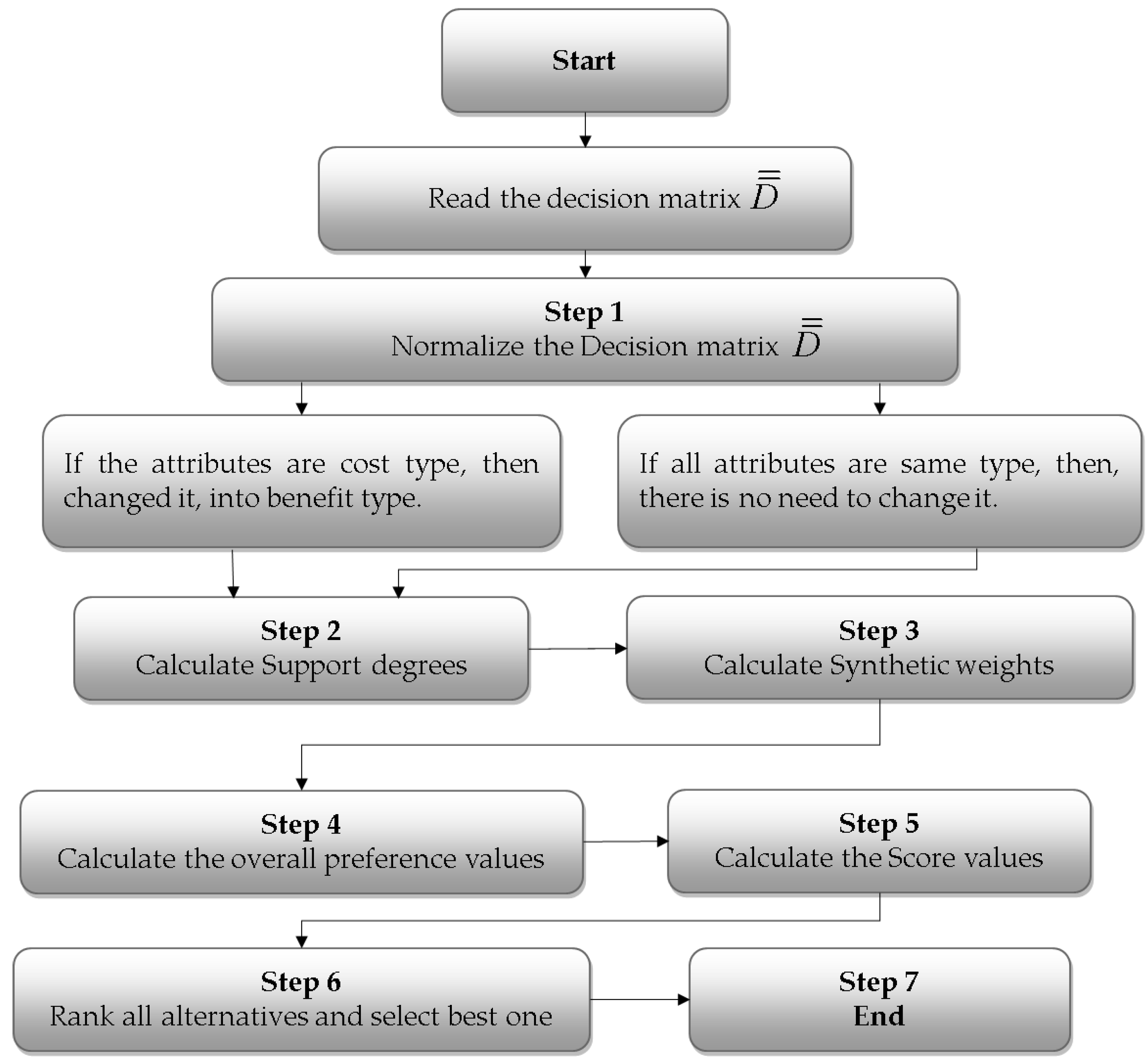
In this section, based upon the developed INWDPBM and INWDPGBM operators, we will propose a novel MADM method, which is defined as follows.

Assume that in a MADM problem, we need to evaluate $u$ alternatives $\tilde{M}=\left\{{\tilde{M}}_1,{\tilde{M}}_2,\dots ,{\tilde{M}}_u\right\}$ with respect to $v$ attributes $\tilde{C}=\left\{{\tilde{C}}_1,{\tilde{C}}_2,\dots ,{\tilde{C}}_v\right\}$, and the importance degree of the attributes is represented by $\varpi ={\left({\varpi }_1,{\varpi }_2,\dots ,{\varpi }_v\right)}^T$, satisfying the condition ${\varpi }_h\in \left[0,1\right],{\displaystyle \sum _{h=1}^v{\varpi }_h=1}$. The decision matrix for this decision problem is denoted by $\tilde{D}={\left[{\tilde{d}}_{gh}\right]}_{m\times n}$, where ${\tilde{d}}_{gh}=\langle \left[{\overline{\overline{TR}}}_{gh}^L,{\overline{\overline{TR}}}_{gh}^U\right],\left[{\overline{\overline{ID}}}_{gh}^L,{\overline{\overline{ID}}}_{gh}^U\right],\left[{\overline{\overline{FL}}}_{gh}^L{\overline{\overline{FL}}}_{gh}^U\right]\rangle$ is an INN for the alternative ${\tilde{M}}_g$ with respect to the attribute ${\tilde{C}}_h$, $\left(g=1,2,\dots ,u;h=1,2,\dots ,v\right).$ Then the main purpose is to rank the alternative and select the best alternative.

In the following, we will use the proposed INWDPBM and INWDPGBM operators to solve this MADM problem, and the detailed decision steps are shown as follows:

Step 1.

Standardize the attribute values. Normally, in real problems, the attributes are of two types, (1) cost type, (2) benefit type. To get right result, it is necessary to change cost type of attribute values to benefit type using the following formula:

$${\tilde{d}}_{gh}=\langle \left[{\overline{\overline{FL}}}_{gh}^L,{\overline{\overline{FL}}}_{gh}^U\right],\left[1-{\overline{\overline{ID}}}_{gh}^U,1-{\overline{\overline{ID}}}_{gh}^L\right],\left[{\overline{\overline{TR}}}_{gh}^L,{\overline{\overline{TR}}}_{gh}^U\right]\rangle .$$

(47)

Step 2.

Calculate the supports

$$Supp\left({\tilde{d}}_{gh},{\tilde{d}}_{gl}\right)=1-D\left({\tilde{d}}_{gh},{\tilde{d}}_{gl}\right),(g=1,2,\dots ,u;h,l=1,2,\dots ,v),$$

(48)

where, $D\left({\tilde{d}}_{gh},{\tilde{d}}_{gl}\right)$ is the distance measure defined in Equation (10).

Step 3.

Calculate $T\left({\tilde{d}}_{gh}\right)$

$$T\left({\tilde{d}}_{gh}\right)={\displaystyle \sum _{\begin{array}{l}l=1\\ l\ne h\end{array}}^{u}Supp\left({\tilde{d}}_{gh},{\tilde{d}}_{gl}\right),\left(g=1,2,\dots ,u;h,l=1,2,\dots ,v\right)}.$$

(49)

Step 4.

Aggregate all the attribute values ${\tilde{d}}_{gh}(h=1,2,\dots ,v)$ to the comprehensive value $R_g$ by using INWDPBM or INWDPGBM operators shown as follows.

$$R_g=INWDPBM\left({\tilde{d}}_{g1},{\tilde{d}}_{g2},\dots ,{\tilde{d}}_{gv}\right);$$

(50)

or

$$R_g=INWDPGBM\left({\tilde{d}}_{g1},{\tilde{d}}_{g2},\dots ,{\tilde{d}}_{gv}\right).$$

(51)

Step 5.

Determine the score values, accuracy values of $R_g(g=1,2,\dots ,u),$ using Definition 5.

Step 6.

Rank all the alternatives according to their score and accuracy values, and select the best alternative using Definition 6.

Step 7.

End.

This decision steps are also described in Figure 1.

6. Illustrative Example

In this part, an example adapted from [42] is used to illustrate the application and effectiveness of the developed method in MADM problem.

An investment company wants to invest a sum of money in the best option. The company must invest a sum of money in the following four possible companies (alternatives): (1) car company ${\tilde{M}}_1$; (2) food company ${\tilde{M}}_2$; (3) Computer company ${\tilde{M}}_3$; (4) An arm company ${\tilde{M}}_4$, and the attributes under consideration are (1) risk analysis ${\tilde{C}}_1$; (2) growth analysis ${\tilde{C}}_2$; (3) environmental impact analysis ${\tilde{C}}_3$. The importance degree of the attributes is $\varpi ={\left(0.35,0.4,0.25\right)}^T$. The four possible alternatives ${\tilde{M}}_g(g=1,2,3,4)$ are evaluated with respect to the above attributes ${\tilde{C}}_h\left(h=1,2,3\right)$ by the form of INN, and the IN decision matrix $\tilde{D}$ is listed in

Table 1. The IN decision matrix $\overline{\overline{D}}$.

Alternatives/Attributes	${\tilde{\mathit{C}}}_{\mathbf{1}}$	${\tilde{\mathit{C}}}_{\mathbf{2}}$	${\tilde{\mathit{C}}}_{\mathbf{3}}$
${\tilde{M}}_1$	$\langle \left[0.4,0.5\right],\left[0.2,0.3\right],\left[0.3,0.4\right]\rangle$	$\langle \left[0.4,0.6\right],\left[0.1,0.3\right],\left[0.2,0.4\right]\rangle$	$\langle \left[0.7,0.9\right],\left[0.7,0.8\right],\left[0.4,0.5\right]\rangle$
${\tilde{M}}_2$	$\langle \left[0.6,0.8\right],\left[0.1,0.2\right],\left[0.1,0.2\right]\rangle$	$\langle \left[0.6,0.7\right],\left[0.15,0.25\right],\left[0.2,0.3\right]\rangle$	$\langle \left[0.3,0.6\right],\left[0.2,0.3\right],\left[0.8,0.9\right]\rangle$
${\tilde{M}}_3$	$\langle \left[0.3,0.6\right],\left[0.2,0.3\right],\left[0.3,0.4\right]\rangle$	$\langle \left[0.5,0.6\right],\left[0.2,0.3\right],\left[0.3,0.4\right]\rangle$	$\langle \left[0.4,0.5\right],\left[0.2,0.4\right],\left[0.7,0.9\right]\rangle$
${\tilde{M}}_4$	$\langle \left[0.7,0.8\right],\left[0.01,0.1\right],\left[0.2,0.3\right]\rangle$	$\langle \left[0.6,0.7\right],\left[0.1,0.2\right],\left[0.3,0.4\right]\rangle$	$\langle \left[0.4,0.6\right],\left[0.5,0.6\right],\left[0.8,0.9\right]\rangle$

. The purpose of this decision-making problem is to rank the alternatives.

.

6.1. The Decision-Making Steps

Step 1.

Since ${\tilde{C}}_1,{\tilde{C}}_2$ are of benefit type, and ${\tilde{C}}_3$ is of cost type. So, ${\tilde{C}}_3$ will be changed into benefit type using Equation (47). So, the normalize decision matrix $\overline{\overline{D}}$ is given in

Table 2. The Normalize IN decision matrix $\overline{\overline{D}}$.

Alternatives/Attributes	${\tilde{\mathit{C}}}_{\mathbf{1}}$	${\tilde{\mathit{C}}}_{\mathbf{2}}$	${\tilde{\mathit{C}}}_{\mathbf{3}}$
${\tilde{M}}_1$	$\langle \left[0.4,0.5\right],\left[0.2,0.3\right],\left[0.3,0.4\right]\rangle$	$\langle \left[0.4,0.6\right],\left[0.1,0.3\right],\left[0.2,0.4\right]\rangle$	$\langle \left[0.4,0.5\right],\left[0.2,0.3\right],\left[0.7,0.9\right]\rangle$
${\tilde{M}}_2$	$\langle \left[0.6,0.8\right],\left[0.1,0.2\right],\left[0.1,0.2\right]\rangle$	$\langle \left[0.6,0.7\right],\left[0.15,0.25\right],\left[0.2,0.3\right]\rangle$	$\langle \left[0.8,0.9\right],\left[0.6,0.7\right],\left[0.3,0.6\right]\rangle$
${\tilde{M}}_3$	$\langle \left[0.3,0.6\right],\left[0.2,0.3\right],\left[0.3,0.4\right]\rangle$	$\langle \left[0.5,0.6\right],\left[0.2,0.3\right],\left[0.3,0.4\right]\rangle$	$\langle \left[0.7,0.9\right],\left[0.6,0.8\right],\left[0.4,0.5\right]\rangle$
${\tilde{M}}_4$	$\langle \left[0.7,0.8\right],\left[0.01,0.1\right],\left[0.2,0.3\right]\rangle$	$\langle \left[0.6,0.7\right],\left[0.1,0.2\right],\left[0.3,0.4\right]\rangle$	$\langle \left[0.8,0.9\right],\left[0.4,0.5\right],\left[0.4,0.6\right]\rangle$

.

Step 2.

Determine the supports $Supp\left({\tilde{d}}_{gh},{\tilde{d}}_{gl}\right),(g=1,2,3,4;h,l=1,2,3)$ by Equation (48) (for simplicity we denote $Supp\left({\tilde{d}}_{gh},{\tilde{d}}_{gl}\right)$ with $S_{gh,gl}^g$), we have

$$\begin{array}{l}{S}_{11,12}^1=S_{12,11}^1=0.950;S_{12,13}^1=S_{13,12}^1=0.800;S_{11,13}^1=S_{13,11}^1=0.85;S_{11,12}^2=S_{12,11}^2=0.933;S_{12,13}^2=S_{13,12}^2=0.717;S_{11,13}^2=S_{13,11}^2=0.683;\\ S_{11,12}^3=S_{12,11}^3=0.967;S_{12,13}^3=S_{13,12}^3=0.733;S_{11,13}^3=S_{13,11}^3=0.700;S_{11,12}^4=S_{12,11}^4=0.902;S_{12,13}^4=S_{13,12}^4=0.783;S_{11,13}^4=S_{13,11}^4=0.752;\end{array}$$

Step 3.

Determine $T\left({\tilde{d}}_{gh}\right);(g=1,2,3,4;h=1,2,3)$ by Equation (49), and we get

$$\begin{array}{l}{T}_{11}^1=1.800,T_{12}^1=1.750,T_{13}^1=1.650,T_{11}^2=1.617,T_{12}^2=1.650,T_{13}^2=1.400,\\ T_{11}^3=1.667,T_{12}^3=1.700,T_{13}^3=1.433,T_{11}^4=1.653,T_{12}^4=1.685,T_{13}^4=1.535.\end{array}$$

Step 4.

(a) 

Determine the comprehensive value of every alternative using the INWDPBM operator, that is, Equation (50) $\left(Assumethatx=y=1;\gamma =3\right)$, we have

$$R_1=\langle \left[0.3974,0.5195\right],\left[0.1823,0.3023\right],\left[0.3353,0.4796\right]\rangle ;$$

$$R_2=\langle \left[0.6457,0.7954\right],\left[0.1700,0.2885\right],\left[0.2044,0.3265\right]\rangle ;$$

$$R_3=\langle \left[0.4846,0.6503\right],\left[0.2556,0.3711\right],\left[0.3376,0.4394\right]\rangle ;$$

$$R_4=\langle \left[0.6938,0.7953\right],\left[0.1062,0.2154\right],\left[0.3069,0.4278\right]\rangle .$$

(b) 

Determine the comprehensive value of every alternative using the INWDPGBM operator, that is Equation (51), $\left(Assumethatx=y=1;\gamma =3\right)$, we have

$$R_1=\langle \left[0.4026,0.5381\right],\left[0.1570,0.2977\right],\left[0.2998,0.4520\right]\rangle ;$$

$$R_2=\langle \left[0.6654,0.8193\right],\left[0.1558,0.2686\right],\left[0.1836,0.3035\right]\rangle ;$$

$$R_3=\langle \left[0.5159,0.6732\right],\left[0.2366,0.3473\right],\left[0.3265,0.4279\right]\rangle ;$$

$$R_4=\langle \left[0.5159,0.8193\right],\left[0.0938,0.1952\right],\left[0.2862,0.4037\right]\rangle .$$

Step 5.

(a) 

Determine the score values of $R_g(g=1,2,3,4)$ by Definition 5, we have

$$S(R_1)=1.8087,S(R_2)=2.2259,S(R_3)=1.8656,S(R_4)=2.2164;$$

(b) 

Determine the score values of $R_g(g=1,2,3,4)$ by Definition 5, we have

$$S(R_1)=1.8671,S(R_2)=2.2866,S(R_3)=1.9254,S(R_4)=2.1781;$$

Step 6.

(a) 

According to their score and accuracy values, by using Definition 6, the ranking order is ${\tilde{M}}_2>{\tilde{M}}_4>{\tilde{M}}_3>{\tilde{M}}_1.$ So the best alternative is ${\tilde{M}}_2,$ while the worst alternative is ${\tilde{M}}_1.$

(b) 

According to their score and accuracy values, by using Definition 6, the ranking order is ${\tilde{M}}_2>{\tilde{M}}_4>{\tilde{M}}_3>{\tilde{M}}_1.$ So the best alternative is ${\tilde{M}}_2,$ while the worst alternative is ${\tilde{M}}_1.$

So, by using INWDPBM or INWDPGBM operators, the best alternative is ${\tilde{M}}_2,$ while the worst alternative is ${\tilde{M}}_1.$

6.2. Effect of Parameters $\gamma$, $x$ and $y$ on Ranking Result of this Example

In order to show the effect of the parameters x and $y$ on the ranking result of this example, we set different parameter values for $x$ and $y$, and $\gamma =3$ is fixed, to show the ranking results of this example. The ranking results are given in

Table 3. Ranking orders of decision result using different values for $x$ and $y$ for INWDPBM.

Parameter Values	INWDPBM Operator	Ranking Orders
$x=1,y=0,\gamma =3$	$\begin{array}{l}S(R_1)=1.9319,S(R_2)=2.4172,\\ S(R_3)=2.0936,S(R_4)=2.4222;\end{array}$	${\tilde{M}}_4>{\tilde{M}}_2>{\tilde{M}}_3>{\tilde{M}}_1.$
$x=1,y=5,\gamma =3$	$\begin{array}{l}S(R_1)=1.8338,S(R_2)=2.2684,\\ S(R_3)=1.9049,S(R_4)=2.2666;\end{array}$	${\tilde{M}}_2>{\tilde{M}}_4>{\tilde{M}}_3>{\tilde{M}}_1.$
$x=3,y=7,\gamma =3$	$\begin{array}{l}S(R_1)=1.8169,S(R_2)=2.2398,\\ S(R_3)=1.8777,S(R_4)=2.2327;\end{array}$	${\tilde{M}}_2>{\tilde{M}}_4>{\tilde{M}}_3>{\tilde{M}}_1.$
$x=5,y=10,\gamma =3$	$\begin{array}{l}S(R_1)=1.8143,S(R_2)=2.2354,\\ S(R_3)=1.8738,S(R_4)=2.2275;\end{array}$	${\tilde{M}}_4>{\tilde{M}}_2>{\tilde{M}}_3>{\tilde{M}}_1.$
$x=1,y=10,\gamma =3$	$\begin{array}{l}S(R_1)=1.8501,S(R_2)=2.2966,\\ S(R_3)=1.9355,S(R_4)=2.3012;\end{array}$	${\tilde{M}}_4>{\tilde{M}}_2>{\tilde{M}}_3>{\tilde{M}}_1.$
$x=10,y=4,\gamma =3$	$\begin{array}{l}S(R_1)=1.8182,S(R_2)=2.2419,\\ S(R_3)=1.8796,S(R_4)=2.2352;\end{array}$	${\tilde{M}}_4>{\tilde{M}}_2>{\tilde{M}}_3>{\tilde{M}}_1.$
$x=3,y=12,\gamma =3$	$\begin{array}{l}S(R_1)=1.8285,S(R_2)=2.2592,\\ S(R_3)=1.8958,S(R_4)=2.2557;\end{array}$	${\tilde{M}}_2>{\tilde{M}}_4>{\tilde{M}}_3>{\tilde{M}}_1.$

.

As we know from Table 3 and

Table 4. Ranking orders of decision result using different values for $x$ and $y$ for INWDPGBM.

Parameter Values	INWDPGBM Operator	Ranking Orders
$x=1,y=0,\gamma =3$	$\begin{array}{l}S(R_1)=1.5032,S(R_2)=1.7934,\\ S(R_3)=1.5136,S(R_4)=1.8037;\end{array}$	${\tilde{M}}_4>{\tilde{M}}_2>{\tilde{M}}_3>{\tilde{M}}_1.$
$x=1,y=5,\gamma =3$	$\begin{array}{l}S(R_1)=1.8220,S(R_2)=2.2256,\\ S(R_3)=1.8717,S(R_4)=2.1140;\end{array}$	${\tilde{M}}_2>{\tilde{M}}_4>{\tilde{M}}_3>{\tilde{M}}_1.$
$x=3,y=7,\gamma =3$	$\begin{array}{l}S(R_1)=1.8539,S(R_2)=2.2686,\\ S(R_3)=1.9094,S(R_4)=2.1584;\end{array}$	${\tilde{M}}_2>{\tilde{M}}_4>{\tilde{M}}_3>{\tilde{M}}_1.$
$x=5,y=10,\gamma =3$	$\begin{array}{l}S(R_1)=1.8583,S(R_2)=2.2745,\\ S(R_3)=1.9146,S(R_4)=2.1647;\end{array}$	${\tilde{M}}_2>{\tilde{M}}_4>{\tilde{M}}_3>{\tilde{M}}_1.$
$x=1,y=10,\gamma =3$	$\begin{array}{l}S(R_1)=1.7814,S(R_2)=2.1710,\\ S(R_3)=1.8248,S(R_4)=2.0632;\end{array}$	${\tilde{M}}_2>{\tilde{M}}_4>{\tilde{M}}_3>{\tilde{M}}_1.$
$x=10,y=4,\gamma =3$	$\begin{array}{l}S(R_1)=1.8087,S(R_2)=2.2259,\\ S(R_3)=1.8656,S(R_4)=2.2164;\end{array}$	${\tilde{M}}_2>{\tilde{M}}_4>{\tilde{M}}_3>{\tilde{M}}_1.$
$x=3,y=12,\gamma =3$	$\begin{array}{l}S(R_1)=1.8671,S(R_2)=2.2866,\\ S(R_3)=1.9254,S(R_4)=2.1781;\end{array}$	${\tilde{M}}_4>{\tilde{M}}_2>{\tilde{M}}_3>{\tilde{M}}_1.$

, the score values and ranking order are different for different values of the parameters $x$ and $y$, when we use INWDPBM operator and INWDPGBM operator. We can see from Table 3 and Table 4, when the parameter values x = 1 or 0 and y = 0 or 1, the best choice is ${\tilde{M}}_4$ and the worst one is ${\tilde{M}}_1.$ In simple words, when the interrelationship among attributes are not considered, the best choice is ${\tilde{M}}_4$ and the worst one is ${\tilde{M}}_1.$ On the other hand, when different values for the parameters $x$ and $y$ are utilized, for INWPBM and INWDPGBM operators, the ranking result is changed. That is, from Table 4, we can see that when the parameter values $x=1,y=1$, the ranking results are changed as the one obtained for x = 1 or 0 and y = 0 or 1. In this case the best alternative is ${\tilde{M}}_2$ while the worst alternative remains the same.

From Table 3 and Table 4, we can observe that when the values of the parameter increase, the score values obtained using INWDPBM decrease. While using the INWDPGBM operator, the score values increase but the best choice is $M_2$ for $x=y\ge 1$.

From

Table 5. Ranking orders of decision result using different values for $\gamma$.

Parameter Values	INWDPBM Operator	INWDPGBM Operator	Ranking Orders
$x=1,y=1,\gamma =0.5$	$\begin{array}{l}S(R_1)=1.6662,S(R_2)=2.1025,\\ S(R_3)=1.7606,S(R_4)=2.1972;\end{array}$	$\begin{array}{l}S(R_1)=1.7870,S(R_2)=2.2347,\\ S(R_3)=1.9103,S(R_4)=2.1812;\end{array}$	${\tilde{M}}_4>{\tilde{M}}_2>{\tilde{M}}_3>{\tilde{M}}_1.$ ${\tilde{M}}_2>{\tilde{M}}_4>{\tilde{M}}_3>{\tilde{M}}_1.$
$x=1,y=1,\gamma =2$	$\begin{array}{l}S(R_1)=1.7783,S(R_2)=2.2015,\\ S(R_3)=1.8408,S(R_4)=2.2091;\end{array}$	$\begin{array}{l}S(R_1)=1.8491,S(R_2)=2.2786,\\ S(R_3)=1.9213,S(R_4)=2.1799;\end{array}$	${\tilde{M}}_4>{\tilde{M}}_2>{\tilde{M}}_3>{\tilde{M}}_1.$ ${\tilde{M}}_2>{\tilde{M}}_4>{\tilde{M}}_3>{\tilde{M}}_1.$
$x=1,y=1,\gamma =4$	$\begin{array}{l}S(R_1)=1.8229,S(R_2)=2.2363,\\ S(R_3)=1.8803,S(R_4)=2.2219;\end{array}$	$\begin{array}{l}S(R_1)=1.8740,S(R_2)=2.2856,\\ S(R_3)=1.9275,S(R_4)=2.1751;\end{array}$	${\tilde{M}}_2>{\tilde{M}}_4>{\tilde{M}}_3>{\tilde{M}}_1.$ ${\tilde{M}}_2>{\tilde{M}}_4>{\tilde{M}}_3>{\tilde{M}}_1.$
$x=1,y=1,\gamma =7$	$\begin{array}{l}S(R_1)=1.8375,S(R_2)=2.2455,\\ S(R_3)=1.9037,S(R_4)=2.2315;\end{array}$	$\begin{array}{l}S(R_1)=1.8747,S(R_2)=2.2763,\\ S(R_3)=1.9331,S(R_4)=2.1669;\end{array}$	${\tilde{M}}_2>{\tilde{M}}_4>{\tilde{M}}_3>{\tilde{M}}_1.$ ${\tilde{M}}_2>{\tilde{M}}_4>{\tilde{M}}_3>{\tilde{M}}_1.$
$x=1,y=1,\gamma =10$	$\begin{array}{l}S(R_1)=1.8418,S(R_2)=2.2477,\\ S(R_3)=1.9160,S(R_4)=2.2365;\end{array}$	$\begin{array}{l}S(R_1)=1.8701,S(R_2)=2.2698,\\ S(R_3)=1.9373,S(R_4)=2.1622;\end{array}$	${\tilde{M}}_2>{\tilde{M}}_4>{\tilde{M}}_3>{\tilde{M}}_1.$ ${\tilde{M}}_2>{\tilde{M}}_4>{\tilde{M}}_3>{\tilde{M}}_1.$
$x=1,y=1,\gamma =15$	$\begin{array}{l}S(R_1)=1.8447,S(R_2)=2.2488,\\ S(R_3)=1.9270,S(R_4)=2.2409;\end{array}$	$\begin{array}{l}S(R_1)=1.8642,S(R_2)=2.2637,\\ S(R_3)=1.9414,S(R_4)=2.1582;\end{array}$	${\tilde{M}}_2>{\tilde{M}}_4>{\tilde{M}}_3>{\tilde{M}}_1.$ ${\tilde{M}}_2>{\tilde{M}}_4>{\tilde{M}}_3>{\tilde{M}}_1.$
$x=1,y=1,\gamma =20$	$\begin{array}{l}S(R_1)=1.8460,S(R_2)=2.2492,\\ S(R_3)=1.9328,S(R_4)=2.2432;\end{array}$	$\begin{array}{l}S(R_1)=1.8608,S(R_2)=2.2604,\\ S(R_3)=1.9435,S(R_4)=2.1562;\end{array}$	${\tilde{M}}_2>{\tilde{M}}_4>{\tilde{M}}_3>{\tilde{M}}_1.$ ${\tilde{M}}_2>{\tilde{M}}_4>{\tilde{M}}_3>{\tilde{M}}_1.$

, we can see that different ranking orders are obtained for different values of $\gamma$. When $\gamma =0.5\mathrm{and}\gamma =2$, the best choice is $M_4$ by the INWPBM operator; when we use the INWPGBM operator, it is $M_2$. Similarly, for other values of $\gamma >2$, the best choice is $M_2$ while the worst is $M_1$.

6.3. Comparing with the Other Methods

To illustrate the advantages and effectiveness of the developed method in this article, we solve the above example by four existing MADM methods, including IN weighted averaging operator, IN weighted geometric operator [12], the similarity measure defined by Ye [15], Muirhead mean operators developed by Liu et al. [42], IN power aggregation operator developed by Liu et al. [37].

From

Table 6. Ranking order of the alternatives using different aggregation operators.

Aggregation Operator	Parameter	Score Values	Ranking Order
INWA operator [12]	No	$\begin{array}{l}S(R_1)=1.8430,S(R_2)=2.2497,\\ S(R_3)=1.9151,S(R_4)=2.2788;\end{array}$	${\tilde{M}}_4>{\tilde{M}}_2>{\tilde{M}}_3>{\tilde{M}}_1.$
INWGA operator [12]	No	$\begin{array}{l}S(R_1)=1.7286,S(R_2)=2.0991,\\ S(R_3)=1.7751,S(R_4)=2.1608;\end{array}$	${\tilde{M}}_4>{\tilde{M}}_2>{\tilde{M}}_3>{\tilde{M}}_1.$
Similarity measure Hamming distance [15]	No	$\begin{array}{l}{D}_1(R^{\ast },R_1)=0.7948,D_1(R^{\ast },R_2)=0.9581,\\ D_1(R^{\ast },R_3)=0.8805,D_1(R^{\ast },R_4)=0.9725;\end{array}$	${\tilde{M}}_4>{\tilde{M}}_2>{\tilde{M}}_3>{\tilde{M}}_1.$
Generalized power Aggregation operator [37]	Yes $\lambda =1$	$\begin{array}{l}S(R_1)=1.8460,S(R_2)=2.2543,\\ S(R_3)=1.9163,\mathrm{S}(R_4)=2.2799;\end{array}$	${\tilde{M}}_4>{\tilde{M}}_2>{\tilde{M}}_3>{\tilde{M}}_1.$
INWMM operator [42]	Yes $P(1,1,1)$	$\begin{array}{l}S(R_1)=1.8054,S(R_2)=2.2321,\\ S(R_3)=1.9172,\mathrm{S}(R_4)=2.2773;\end{array}$	${\tilde{M}}_4>{\tilde{M}}_2>{\tilde{M}}_3>{\tilde{M}}_1.$
INWDMM operator [42]	Yes $P(1,1,1)$	$\begin{array}{l}S(R_1)=1.6260,S(R_2)=1.9202,\\ S(R_3)=1.7061,\mathrm{S}(R_4)=2.0798;\end{array}$	${\tilde{M}}_4>{\tilde{M}}_2>{\tilde{M}}_3>{\tilde{M}}_1.$
Proposed INWDPBM $x=1,y=0,\gamma =3$	Yes	$\begin{array}{l}S(R_1)=1.9319,S(R_2)=2.4172,\\ S(R_3)=2.0936,S(R_4)=2.4222;\end{array}$	${\tilde{M}}_4>{\tilde{M}}_2>{\tilde{M}}_3>{\tilde{M}}_1.$
Proposed INWDPGBM $x=1,y=0,\gamma =3$	Yes	$\begin{array}{l}S(R_1)=1.5032,S(R_2)=1.7934,\\ S(R_3)=1.5136,S(R_4)=1.8037;\end{array}$	${\tilde{M}}_4>{\tilde{M}}_2>{\tilde{M}}_3>{\tilde{M}}_1.$
INWDPBM operator in this article	Yes $x=y=1,\gamma =3$	$\begin{array}{l}S(R_1)=1.8087,S(R_2)=2.2259,\\ S(R_3)=1.8656,S(R_4)=2.2164;\end{array}$	${\tilde{M}}_2>{\tilde{M}}_4>{\tilde{M}}_3>{\tilde{M}}_1.$
INWDPBM operator in this article	Yes $x=y=1,\gamma =3$	$\begin{array}{l}S(R_1)=1.8671,S(R_2)=2.2866,\\ S(R_3)=1.9254,S(R_4)=2.1781;\end{array}$	${\tilde{M}}_2>{\tilde{M}}_4>{\tilde{M}}_3>{\tilde{M}}_1.$

, we can see that the ranking orders are the same as the ones produced by the existing aggregation operators when the parameter values $x=1,y=0,\gamma =3$, but the ranking orders are different when the interrelationship among attributes are considered. That is why the developed method based on the proposed aggregation operators is more flexible due the parameter and practical as it can consider the interrelationship among input arguments.

From the above comparative analysis, we can know the proposed method has the following advantages, that is, it can consider the interrelationship among the input arguments and can relieve the effect of the awkward data by PWV at the same time, and it can permit more precise ranking order than the existing methods. The proposed method can take the advantages of PA operator and BM operator concurrently, these factors makes it a little complex in calculations.

The score values and ranking orders by these methods are shown in Table 6.

7. Conclusions

The PBM operator can take the advantage of PA operator, which can eliminate the impact of awkward data given by the predisposed DMs, and BM operator, which can consider the correlation between two attributes. The Dombi operations of TN and TCN proposed by Dombi have the edge of good flexibility with general parameter. In this article, we combined PBM with Dombi operation and proposed some aggregation operators to aggregate INNs. Firstly, we defined some operational laws for INSs based on Dombi TN and TCN and discussed some properties of these operations. Secondly, we extended PBM operator based on Dombi operations to introduce INDPBM operator, INWDPBM operator, INDPGBM operator, INWDPGBM operator and discussed some properties of these aggregation operators. The developed aggregation operators have the edge that they can take the correlation among the attributes by BM operator, and can also remove the effect of awkward data by PA operator at the same and due to general parameter, so they are more flexible in the aggregation process. Further, we developed a novel MADM method based on developed aggregation operators to deal with interval neutrosophic information. Finally, an illustrative example is used to show the effectiveness and practicality of the proposed MADM method and comparison were made with the existing methods. The proposed aggregation operators are very useful to solve MADM problems.

In future research, we shall define some distinct aggregation operators for SVHFSs, INHFSs, double valued neutrosophic sets and so on based on Dombi operations and apply them to MAGDM and MADM.

References

1. Zadeh, L.A. Fuzzy sets. Inf. Control 1965, 8, 338–353. [Google Scholar] [CrossRef] [Green Version]
2. Medina, J.; Ojeda-Aciego, M. Multi-adjoint t-concept lattices. Inf. Sci. 2010, 180, 712–725. [Google Scholar] [CrossRef]
3. Pozna, C.; Minculete, N.; Precup, R.E.; Kóczy, L.T.; Ballagi, A. Signatures: Definitions, operators and applications to fuzzy modelling. Fuzzy Sets Syst. 2012, 201, 86–104. [Google Scholar] [CrossRef]
4. Kumar, A.; Kumar, D.; Jarial, S.K. A hybrid clustering method based on improved artificial bee colony and fuzzy C-Means algorithm. Int. J. Artif. Intell. 2017, 15, 24–44. [Google Scholar]
5. Turksen, I.B. Interval valued fuzzy sets based on normal forms. Fuzzy Sets Syst. 1986, 20, 191–210. [Google Scholar] [CrossRef]
6. Atanassov, K.T. Intuitionistic fuzzy sets. Fuzzy Sets Syst. 1986, 20, 87–96. [Google Scholar] [CrossRef]
7. Atanassov, K.; Gargov, G. Interval valued intuitionistic fuzzy sets. Fuzzy Sets Syst. 1989, 31, 343–349. [Google Scholar] [CrossRef]
8. Smarandache, F. Neutrosophic Probability, Set, and Logic. In Neutrosophy; American Research Press: Rehoboth, IL, USA, 1998. [Google Scholar]
9. Smarandache, F. Neutrosophic set—A generalization of the intuitionistic fuzzy set. Int. J. Pure Appl. Math. 2010, 1, 107–116. [Google Scholar]
10. Wang, H.; Smarandache, F.; Zhang, Y.; Sunderraman, R. Single valued neutrosophic sets. In Proceedings of the 8th joint conference on information Sciences, Salt Lake City, UT, USA, 21–26 July 2005; pp. 94–97. [Google Scholar]
11. Wang, H.; Smarandache, F.; Sunderraman, R.; Zhang, Y.Q. Interval Neutrosophic Sets and Logic: Theory and Application in Computing; Hexis: Phoenix, AZ, USA, 2005. [Google Scholar]
12. Zhang, H.Y.; Wang, J.Q.; Chen, X.H. Interval neutrosophic sets and their application in multi-criteria decision making problems. Sci. World J. 2014, 2014, 645953. [Google Scholar] [CrossRef]
13. Ye, J. A multi-criteria decision-making method using aggregation operators for simplified neutrosophic sets. J. Intell. Fuzzy Syst. 2014, 26, 2459–2466. [Google Scholar] [CrossRef]
14. Peng, J.J.; Wang, J.Q.; Wang, J.; Zhang, H.Y.; Chen, X.H. Simplified neutrosophic sets and their applications in multi-criteria group decision-making problems. Int. J. Syst. Sci. 2016, 47, 2342–2358. [Google Scholar] [CrossRef]
15. Ye, J. Similarity measures between interval neutrosophic sets and their applications in multicriteria decision-making. J. Intell. Fuzzy Syst. 2014, 26, 165–172. [Google Scholar] [CrossRef]
16. Broumi, S.; Smarandache, F. New distance and similarity measures of interval neutrosophic sets. In Proceedings of the 17th International Conference on Information Fusion (FUSION), Salamanca, Spain, 7–10 July 2014; pp. 1–7. [Google Scholar]
17. Broumi, S.; Smarandache, F. Cosine similarity measure of interval valued neutrosophic sets. Neutrosophic Sets Syst. 2014, 5, 15–20. [Google Scholar]
18. Ye, J.; Shigui, D. Some distances, similarity and entropy measures for interval-valued neutrosophic sets and their relationship. Int. J. Mach. Learn. Cybern. 2017, 1–9. [Google Scholar] [CrossRef]
19. Majumdar, P.; Samanta, S.K. On similarity and entropy of neutrosophic sets. J. Intell. Fuzzy Syst. 2014, 26, 1245–1252. [Google Scholar] [CrossRef]
20. Tian, Z.P.; Zhang, H.Y.; Wang, J.; Wang, J.Q.; Chen, X.H. Multi-criteria decision-making method based on a cross-entropy with interval neutrosophic sets. Int. J. Syst. Sci. 2016, 47, 3598–3608. [Google Scholar] [CrossRef]
21. Ye, J. Improved correlation coefficients of single valued neutrosophic sets and interval neutrosophic sets for multiple attribute decision making. J. Intell. Fuzzy Syst. 2014, 27, 2453–2462. [Google Scholar] [CrossRef]
22. Zhang, H.; Ji, P.; Wang, J.; Chen, X. An improved weighted correlation coefficient based on integrated weight for interval neutrosophic sets and its application in multi-criteria decision-making problems. Int. J. Comput. Intell. Syst. 2015, 8, 1027–1043. [Google Scholar] [CrossRef]
23. Ye, J. Multiple attribute decision-making method using correlation coefficients of normal neutrosophic sets. Symmetry 2017, 9, 80. [Google Scholar] [CrossRef]
24. Yu, D. Group decision making based on generalized intuitionistic fuzzy prioritized geometric operator. Int. J. Intell. Syst. 2012, 27, 635–661. [Google Scholar] [CrossRef]
25. Liu, P. Multiple attribute group decision making method based on interval-valued intuitionistic fuzzy power Heronian aggregation operators. Comput. Ind. Eng. 2017, 108, 199–212. [Google Scholar] [CrossRef]
26. Mahmood, T.; Liu, P.; Ye, J.; Khan, Q. Several hybrid aggregation operators for triangular intuitionistic fuzzy set and their application in multi-criteria decision making. Granul. Comput. 2018, 3, 153–168. [Google Scholar] [CrossRef]
27. Liao, H.; Xu, Z. Intuitionistic fuzzy hybrid weighted aggregation operators. Int. J. Intell. Syst. 2014, 29, 971–993. [Google Scholar] [CrossRef]
28. Xu, Z. Intuitionistic fuzzy aggregation operators. IEEE Trans. Fuzzy Syst. 2007, 15, 1179–1187. [Google Scholar] [CrossRef]
29. Xu, Z.; Yager, R.R. Some geometric aggregation operators based on intuitionistic fuzzy sets. Int. J. Gener. Syst. 2006, 35, 417–433. [Google Scholar] [CrossRef]
30. Sun, H.X.; Yang, H.X.; Wu, J.Z.; Ouyang, Y. Interval neutrosophic numbers Choquet integral operator for multi-criteria decision making. J. Intell. Fuzzy Syst. 2015, 28, 2443–2455. [Google Scholar] [CrossRef]
31. Liu, P.; Wang, Y. Interval neutrosophic prioritized OWA operator and its application to multiple attribute decision making. J. Syst. Sci. Complex. 2016, 29, 681–697. [Google Scholar] [CrossRef]
32. Mukhametzyanov, I.; Pamucar, D. A sensitivity analysis in MCDM problems A statistical approach. Decis. Mak. Appl. Manag. Eng. 2018, 1. [Google Scholar] [CrossRef]
33. Petrović, I.; Kankaraš, M. DEMATEL-AHP multi-criteria decision making model for the selection and evaluation of criteria for selecting an aircraft for the protection of air traffic. Decis. Mak. Appl. Manag. Eng. 2018, 1. [Google Scholar] [CrossRef]
34. Roy, J.; Adhikary, K.; Kar, S.; Pamučar, D. A rough strength relational DEMATEL model for analysing the key success factors of hospital service quality. Decis. Mak. Appl. Manag. Eng. 2018, 1, 121–142. [Google Scholar] [CrossRef]
35. Biswajit, S.; Sankar, P.M.; Sun, H.; Ali, A.; Soheil, S.; Rekha, G.; Muhammad, W.I. An optimization technique for national income determination model with stability analysis of differential equation in discrete and continuous process under the uncertain environment. RAIRO Oper. Res. 2018. [Google Scholar] [CrossRef]
36. Yager, R.R. The power average operator. IEEE Trans. Syst. Man Cybern. Part A 2001, 31, 724–731. [Google Scholar] [CrossRef]
37. Liu, P.; Tang, G. Some power generalized aggregation operators based on the interval neutrosophic sets and their application to decision making. J. Intell. Fuzzy Syst. 2016, 30, 2517–2528. [Google Scholar] [CrossRef]
38. Bonferroni, C. Sulle medie multiple di potenze. Bollettino dell’Unione Matematica Italiana 1950, 5, 267–270. [Google Scholar]
39. Sykora, S. Mathematical Means and Averages: Generalized Heronian Means. Stan’s Libr. 2009. [Google Scholar] [CrossRef]
40. Muirhead, R.F. Some methods applicable to identities and inequalities of symmetric algebraic functions of n letters. Proc. Edinb. Math. Soc. 1902, 21, 144–162. [Google Scholar] [CrossRef]
41. Maclaurin, C. A second letter to Martin Folkes, Esq.; concerning the roots of equations, with the demonstration of other rules of algebra. Philos. Trans. 1729, 36, 59–96. [Google Scholar]
42. Liu, P.; You, X. Interval neutrosophic Muirhead mean operators and their applications in multiple-attribute group decision making. Int. J. Uncertain. Quant. 2017, 7, 303–334. [Google Scholar] [CrossRef]
43. Qin, J.; Liu, X. An approach to intuitionistic fuzzy multiple attribute decision making based on Maclaurin symmetric mean operators. J. Intell. Fuzzy Syst. 2014, 27, 2177–2190. [Google Scholar] [CrossRef]
44. Li, Y.; Liu, P.; Chen, Y. Some single valued neutrosophic number Heronian mean operators and their application in multiple attribute group decision making. Informatica 2016, 27, 85–110. [Google Scholar] [CrossRef]
45. Xu, Z.; Yager, R.R. Intuitionistic fuzzy Bonferroni means. IEEE Trans. Syst. Man Cybern. Part B 2011, 41, 568–578. [Google Scholar] [CrossRef]
46. Zhou, W.; He, J.M. Intuitionistic fuzzy geometric Bonferroni means and their application in multi-criteria decision making. Int. J. Intell. Syst. 2012, 27, 995–1019. [Google Scholar] [CrossRef]
47. Dombi, J. A general class of fuzzy operators, the DeMorgan class of fuzzy operators and fuzziness measures induced by fuzzy operators. Fuzzy Sets Syst. 1982, 8, 149–163. [Google Scholar] [CrossRef]
48. Liu, P.; Liu, J.; Chen, S.H. Some intuitionistic fuzzy Dombi Bonferroni mean operators and their application to multi-attribute group decision making. J. Oper. Res. Soc. 2018, 69, 1–24. [Google Scholar] [CrossRef]
49. Chen, J.; Ye, J. Some single-valued neutrosophic Dombi weighted aggregation operators for multiple attribute decision-making. Symmetry 2017, 9, 82. [Google Scholar] [CrossRef]
50. Torra, V. Hesitant fuzzy sets. Int. J. Intell. Syst. 2010, 25, 529–539. [Google Scholar] [CrossRef]
51. He, X. Typhoon disaster assessment based on Dombi hesitant fuzzy information aggregation operators. Nat. Hazards 2018, 90, 1153–1175. [Google Scholar] [CrossRef]
52. He, Y.; He, Z.; Deng, Y.; Zhou, P. IFPBMs and their application to multiple attribute group decision making. J. Oper. Res. Soc. 2016, 67, 127–147. [Google Scholar] [CrossRef]
53. He, Y.; He, Z.; Jin, C.; Chen, H. Intuitionistic fuzzy power geometric Bonferroni means and their application to multiple attribute group decision making. Int. J. Uncertain. Fuzz. Knowl.-Based Syst. 2015, 23, 285–315. [Google Scholar] [CrossRef]
54. He, Y.; He, Z.; Wang, G.; Chen, H. Hesitant fuzzy power Bonferroni means and their application to multiple attribute decision making. IEEE Trans. Fuzzy Syst. 2015, 23, 1655–1668. [Google Scholar] [CrossRef]
55. Liu, P.; Liu, X. Multi-attribute group decision making methods based on linguistic intuitionistic fuzzy power Bonferroni mean operators. Complexity 2017, 2017, 1–15. [Google Scholar]
Figure 1. Flow chart for developed approach.
Symmetry 10 00459 g001