Deep Learning-Based Multinational Banknote Fitness Classification with a Combination of Visible-Light Reflection and Infrared-Light Transmission Images

Abstract

The fitness classification of a banknote is important as it assesses the quality of banknotes in automated banknote sorting facilities, such as counting or automated teller machines. The popular approaches are primarily based on image processing, with banknote images acquired by various sensors. However, most of these methods assume that the currency type, denomination, and exposed direction of the banknote are known. In other words, not only is a pre-classification of the type of input banknote required, but in some cases, the type of currency is required to be manually selected. To address this problem, we propose a multinational banknote fitness-classification method that simultaneously determines the fitness level of a banknote from multiple countries. This is achieved without the pre-classification of input direction and denomination of the banknote, using visible-light reflection and infrared-light transmission images of banknotes, and a convolutional neural network. The experimental results on the combined banknote image database consisting of the Indian rupee and Korean won with three fitness levels, and the United States dollar with two fitness levels, show that the proposed method achieves better accuracy than other fitness classification methods.

1. Introduction

Currently, automated machines for financial transactions are becoming popular and have been significantly modernized. Such facilities can handle various functionalities, including not only the recognition of banknote type, counting, sorting and detection of counterfeits, but also serial recognition and fitness classification [1]. The capability of operating on currencies from various countries and regions is also being considered. Among them, banknote fitness classification evaluates the physical condition of the banknotes that may be degraded during the recirculation process, and determines whether they are still usable or should be replaced by new ones. This also helps to enhance the performance of the counting and sorting functionalities, as well as preventing malfunctions and inconveniences caused by damaged banknotes entering the counting system.

The widely used approaches for the problems of automated banknote sorting are based on image processing techniques, in which the optical characteristics of banknotes are captured by various imaging sensors. Because the presentations of banknotes are different among different types of currencies, and between the front and reverse sides of the banknote, most of the studies on fitness classification assume that the currency type, denomination, and input direction of the presented banknote are known [1,2]. These studies were proposed for either a certain type of currency or multiple national currencies, and their fitness classification methods are explained in detail in the next section.

2. Related Works

Studies have been conducted that subject fitness classification to a certain national currency or to banknotes from various countries and regions. Considering soiling as the primary criterion for classifying the fitness levels of Euro banknotes (EUR) [3], Geusebroek et al. [4] and Balke et al. [5] proposed a method that evaluates soiling using the adaptive boosting (AdaBoost) algorithm with color images of the banknotes. The classification features are the mean and standard deviation values of the color channels’ intensity extracted from the overlapping rectangular regions on banknote images [4,5]. Another Euro banknote recognition system was proposed by Aoba et al. [6], based on the combination and processing of visible and infrared (IR) banknote images. In this system, the banknote types are classified by a three-layered perceptron, and banknote fitness is validated by radial basis function (RBF) networks [6]. For assessing the quality of Chinese banknotes (RMB), both the studies in [7,8] used the gray-level histogram of banknote images as the classification features, but employed different algorithms as the classifiers: neural network (NN) [7], and the combination of dynamic time warp (DTW) and support vector machine (SVM) [8]. Pham et al. [9] proposed a fitness classification method for the Indian rupee (INR) based on grayscale images captured by visible light sensors. In this study, they performed discrete wavelet transform (DWT) on preselected regions of interest (ROIs), calculated the mean and standard deviation features, and classified the fitness level of the banknotes using an SVM [9].

In the studies considering the variety of currencies, experiments were conducted with banknote datasets consisting of currency papers from various countries or regions. The fuzzy-based method using visible-light reflection (VR) and near-infrared light transmission (NIRT) images of the banknotes (proposed by Kwon et al. [10]) was tested with banknotes in the United States currency (USD), Indian currency (INR), and Korean currency (KRW). In [11], Lee et al. proposed a soiled banknote fitness determination based on morphology and Otsu’s thresholding on EUR and Russian ruble (RUB) banknote images, captured by a contact image sensor (CIS). The convolutional neural network (CNN)-based method proposed by Pham et al. [2] could classify the fitness levels regardless of the denomination, and the input direction of banknotes in each of the currencies of INR, KRW and USD.

The ability to simultaneously classify multiple currencies from various countries has been attracting research interest, primarily for the functionality of banknote type (national currency, denomination, and input direction) recognition. Studies have been conducted regarding the classification of banknotes from up to two different national currencies using various methods, such as NNs [12], NNs and genetic algorithms (GA) [13], correlation matching [14], linear discriminant analysis (LDA) [15], and the hidden Markov model (HMM) [16]. The recent CNN-based method proposed by Pham et al. [17] could simultaneously recognize banknotes from six countries with an accuracy of 100% and showed that the CNN could be a promising approach for the problem of multinational banknote classification. However, studies on banknote classification that utilize the advantages of CNNs are still limited. There have been studies in the field of computer vision classification that employed both handcrafted and non-handcrafted features. In the study of Nanni et al. [18], besides the network-based features, they considered various other handcrafted features such as local ternary patterns (LTP), local phase quantization (LPQ), local binary pattern (LBP), etc., and combined them in the classification task by score level fusion. The experimental results show that handcrafted and non-handcrafted features were able to extract different information from input images and their combination can help to boost the performance [18]. However, this method used multiple CNN models and methods for handcrafted image feature extraction and could make the classification system very complex. The CNN-based method proposed in [17] focused on classification of currency type, denomination and input direction of banknotes from multiple countries and did not consider the fitness for recirculation of banknotes. In the method using CNN in [2], the fitness classification tasks were conducted on separate currency types. Consequently, the types of currencies still need to be manually selected before their fitness for recirculation is evaluated. However, this research shows the fitness classification of multiple national currencies without any prior knowledge of currency type. In addition, both of these previous works [2,17] used only the grayscale VR banknotes image, which might show limited performance when dealing with the problem of simultaneously classifying of banknote fitness from multiple national currencies. As a result, banknote images acquired by multiple sensors for VR and infrared transmission (IRT) images are considered in this study for evaluation of fitness. Experimental results show that our method, using both VR and IRT images, outperforms those using only VR images.

Table 1. Comparison of the proposed method and previous works on the fitness classification of banknotes. EUR = Euro. RBF = radial basis function. IR = infrared. NN = neural network. DTW = dynamic time warp. SVM = support vector machine. VR = visible-light reflection. INR = Indian currency. CNN = convolutional neural network.

Category	Method	Advantage	Disadvantage
Fitness classification on single national currency	- Using features from color channels of EUR banknote images [4,5] - Using RBF for fitness validation in the EUR banknote recognition system with visible and IR images of banknotes [6]. - Using gray level histogram of Chinese banknote images for classification by using NN [7] or DTW and SVM [8]. - Using DWT for feature extraction on VR images of INR banknotes and classifying fitness by SVM [9].	Simplified feature selection as the fitness classification is conducted on the known (pre-classified) type of banknote.	Effectiveness of the fitness classification method is not confirmed on the other types of currencies.
Fitness classification on various national currencies	- Using the grayscale histogram of banknote images and classifying fitness using DTW and SVM [6] or using a NN [7]. - Using multiresolutional features of visible and IR images of banknote for recognition [8]. - Soiling evaluation based on image morphological operations and Otsu’s thresholding on banknote images [11].	The fitness classification method is tested on various types of currencies.	The types of currencies are still manually selected or pre-classified before determining the fitness
	Multinational banknote fitness classification using CNN (proposed method)	Fitness classification is simultaneously conducted on multiple countries’ banknotes.	Intensive training of the CNN is required.

summarizes the comparison between our method and a previous study. In Section 4, we explain the proposed multinational banknote fitness classification method in detail. The experimental results and conclusions are presented in Section 5 and Section 6, respectively.

3. Contributions

To address the problems in the previously proposed methods, we considered a multinational banknote fitness classification method using CNN on VR and IRT banknote images. In our proposed method, banknote images captured by various sensors are arranged into multiple channels to be the input to the CNN classifier. Through an intensive training process, our proposed system is designed to simultaneously classify the fitness of banknotes from multiple countries, regardless of the input banknote’s denomination and input direction. Compared to previous studies, the novelty of our method can be shown as follows:

-

This is the first study on multinational banknote fitness classification performed on INR, KRW, and USD currencies. Although the previous study could determine the banknote fitness levels without the pre-classification of banknote images in the denomination and input direction [2], the fitness classification tasks were still conducted on the separate currency types.

-

The images of the input banknote are captured by VR sensors on both sides in the cases of INR and KRW, and on the front side in the case of USD. In addition, IRT images are captured from the front side in all cases of INR, KRW, and USD. The captured images are arranged into a three-channel image to be input to the CNN classifier, with the VR channel duplicated in the case of USD. We included the USD banknote image dataset with a different number of sensors for capturing images from that of the remaining datasets of INR and KRW. Therefore, we can evaluate the robustness of the proposed method with various numbers of imaging sensors. Experimental results showed good performance regardless of the types of currency and the number of sensors for capturing banknote images.

-

With the three levels of fitness (namely fit, normal, and unfit) in the cases of INR and KRW (Case 1), and two levels of fit and unfit for USD (Case 2), the CNN classifier in our proposed method consists of five outputs to ensure the coverage of all the fitness classes in both cases.

-

We created the self-collected banknote fitness database of the Dongguk fitness database (DF-DB2), and trained the CNN model that is publicly available through the method in [19] such that other researchers can compare and evaluate the performance.

4. Proposed Method

4.1. Overview of the Proposed Method

Figure 1 shows the overall flowchart of the proposed method. The input banknote is captured by VR and NIRT. The captured images are subsequently passed to the preprocessing steps, in which the banknote regions are segmented from the background and resized to a consistent size of 115 × 51 pixels. The equally resized images of the input banknote are arranged into a three-channel image, in which the first channel is the IRT image, and the remainder is the VR images of both sides of the banknote. This combined image is input into the pretrained CNN to be classified for the fitness level at the network output.

4.2. Banknote Image Acquisition and Preprocessing

The banknote images are captured in the commercial counting machine that is equipped with imaging sensors capable of acquiring images in various wavelengths [20]. The analysis of the lighting mechanisms on new and old banknotes [10] shows that light reflection tends to be reduced by scattering on a rough surface, and light transmission is expected to be reduced owing to energy absorption by soiling materials. Consequently, we used VR and IRT images for the fitness classification in this study.

In the banknote-counting machine, line-contact image sensors are used rather than area sensors, for size and cost efficiency. For capturing the entire banknote, each image line comprising 1584 pixels is captured sequentially, one line for each triggering time. For the VR images, the trigger number when the input banknote is INR or KRW is 464, while that for USD banknotes is 350. For the IRT images, 116 line images are captured for INR or KRW, and 175 line images are captured for USD. These line images are concatenated for acquiring the final two-dimensional banknote images, in which the VR images and IRT images have resolutions of 1584 × 464 and 1584 × 116 pixels, respectively, for INR and KRW banknotes, and 1584 × 350 and 1584 × 175 pixels, respectively, for the USD banknotes.

The input banknote is inserted into the counting machine in one of the four directions, which are forward and backward directions of the front side, and forward and backward directions of the reverse side, labeled as A, B, C and D directions, respectively. After obtaining the banknote’s image, we used the built-in corner detection algorithm of the counting machine [2] to segment the banknote region from the background of the image. This task not only excludes the redundant information of the surrounding background, but also adjusts the displacement of the input banknote captured in the original image [17]. Examples of the captured banknote images by the machine with VR and IRT sensors for the INR banknote are shown in Figure 2.

The segmented banknote images are subsequently equally resized to 115 × 51 pixels, and arranged into a three-channel image for each input banknote, in which the first channel is the IRT image, and the second and third channels are the VR images of the front and reverse sides, respectively. This combined image is input to the CNN classifier in the next step.

4.3. The CNN Architecture

The CNN structure used in our proposed method consists of five convolutional layers, denoted as L1 to L5, and three fully connected layers, denoted as F1 to F3, as shown in Figure 3. This architecture is inspired by the AlexNet architecture [2,17,21]. The details of each layer’s attributes and the size of the feature map at each layer are shown in

Table 2. Details of the CNN and size of feature maps at each CNN’s layer (unit: pixel).

Layer Type		Kernel Attribute	Number of Filters	Feature Map Size
Image Input Layer				115 × 51 × 3
L1	Convolutional Layer	7 × 7 × 3, stride 2, no padding	96	55 × 23 × 96
	ReLU Layer
	CCN Layer
	Max Pooling	3 × 3, stride 2, no padding		27 × 11 × 96
L2	Convolutional Layer	5 × 5 × 96, stride 1, 2 × 2 zero padding	128	27 × 11 × 128
	ReLU Layer
	CCN Layer
	Max Pooling	3 × 3, stride 2, no padding		13 × 5 × 128
L3	Convolutional Layer	3 × 3 × 128, stride 1, 1 × 1 zero padding	256	13 × 5 × 256
	ReLU Layer
L4	Convolutional Layer	3 × 3 × 256, stride 1, 1 × 1 zero padding	256	13 × 5 × 256
	ReLU Layer
L5	Convolutional Layer	3 × 3 × 256, stride 1, 1 × 1 zero padding	128	13 × 5 × 128
	ReLU Layer
	Max Pooling	3 × 3, stride 2, no padding		6 × 2 × 128
F1	Fully Connected Layer			4096
	ReLU Layer
F2	Fully Connected Layer			2048
	ReLU Layer
	Dropout
F3	Fully Connected Layer			5
	Softmax Layer

. Rectified linear unit (ReLU) layers are connected to all of the convolutional layers and two of the three fully connected layers. The ReLU activation function is widely used in CNNs for diminishing the computational complexity, increasing the training speed, and avoiding the gradient-vanishing effect [2,17,22].

In the first two layers of L1 and L2, we implemented the local response normalization, namely the cross-channel normalization (CCN) layers, to aid generalization [22]. The CNN equation is as follows:

$$\overline{a}=\frac{a}{{\left(K+\frac{\alpha ·SS }{WindowChannelSize}\right)}^{\beta }}$$

(1)

in which K, α and β are the hyperparameters, $\overline{a}$ is the value obtained by normalization, $\alpha$ is the neuron activity computed at the output of the kernel, SS is the sum of the squared activity elements in the normalized window, with the WindowChannelSize value set to 5 [2,17,21]. We chose the values of K, and α and β as 1, 10⁻⁴ and 0.75, respectively.

At the end of the L1, L2 and L5 layers, we performed a down-sampling on the feature maps’ channels by the max pooling layers. This will reduce the number of parameters and computations in the network, and also reduce overfitting [23]. The details of the network structure and the size of the feature map at each layer are given in Table 2. At layer ith of the CNN, the feature map size of the height or width is denoted as d_i, and is calculated based on the corresponding dimensions of its preceding layer’s feature map d_(i−1) and kernel f (height or width) as follows [23]:

$$d_i=\frac{d_{i-1}-f+2p}{s}+1$$

(2)

where p and s are the numbers of pixels for padding and striding, respectively. The depth of the feature map is maintained in the pooling layer or is equal to the number of kernels in the convolutional layer [2,17]. With the input image having the size of 115 × 51 pixels and three channels, the feature map size changes at each stage of the convolutional layers and has the size of 6 × 2 × 128 at the final L5 layer of the network, as shown in Table 2. This resulted in 1536 features of the input banknote being subsequently connected to the three fully connected layers, which are considered as the system classifier.

In the connections between the second and third fully connected layers, we adopted the dropout regularization method to prevent overfitting in the network training [21,24]. In this method, neurons are excluded from the feed-forward network and do not participate in the back-propagation training process by disconnecting their connections with a certain probability. From the standard feed-forward operation in Equation (3), the output vector y of the previous lth layer before serving as the input vector for the ith node of the (l + 1)th layer is multiplied by element with the vector r, of which its elements are the Bernoulli random variables with a probability p of 1. Combining Equations (3) and (4), we obtain the output of the ith node in the (l + 1)th layer, denoted by $z_i^{l+1}$, in the feedforward operation with dropout, as shown in Equation (5).

$$z_i^{l+1}=f\left(w_i^{l+1}{y}^l+b_i^{l+1}\right)$$

(3)

$$r~\mathrm{Bernoulli}\left(p\right)$$

(4)

$$z_i^{l+1}=f\left(w_i^{l+1}\left(y^l\circ r\right)+b_i^{l+1}\right)$$

(5)

where $b_i^{l+1}$ is the bias and f(·) is the activation function of the neuron. The small circle symbol (◦) in Equation (5) denotes the element-wise multiplication of the two vectors, y^l and r.

At the output of the final fully connected layer F3, the fitness level of the input banknote is determined. As our database is composed of mixed banknotes with two cases of fitness levels, each of which includes either three levels in the case of INR and KRW, or two levels for USD, the CNN classifier is designed to recognize the banknote fitness for all the cases. Consequently, the number of outputs of the CNN structure is five, corresponding to the total five classes: fit, normal and unfit of the first case (Case 1), and fit and unfit of the second case (Case 2). The calculated output values of the neuron units in the F3 layer are normalized using the softmax function, which is widely used for classification problems with more than two classes [2,17,25,26]. From the output value z_i of the ith neuron unit in the output layer, the probability p_i of the case where the input banknote belongs to the ith class is calculated by the normalized exponential function (softmax function) as the following Equation (6):

$$p_i=\frac{\exp \left(z_i\right)}{{{\displaystyle \sum }}_{i=1}^N\exp \left(z_i\right)}$$

(6)

Based on the calculated values p_i (i = 1, ..., N), the input banknote is classified to the class that corresponds to the highest value among n classes. With the completely trained CNN model, our method can simultaneously classify the fitness of INR, KRW, and USD banknotes in combination of all the denomination and input directions with two cases of fitness level. The performance of the proposed method was evaluated experimentally, of which the details are presented in the next section.

5. Experimental Results

5.1. Descriptions of Experimental Databases

In this study, we conducted the experiments using the proposed fitness classification method with a multinational banknote database comprising images from three national currencies: INR, KRW, and USD. Six denominations exist in the INR dataset: 10, 20, 50, 100, 500 and 1000 rupees, and two denominations exist in the KRW dataset: 1000 and 5000 wons, each of which consists of three fitness levels of fit, normal, and unfit for recirculation, called the Case 1 fitness level. In these Case 1 datasets, each banknote image was captured using VR sensors on both sides, and IRT sensors on the front side. Five denominations exist for the USD: 5, 10, 20, 50 and 100 dollars, divided into two fitness levels of fit and unfit, called the Case 2 fitness level. The number of images captured per banknote was two, including the VR and IRT images of one side of the banknote. The banknote fitness levels were determined based on the densitometer measurement [10]. That is, with the actual densitometer measurement values, human experts classified the banknotes in the experiment database as fit banknotes (good quality for use), normal banknotes (acceptable quality for use) and unfit banknotes (bad quality and should be replaced) for ground-truth data. Based on the discrimination of the measured values among banknotes in the databases, the fitness levels were determined to be three levels in the case of INR and KRW, and two levels for USD. Figure 4, Figure 5 and Figure 6 show examples of banknote images with different fitness levels in the experimental database. The numbers of banknotes in each national currency and fitness levels are shown in

Table 3. Numbers of banknotes in the experimental multinational banknote fitness database.

Currency		Case 1–Fit	Case 1–Normal	Case 1–Unfit	Case 2–Fit	Case 2–Unfit
INR	Number of banknotes	5945	3898	903	N/A	N/A
	Number of banknotes after data augmentation	11,890	11,694	14,448	N/A	N/A
KRW	Number of banknotes	7395	6307	5747	N/A	N/A
	Number of banknotes after data augmentation	14,790	12,614	11,494	N/A	N/A
USD	Number of banknotes	N/A	N/A	N/A	2574	377
	Number of banknotes after data augmentation	N/A	N/A	N/A	12,870	9048

. This database is available as DF-DB2 in [19]. With the image capturing method mentioned above, the numbers of IRT images in all the three types of currency (and that of the VR images in the case of USD) is equal to the number of banknotes; meanwhile, the numbers of VR images in the INR and KRW datasets are twice as many as the number of banknotes in these cases. For adapting the USD images with the three-channel input of the CNN, we duplicated the VR image of the USD in the second channel and third channel of the input image. When combining into the three-channel image to be input to the CNN, the number of input images is the same as the number of banknotes.

5.2. Training of CNN

For evaluating the performance of the proposed method, we conducted the experiments with a two-fold cross validation. The database was randomly divided into two subsets, one for training and another for testing, and the process was repeated with these two subsets swapped. The overall performance was measured based on the average of the obtained results from two trials.

In the first experiments for training the CNN, we trained the network model on each subset of the two-fold cross validation, and saved the trained models for testing in the remaining subsets of the next experiments. As the CNN models were trained from scratch, we performed data augmentation to increase the amount of data used in the training process for generalization and avoiding overfitting [17]. The training data was expanded using the boundary cropping method [2], i.e., the boundaries of the original image in the training subset was randomly cropped in the range of 1–7 pixels. This type of data augmentation has been widely used in previous research [21]. With the various augmenting factors, the number of banknotes in each national currency and each class of fitness were increased to be relatively comparable, as shown in Table 3. We performed the CNN training using MATLAB (MathWorks, Inc., Natick, MA, USA) [27] on a desktop computer with the following configuration: Intel^® Core™ i7-3770K CPU @ 3.50 GHz [28], 16 GB DDR3 memory, and NVIDIA GeForce GTX 1070 graphics card (1920 CUDA cores, 8 GB GDDR5 memory) [29]. The training method is the stochastic gradient descend (SGD), in which the network weights are updated based on batches of data points at a time [26], with the parameters set as follows: the training epoch number is 100, the learning rate is initialized at 0.01 and reduced with the factor of 0.1 at every 20 epochs, and the dropout factor p in Equation (4) is set to 50%. 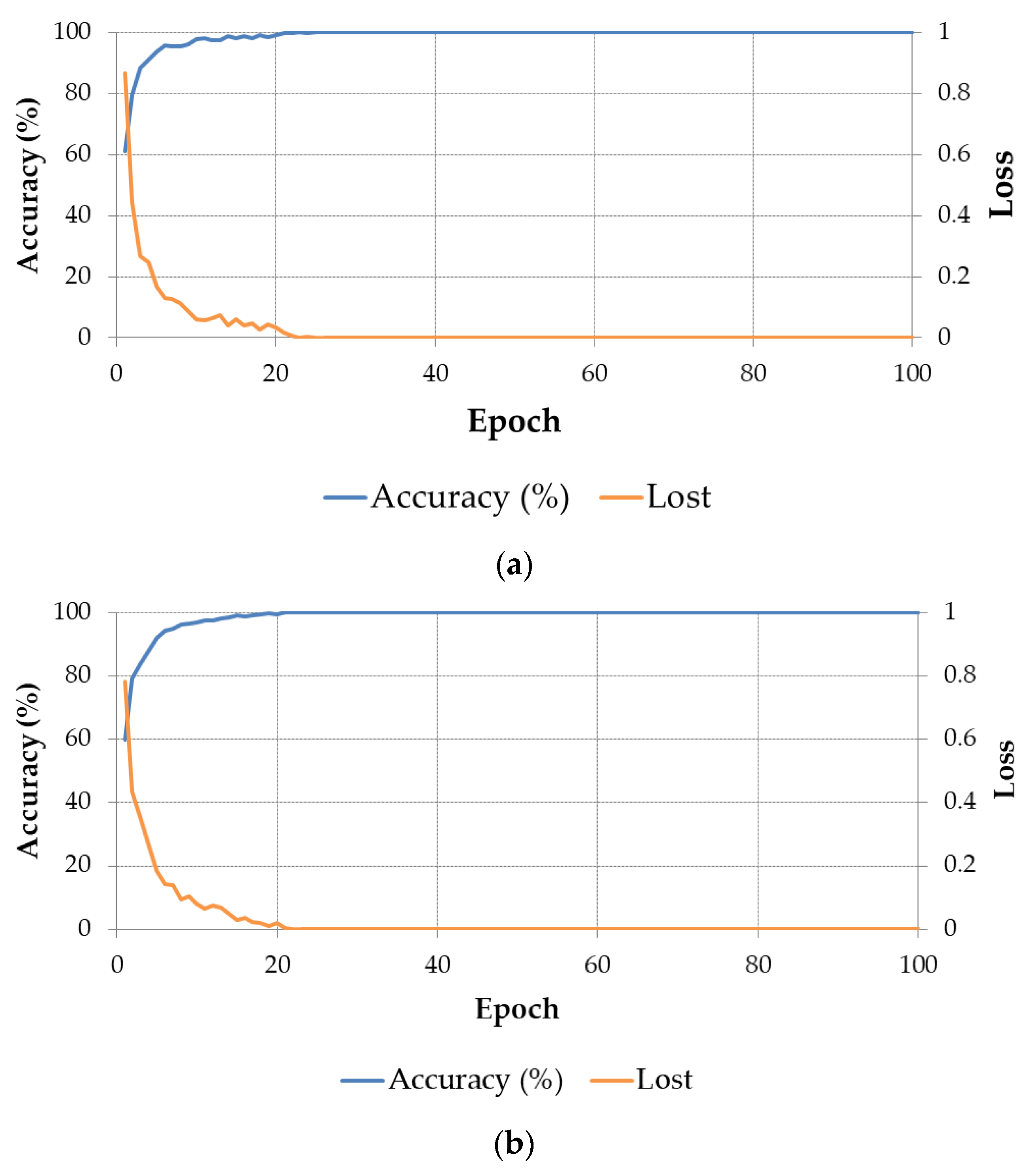Figure 7 shows the graphs of accuracy and batch loss of the training process on the two subsets of training data in the two-fold cross-validation method.

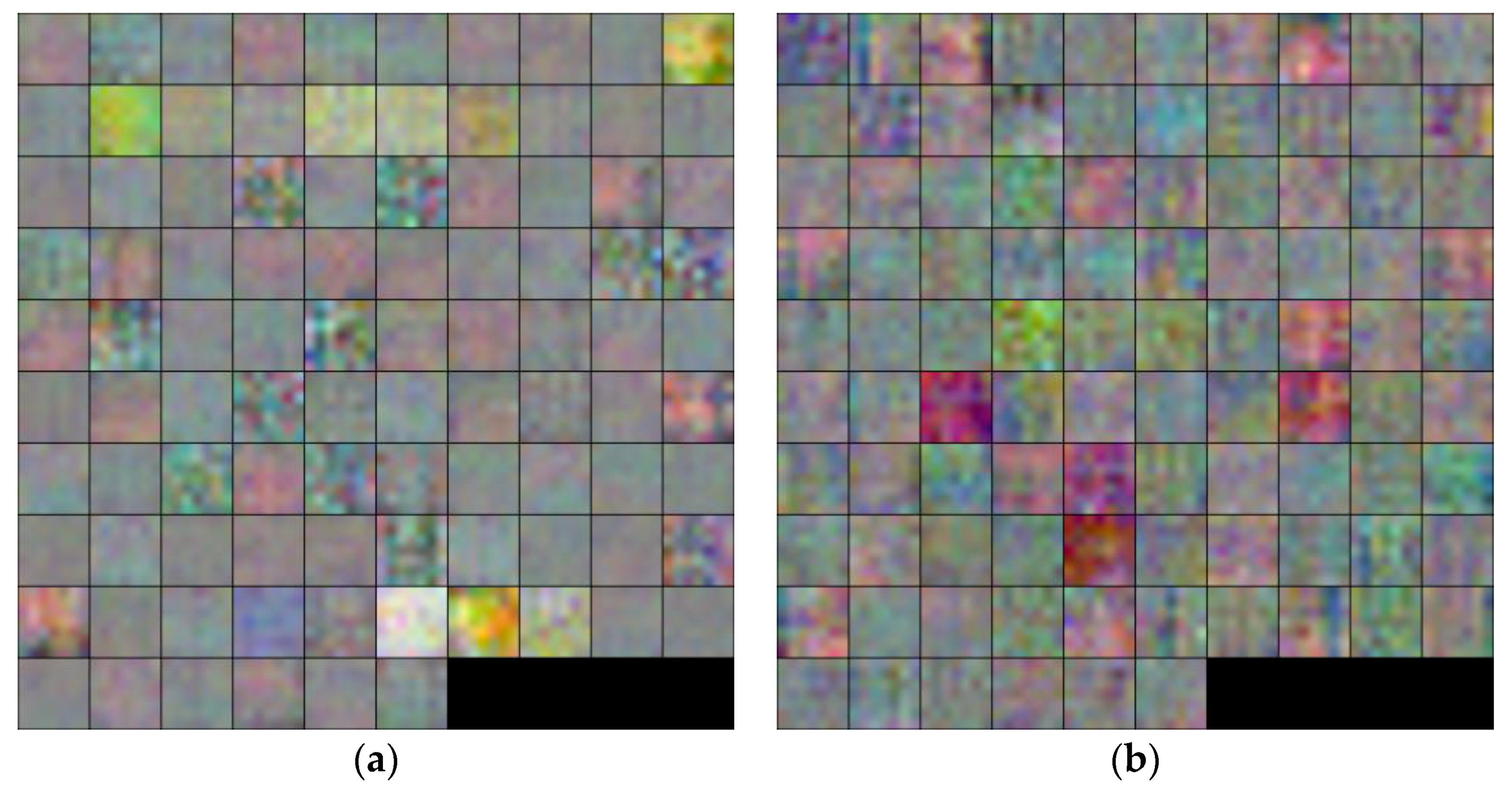
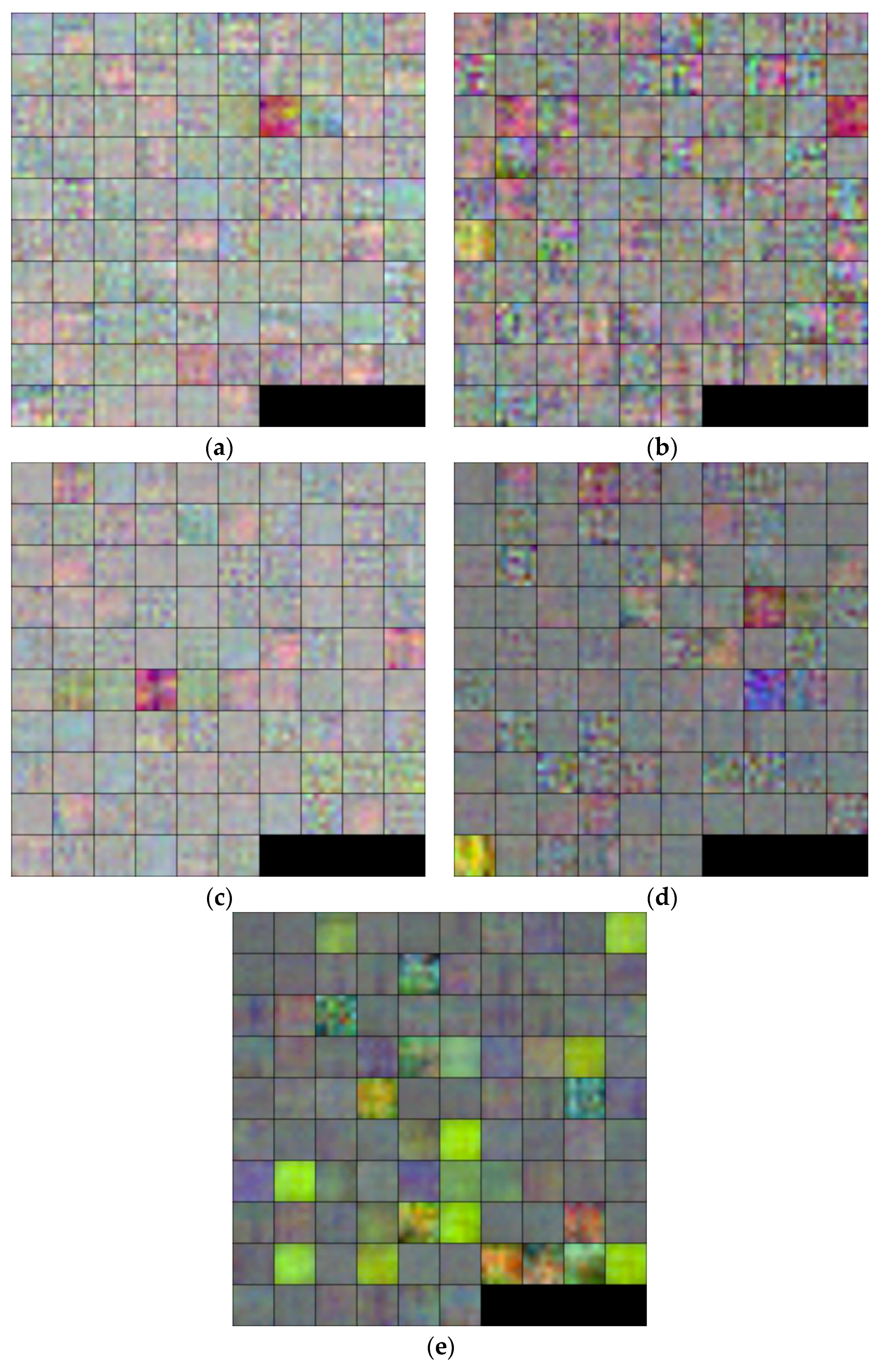
Figure 8 shows the trained filters in the first convolutional layer (L1) of the CNN models obtained by two training trials of the two-fold cross validation. The filters in the first layers were trained to extract the important low-, mid- and high-frequency features that reflect the fitness characteristics of a banknote on all the input image channels. Each filter in Figure 8 was resized from 7 × 7 × 3 pixels, as shown in Table 2, to five times larger, and scaled from the original real pixel values to the range of 0–255 by integer for visualization.

5.3. Testing of Proposed Method and Comparative Experiments

In the subsequent experiments, we performed the measurement of the classification accuracy on the remaining subsets against the training sets of the multinational banknote database. From the accuracies obtained by the two testing trials, we calculated the average accuracy as the ratio of the total accurately classified cases of the two subsets, and the total number of samples in the database [2,17]. In

Table 4. Confusion matrix of the testing results on the multinational banknote fitness database using the proposed method. The first testing results and second testing results mean the results of the testing on the first and second subsets of banknotes with the trained CNN models using the alternative subsets in the two-fold cross-validation method, respectively (unit: %).

First Testing Results		Classification Results
		Case 1–Fit	Case 1–Normal	Case 1–Unfit	Case 2–Fit	Case 2–Unfit
Desired Outputs	Case 1–Fit	99.805	0.195	0	0	0
	Case 1–Normal	0.470	99.177	0.353	0	0
	Case 1–Unfit	0	0.330	99.670	0	0
	Case 2–Fit	0	0	0	96.906	3.094
	Case 2–Unfit	0	0	0	39.175	60.825
Second Testing Results		Classification Results
		Case 1–Fit	Case 1–Normal	Case 1–Unfit	Case 2–Fit	Case 2–Unfit
Desired Outputs	Case 1–Fit	99.715	0.285	0	0	0
	Case 1–Normal	0.275	99.294	0.431	0	0
	Case 1–Unfit	0	0.693	99.307	0	0
	Case 2–Fit	0	0	0	98.517	1.483
	Case 2–Unfit	0	0	0	32.787	67.213
Average Accuracy		98.977

, we show the confusion matrices of the classification accuracy of the experimental results using the proposed CNN-based method with two-fold cross validation on the multinational banknote fitness database.

As shown in Table 4, the overall testing accuracy of the proposed method on the experimental database with merged currency types, denominations, and input directions of the banknotes is nearly 99%. These results proved that the proposed CNN-based method yields good fitness classification performance with the conditions of the multinational banknote dataset.

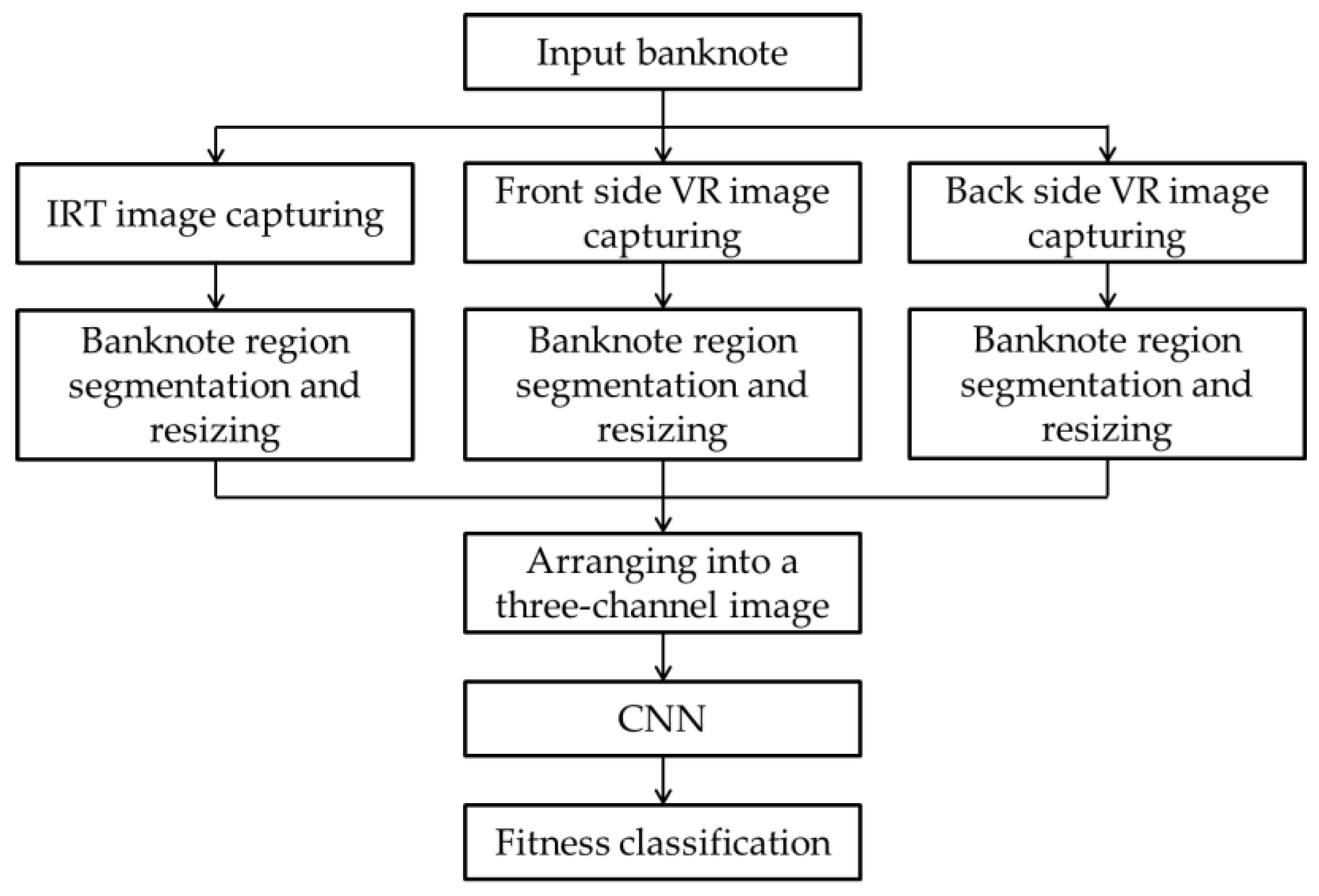
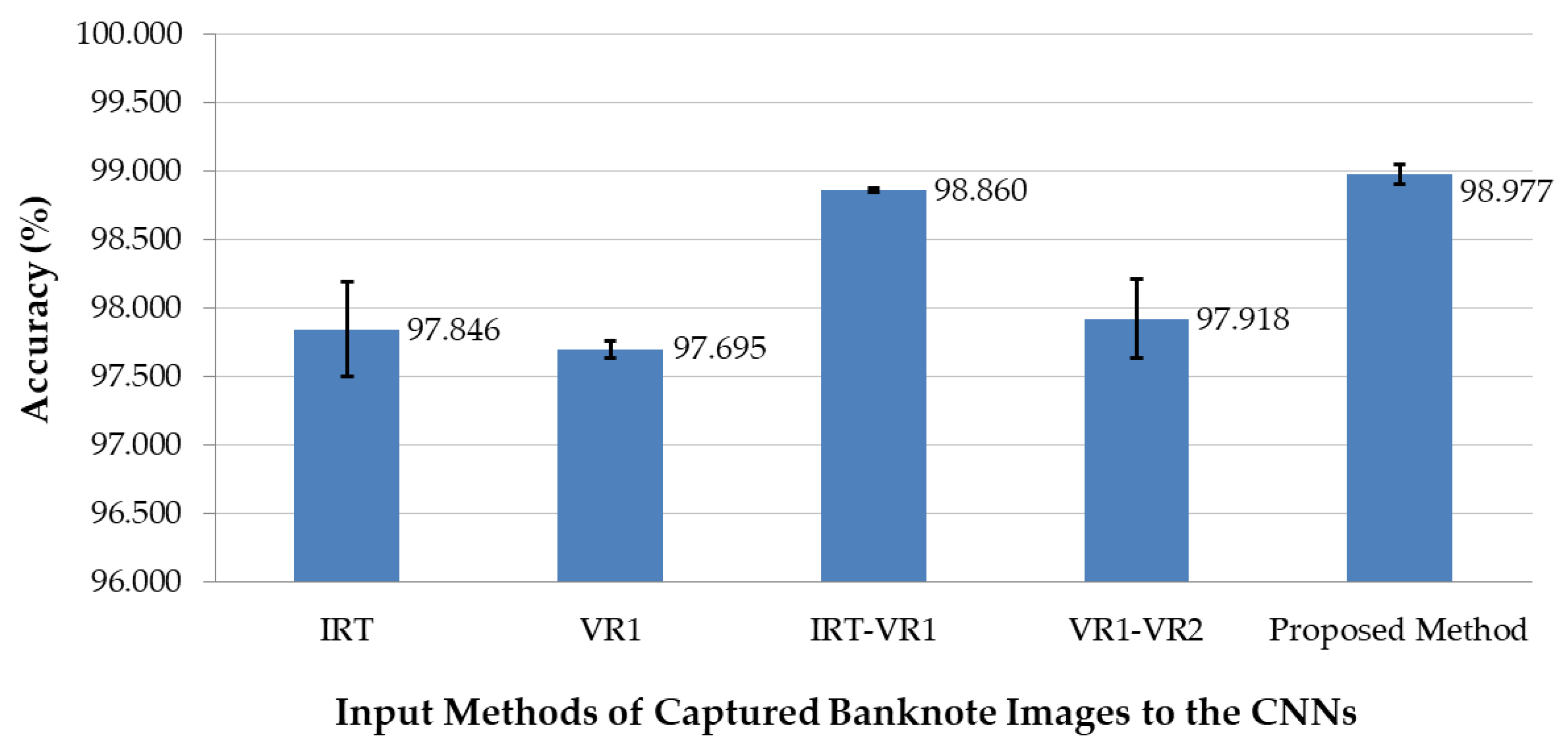
In the proposed method, we used the combination of images captured by various sensors per input banknote, in which one IRT and two VR images were used. In the next experiments, we investigated the optimality of the possible combinations of the captured images per banknote for inputting to the CNN models, as well as the effect of each type of image on the classification of the banknote fitness. Five cases were considered: using IRT images only (denoted by IRT), using VR images captured from the front side only (denoted by VR1), using two-channel input images of IRT and front side VR images (denoted by IRT-VR1), using two-channel input images of two VR images (denoted by VR1-VR2), and using three-channel input images of IRT and two VR images (the proposed method). In the multinational banknote database, the USD dataset consists of only one IRT and one VR image captured from the front side; therefore, the combination of IRT and reverse side VR images, which might be considered as IRT-VR2, is not considered. In the case of VR1-VR2, for the USD banknotes in the dataset, the VR image was duplicated into the two channels of the input image. We also used the CNN structure similar to the two-fold cross-validation for these comparative experiments. The results are shown in Figure 9 with the average classification accuracy for each case of input image to the CNNs.

Among the methods for inputting banknotes to the CNNs, the proposed method of using the three-channel input comprising all the captured images yielded the best accuracy, because it can fully utilize the available captured information of the banknote for fitness classification, as shown in Figure 9. Furthermore, Figure 9 shows that the IRT images of the banknote reflect the most fitness information, expressed by the high classification accuracy in the cases that present IRT images.

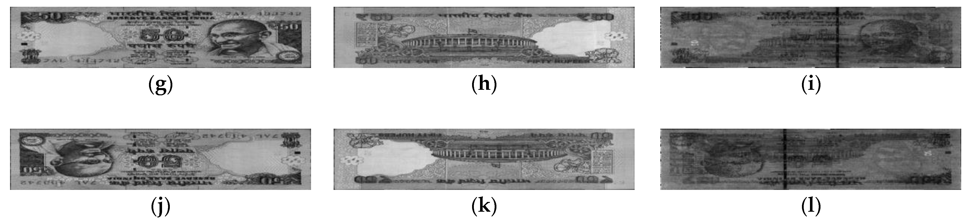
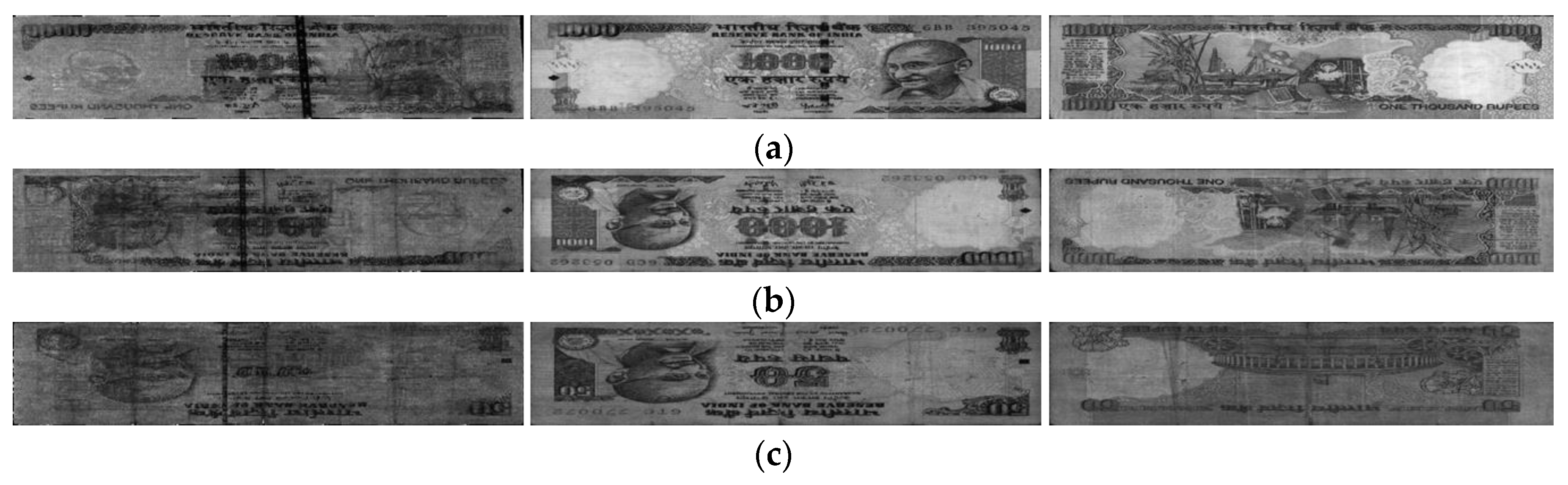
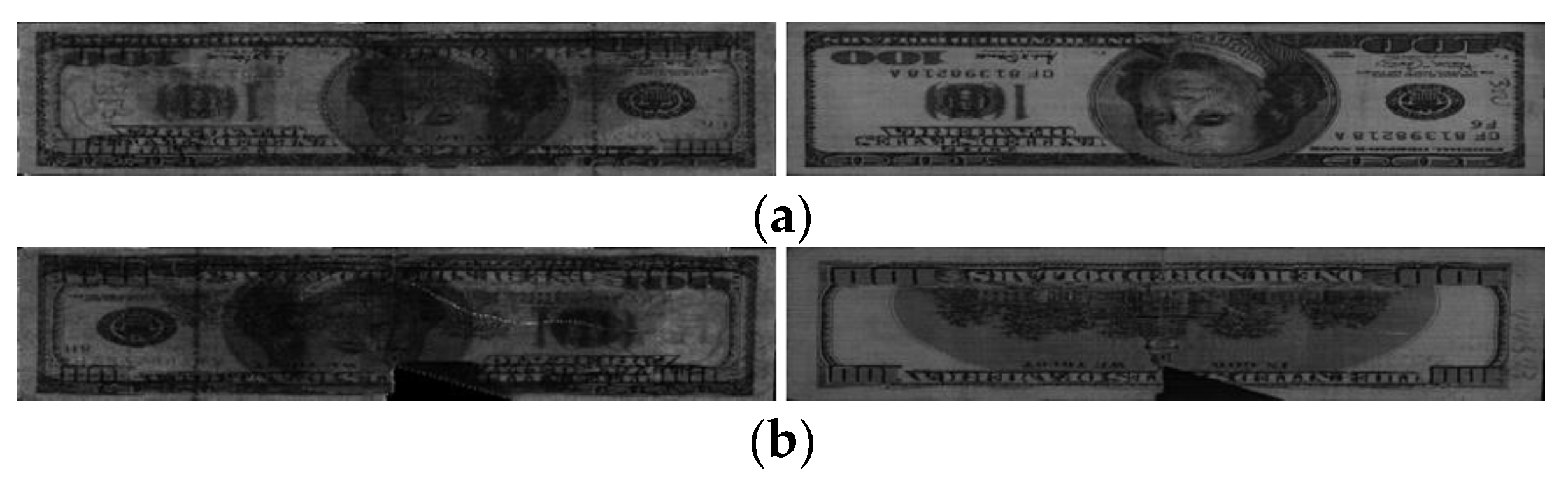
The examples of the correctly classified cases by our proposed method are shown in Figure 10, including the captured images of the banknotes from the three national currencies of the database. Figure 10 shows that the fitness levels in these examples are more clearly distinguished for the INR banknotes than those for KRW and USD. However, the IRT images of banknotes from different fitness levels are slightly more distinguishable than the VR images. This results in the relative high classification effect of the IRT images, as shown in the experimental results of Figure 9. To adapt to the multinational banknote fitness system, the VR image of USD, or the Case 2 fitness, need to be duplicated to form the three-channel input image. This leads to insufficient information for fitness classification in this case, and results in the high error rate in the Case 2 fitness levels.

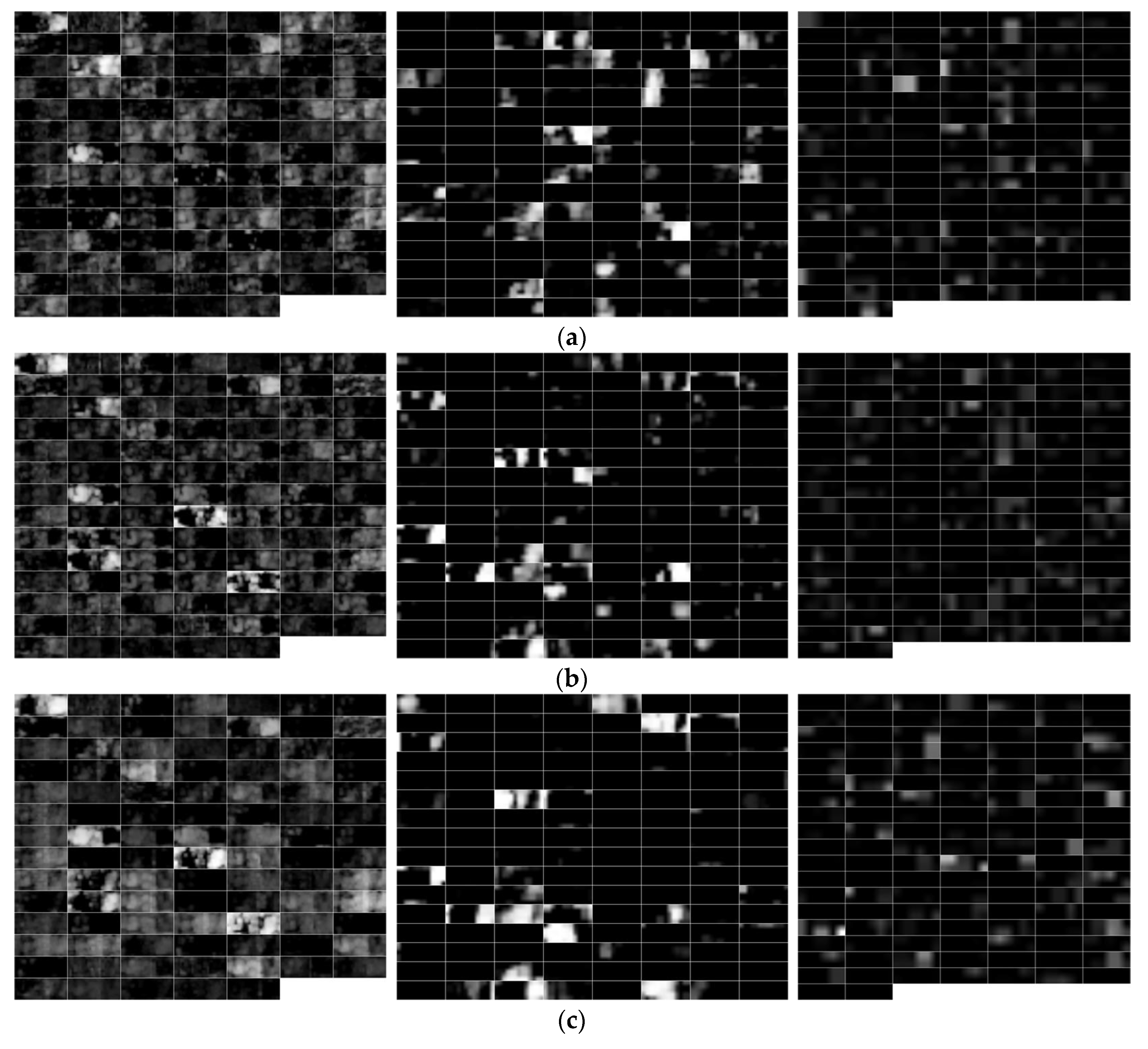
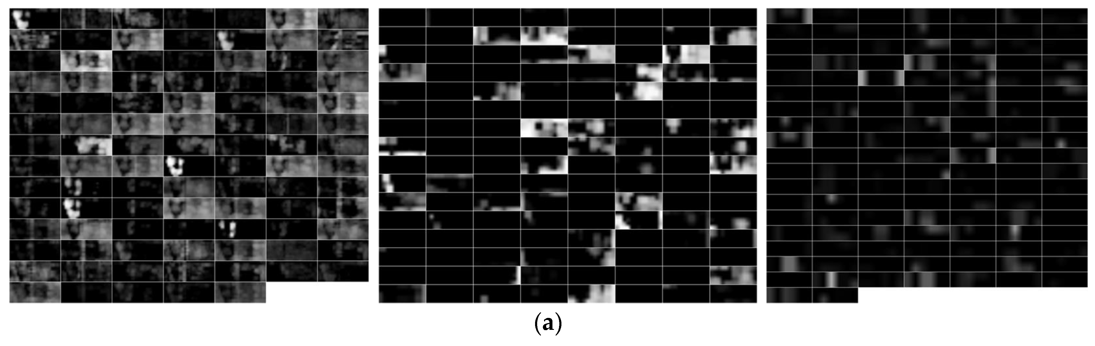
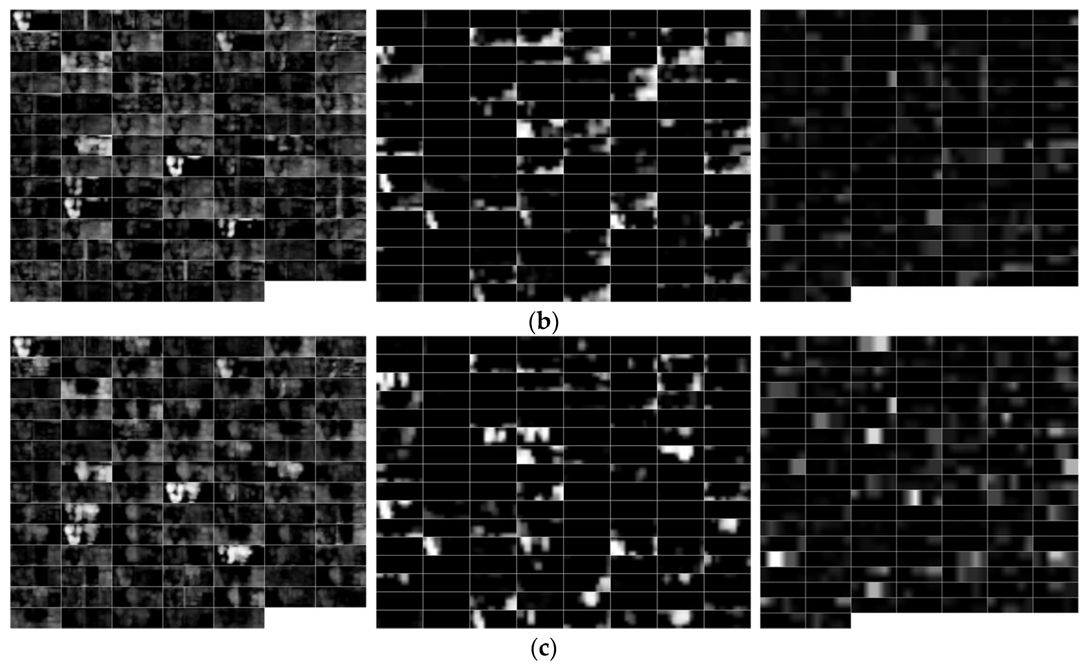
In Figure 11, Figure 12 and Figure 13, we visualize the examples of feature maps at the outputs of the pooling layers in the CNN structure for the genuine acceptance cases shown in Figure 10. There are three max pooling layers in the convolutional layers of L1, L2 and L5. At the output of these pooling layers of L1, L2 and L5, the numbers of feature maps’ channels are 96, 128 and 128, respectively, as shown in Table 2. By visualizing the output feature maps, we can see in Figure 11, Figure 12 and Figure 13 that the extracted features become more distinguishable over the stages of the convolutional layers among banknotes of the same national currency with different fitness classes. Banknote images responded differently to the filters of the first convolutional layer, and the output features of this L1 layer consist of many minor details, as shown in the left images of Figure 11, Figure 12 and Figure 13. However, as the banknote features pass through the stages of the convolutional networks from L1 to L5, the noises are gradually reduced, and only the classification features are maintained before being input to the successive fully connected layers. In the Case 1 fitness examples of Figure 11 and Figure 12, the output features at the last layer (L5) consist of the patterns that their noticeability reduces from unfit to normal to fit input banknotes, because the high-pass filters in the first L1 layers, which are visualized in Figure 8, tend to have more response to the details of the damage on the unfit banknote images than those on the normal and fit banknotes. These responses are maintained through max pooling layers to the last layers of the feature extraction part of the CNN. With the Case 2 fitness of USD, fitness levels of fit and unfit tend to be classified according to the brightness of the banknote images, since unfit banknote features at L5 have lower pixel values than that of the fit banknote, as shown in Figure 13.

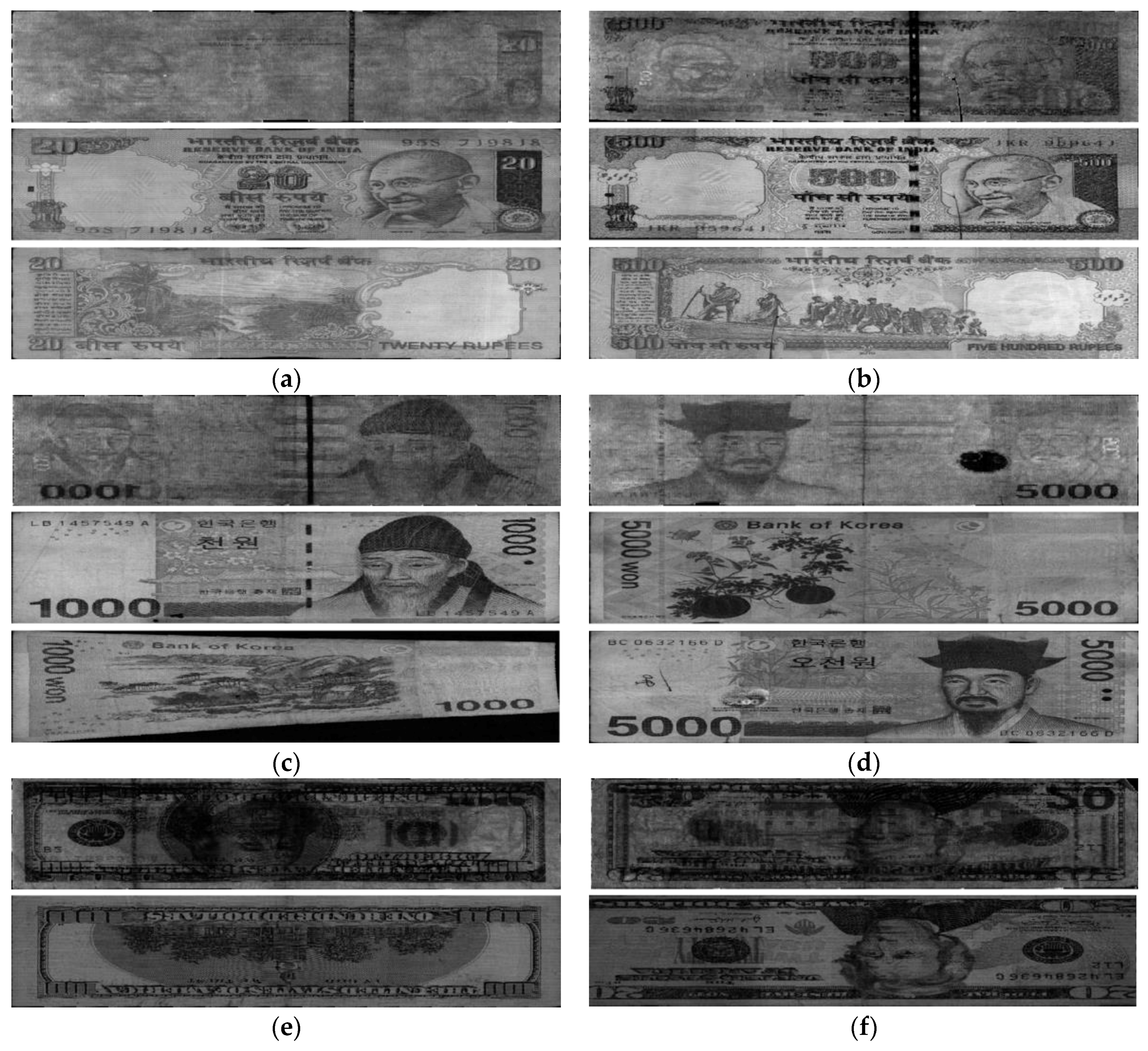
Figure 14 shows the examples of error cases that occurred in the testing process for each case of fitness levels. In some cases, the banknote region segmentation did not operate correctly, as shown in Figure 14c,f. Consequently, the classification results were affected. The fit INR banknote in Figure 14a was misclassified to normal, because it contained a reverse side VR image with slightly low contrast, and soiling on the upper part, which was visible but not as clear in the IRT and front side VR images. The soiling in the lower part of the VR image is also the reason for the fit banknote in Figure 14e to be incorrectly recognized as unfit. In the case of normal fitness banknote in Figure 14b, the brightness of the banknote images were not highly different from the fit banknotes; meanwhile, the tearing near the middle of the banknote was not clearly visible when being resized to be input to the CNN. The misclassification to unfit shown in Figure 14d is a KRW banknote with normal fitness with a small tearing part that is visible by the IRT image, and the handwritten mark on the opposite side of the banknote is captured by the VR sensor.

To make a further comparison with an equal number of fitness levels, we conducted the experiments of multinational banknote fitness classification with the two fitness levels of fit and unfit on the three currency types (USD, KRW, and INR) in the database. Since the fitness levels of the banknotes in the database were determined by human experts based on the densitometer measurement values [10], it is difficult to manually and subjectively reassign an additional level of normal for USD banknotes, as well as reassign the normal banknotes of INR and KRW into fit and unfit classes. As a result, we considered the experiments with the two fitness levels of fit and unfit cases. With the normal banknotes excluded from the INR and KRW datasets, we modified the CNN structure to have two outputs, corresponding to the two classes of fit and unfit of the three national currencies’ datasets. Experimental results of two-fold cross-validation of the two fitness levels classification for multiple currencies of INR, KRW and USD using the proposed CNN-based method are shown in

Table 5. Confusion matrix of the testing results on the multinational banknote fitness database with two fitness levels using the proposed method. The first testing and second testing mean the same as those in Table 4 (unit: %).

First Testing Results		Classification Results
		Fit	Unfit
Desired Outputs	Fit	99.686	0.314
	Unfit	1.987	98.013
Second Testing Results		Classification Results
		Fit	Unfit
Desired Outputs	Fit	99.685	0.315
	Unfit	1.570	98.430
Average Accuracy		99.237

in the form of confusion matrices. In

Table 6. Classification accuracy on each national currency dataset with two fitness levels of fit and unfit using the proposed method. The first testing and second testing mean the same as those in Table 4 (unit: %).

Currency Type	First Testing Results	Second Testing Results	Average Accuracy
INR	100	99.971	99.985
KRW	99.985	100	99.992
USD	93.679	94.604	94.138

, we show the experimental results with average accuracy of each testing phase and overall testing results in Table 5 separately for each national currency.

It can be seen from Table 6 that the classification accuracies of INR and KRW were nearly 100% and the performance in the case of the USD dataset is the lowest among the three national currencies. The reason for the experimental results can be explained as follows. The data of the three fitness levels exists for the original INR and KRW databases. Therefore, without the data of normal banknotes from these databases, the possibility of overlap between the two classes of fit and unfit is lower than that among the three classes of fit, normal, and unfit. Whereas, the original USD dataset has two fitness levels, and the consequent possibility of overlap between classes is still maintained. Moreover, the third channel of input image in the case of USD is the duplication of the VR image in the second channel to adapt to the three-channel input of the CNN structure, resulting in the disparity of the fitness information in the input data between USD banknotes and the banknotes of the remaining currencies. This causes the lower accuracy in the case of USD compared to INR and KRW.

For confirming the generalization of the results of the proposed method, we conducted the additional experiments with a five-fold cross-validation method. That is, the database was randomly divided into five subsets, in which four subsets were used for training and the remainder was used for testing. These processes of training and testing are repeated five times with the alternated subsets, and we calculated the average testing accuracy. Figure 15 shows the visualized filters in the first convolutional layer (L1) of the CNN models obtained by five training experiments. The visualization method is similar to that of Figure 8. The confusion matrices of the experimental results with five-fold cross-validation using the proposed method are shown in

Table 7. Confusion matrix of the testing results on the multinational banknote fitness database using the proposed method. The first, second, third, fourth, and fifth testing results mean the results of the testing on the first, second, third, fourth and fifth subsets of banknotes, with the trained CNN models using the remaining four subsets in each case in the five-fold cross-validation method, respectively (unit: %).

First Testing Results		Classification Results
		Case 1–Fit	Case 1–Normal	Case 1–Unfit	Case 2–Fit	Case 2–Unfit
Desired Outputs	Case 1–Fit	99.962	0.038	0	0	0
	Case 1–Normal	0.196	99.559	0.245	0	0
	Case 1–Unfit	0	0.226	99.774	0	0
	Case 2–Fit	0	0	0	99.020	0.980
	Case 2–Unfit	0	0	0	28.767	71.233
Second Testing Results		Classification Results
		Case 1–Fit	Case 1–Normal	Case 1–Unfit	Case 2–Fit	Case 2–Unfit
Desired Outputs	Case 1–Fit	99.850	0.150	0	0	0
	Case 1–Normal	0.049	99.706	0.245	0	0
	Case 1–Unfit	0	0.376	99.624	0	0
	Case 2–Fit	0	0	0	99.031	0.969
	Case 2–Unfit	0	0	0	18.421	81.579
Third Testing Results		Classification Results
		Case 1–Fit	Case 1–Normal	Case 1–Unfit	Case 2–Fit	Case 2–Unfit
Desired Outputs	Case 1–Fit	99.925	0.075	0	0	0
	Case 1–Normal	0.196	99.706	0.098	0	0
	Case 1–Unfit	0	0.526	99.474	0	0
	Case 2–Fit	0	0	0	97.868	2.132
	Case 2–Unfit	0	0	0	14.474	85.526
Fourth Testing Results		Classification Results
		Case 1–Fit	Case 1–Normal	Case 1–Unfit	Case 2–Fit	Case 2–Unfit
Desired Outputs	Case 1–Fit	99.700	0.300	0	0	0
	Case 1–Normal	0.245	99.412	0.343	0	0
	Case 1–Unfit	0	0.225	99.775	0	0
	Case 2–Fit	0	0	0	97.674	2.326
	Case 2–Unfit	0	0	0	13.158	86.842
Fifth Testing Results		Classification Results
		Case 1–Fit	Case 1–Normal	Case 1–Unfit	Case 2–Fit	Case 2–Unfit
Desired Outputs	Case 1–Fit	98.951	1.049	0	0	0
	Case 1–Normal	1.274	97.844	0.882	0	0
	Case 1–Unfit	0	1.503	98.497	0	0
	Case 2–Fit	0	0	0	94.767	5.233
	Case 2–Unfit	0	0	0	13.158	86.842
Average Accuracy		99.143

.

It can be seen from Table 7 that the average classification accuracy of the five-fold cross-validation was slightly higher than that of the two-fold cross-validation using the proposed method, as shown in Table 4, owing to the more intensive training tasks in the five-fold cross-validation compared to the two-fold cross-validation method.

In order to compare our method to the more complex network, we conducted comparative experiments with the ResNet model [30]. In these experiments, we used the pretrained ResNet-50 model that was trained on the ImageNet database on MATLAB [31] and conducted transfer learning [32] with the following parameters: the first half number of the layers of ResNet-50 model is frozen while training, the number of training epochs was 10, and the learning rate was 0.001. The experimental results of two-fold cross-validation on the multinational banknote fitness database using ResNet-50 CNN structure are shown in

Table 8. Confusion matrix of the testing results on the multinational banknote fitness database using the proposed method. The first testing and second testing mean the same as those in Table 4 (unit: %).

First Testing Results		Classification Results
		Case 1–Fit	Case 1–Normal	Case 1–Unfit	Case 2–Fit	Case 2–Unfit
Desired Outputs	Case 1–Fit	98.397	1.603	0	0	0
	Case 1–Normal	3.839	92.656	3.506	0	0
	Case 1–Unfit	0	1.382	98.618	0	0
	Case 2–Fit	0	0	0	97.525	2.475
	Case 2–Unfit	0	0	0	47.938	52.062
Second Testing Results		Classification Results
		Case 1–Fit	Case 1–Normal	Case 1–Unfit	Case 2–Fit	Case 2–Unfit
Desired Outputs	Case 1–Fit	98.364	1.636	0	0	0
	Case 1–Normal	3.471	93.254	3.275	0	0
	Case 1–Unfit	0	2.048	97.952	0	0
	Case 2–Fit	0	0	0	97.892	2.108
	Case 2–Unfit	0	0	0	39.891	60.109
Average Accuracy		96.156

in the form of confusion matrices.

It can be seen from Table 8 that the results when using ResNet-50 were not as good as those of the proposed method in terms of lower average classification accuracy. This can be explained by the method for training the network models between the two methods. The ResNet model was pretrained with the ImageNet database, and we applied transfer learning on this model with the first half number of the layers frozen to reduce training time. Meanwhile, for the proposed CNN structure, we conducted training from scratch by our banknote image dataset, as the number of parameters is smaller than that of the ResNet model. As a result, the filters in the early layers of our proposed model are able to respond and select the details on banknote images that reflect the fitness characteristic of the banknote, such as stains, tearing or other damage. The overall classification accuracy was higher when using the proposed method than using the ResNet model.

We also experimentally compared our proposed method to previous studies [2,7,9]. The two-fold cross-validation method was also adopted in these comparative experiments. In the method proposed in [2], the grayscale VR images of banknotes were used for the fitness classification by the CNN. This can be considered as equivalent to the VR1 experiment mentioned above. For the experiments using the method in [7], we extracted the histogram features from the grayscale VR images of the banknotes and classified the fitness levels using a multilayered perceptron (MLP) network with 95 nodes in the input and hidden layers. Referring to [9], we located the ROIs on the VR banknote images, performed Daubechies wavelet decomposition on the ROIs, and calculated the mean and standard variation values of the wavelet-transformed sub-bands. The means and standard variations were selected as the features to be classified for fitness levels by the SVM. The number of fitness classes in these three comparative experiments was maintained to that of the proposed method; consequently, we used the one-against-all training strategy for the SVM classifiers in the implementation of [9]. For the comparative experiments using the DWT and SVM method [9], the assumption of the prior knowledge of the currency type, denomination, and input direction of the banknote is required, as the ROI’s positions are different among the types of banknote images; meanwhile, in the cases of [2,7], we could conduct the comparative experiments with the multinational currency condition. The experiments with the previous fitness classification method were implemented in MATLAB [33,34]. 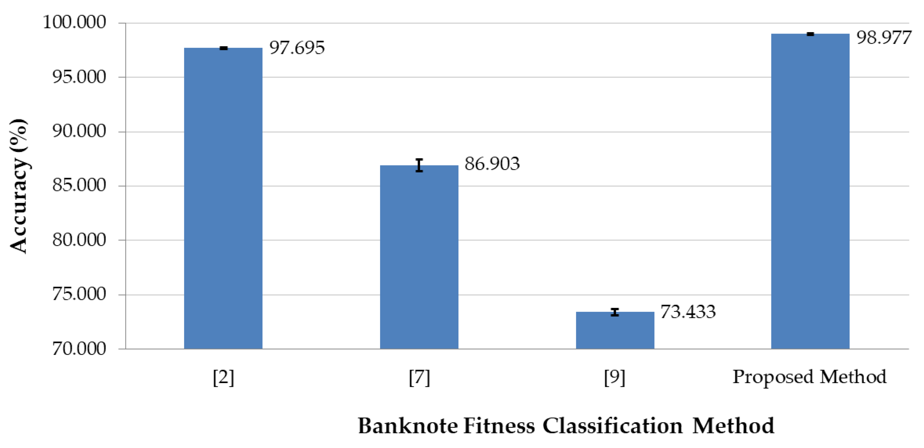Figure 16 shows the comparative experimental results of the proposed method to the previous study with the average classification accuracies of the two-fold cross-validation method.

As the method proposed in [9] required the pre-classification of denomination and input direction of banknote images, we implemented the experiments using this DWT and SVM-based method with two-fold cross-validation separately on each type of banknote image. As a result, the classification accuracies were calculated separately according to the currency types, denominations and input directions of banknotes, and shown in

Table 9. Comparison of classification accuracies by our proposed fitness classification method and the previous methods on each currency’s denomination and input direction. The first testing and second testing mean the same as those in Table 4 (unit: %). Denom = denomination. Dir = direction. Avg. Acc. = average accuracy.

Denom.	Dir.	Method Based on 1-Channel VR Image and CNN [2]			Method Based on Grayscale Histogram and MLP [7]			Method Based on DWT and SVM [9]			Proposed Method
		First Testing	Second Testing	Avg. Acc.	First Testing	Second Testing	Avg. Acc.	First Testing	Second Testing	Avg. Acc.	First Testing	Second Testing	Avg. Acc.
INR10	A	100	100	100	97.835	96.647	97.241	91.339	89.941	90.640	100	98.619	99.310
	B	100	100	100	97.292	98.450	97.870	91.489	90.892	91.191	100	98.643	99.322
INR20	A	100	99.718	99.860	85.434	90.986	88.202	85.994	84.789	85.393	99.720	100	99.860
	B	100	99.713	99.857	91.714	89.112	90.415	87.143	85.673	86.409	100	99.713	99.857
INR50	A	100	100	100	92.440	93.772	93.103	93.471	93.772	93.621	100	100	100
	B	100	99.654	99.828	95.533	91.696	93.621	89.347	91.695	90.517	100	100	100
INR100	A	99.623	99.244	99.434	96.101	94.836	95.469	90.566	92.191	91.378	99.623	100	99.811
	B	99.875	100	99.937	95.614	96.236	95.925	89.975	90.088	90.031	99.875	99.875	99.875
INR500	A	99.591	99.589	99.590	82.618	85.421	84.016	88.344	86.653	87.500	99.591	99.589	99.590
	B	99.596	99.594	99.595	84.242	81.339	82.794	85.050	86.410	85.729	99.394	100	99.696
INR1000	A	100	99.587	99.794	86.831	86.364	86.598	76.955	76.859	76.907	100	100	100
	B	100	100	100	87.500	85.772	86.640	79.839	79.268	79.555	99.194	99.593	99.393
KRW1000	A	98.676	96.729	97.703	84.289	80.990	82.641	78.376	81.609	79.991	99.382	99.558	99.470
	B	98.722	97.743	98.232	88.421	87.359	87.890	79.323	77.953	78.639	99.549	99.549	99.549
	C	96.438	96.257	96.347	87.088	82.709	84.900	51.291	49.020	50.156	99.020	98.930	98.976
	D	97.033	96.681	96.857	87.696	88.559	88.127	60.559	60.175	60.367	99.389	99.651	99.520
KRW5000	A	98.487	97.610	98.049	84.236	82.311	83.274	81.529	82.390	81.959	99.522	98.884	99.204
	B	98.348	98.348	98.348	83.934	82.132	83.033	79.054	79.129	79.092	99.625	99.625	99.625
	C	98.719	98.205	98.462	84.458	81.538	82.999	71.050	72.479	71.764	99.744	99.487	99.616
	D	97.738	97.896	97.817	82.472	83.172	82.821	76.737	77.184	76.960	99.273	99.434	99.353
USD5	A	60.526	75.000	67.568	63.158	72.222	67.568	81.579	83.333	82.432	84.211	94.444	89.189
	B	75.610	66.667	71.250	63.415	61.538	62.500	78.049	74.359	76.250	85.366	97.436	91.250
	C	77.143	79.412	78.261	74.286	67.647	71.014	82.857	76.471	79.710	85.714	91.176	88.406
	D	81.818	84.375	83.077	66.667	75.000	70.769	75.758	71.875	73.846	90.909	90.625	90.769
USD10	A	98.333	100	99.160	86.667	93.220	89.916	98.333	100	99.160	95.000	98.305	96.639
	B	73.016	75.806	74.400	80.952	80.645	80.800	80.952	70.968	76.000	90.476	83.871	87.200
	C	86.441	77.193	81.897	77.966	71.930	75.000	79.661	73.684	76.724	96.610	84.211	90.517
	D	87.037	90.566	88.785	75.926	71.698	73.832	72.222	73.585	72.897	96.296	84.906	90.654
USD20	A	92.063	93.548	92.800	84.127	83.871	84.000	93.651	93.548	93.600	93.651	95.161	94.400
	B	81.818	81.818	81.818	69.091	80.000	74.545	74.546	80.000	77.273	89.091	96.364	92.727
	C	82.692	94.118	88.350	80.769	82.353	81.553	90.385	92.157	91.262	92.308	98.039	95.146
	D	84.615	86.275	85.437	86.538	82.353	84.466	88.462	88.235	88.350	92.308	90.196	91.262
USD50	A	92.437	96.639	94.538	88.235	84.874	86.555	95.798	95.798	95.798	96.639	96.639	96.639
	B	79.646	95.495	87.500	78.761	87.387	83.036	92.035	92.793	92.411	92.035	93.694	92.857
	C	97.248	97.222	97.235	96.330	90.741	93.548	97.248	97.222	97.235	96.330	100	98.157
	D	97.222	97.170	97.196	95.370	94.340	94.860	95.370	96.226	95.794	94.444	98.113	96.262
USD100	A	93.750	93.636	93.694	92.857	90.909	91.892	91.071	91.818	91.441	91.964	97.273	94.595
	B	92.727	90.826	91.781	92.727	88.073	90.411	88.182	88.073	88.128	95.455	97.248	96.347
	C	93.519	94.393	93.953	87.037	88.785	87.907	88.889	86.916	87.907	88.889	97.196	93.023
	D	90.291	97.087	93.689	92.233	89.320	90.777	89.320	89.320	89.320	84.466	91.262	87.864
Avg. Acc.		97.695			86.903			79.252			98.977

for all the adopted methods. In the methods in [2,7] and the proposed method, the pre-classification of these categories was not required.

The experimental results in Figure 16 show that the proposed method outperformed the methods of the previous studies, and in most of the cases of banknote types in Table 9, the proposed method and the CNN-based method in [2] outperformed the other methods in terms of higher average classification accuracy with two-fold cross validation. The reason for the comparative experimental results can be explained as follows. The histogram-based method of [7] used only the brightness characteristic of the visible light banknote images, which were strongly affected by the illumination condition of the sensors, for the fitness levels determination. This consequently does not guarantee the reliability for the recognition of the other cases of degradation such as tearing or staining, which might occur sparsely on the banknote and are hardly represented by the brightness histogram characteristics. In the case of [9], banknote fitness was classified by the features extracted from the ROIs that are the blank areas on the banknote images. This method is not effective for cases where damage or staining occurs on other areas of the banknotes. The most accurate recognition cases were the CNN-based methods of [2] and the proposed method, in which the proposed method used the additional IRT images for the classification of the banknote fitness. The advantage of the CNN-based method is that both of the classifier’s parameters in the fully connected layers and the feature extraction stage’s parameters in the convolutional layers are trained with the training dataset. In addition, the proposed method used banknote images captured by various sensors of visible-light and near-infrared. Consequently, the appropriate features for the fitness classification of banknotes can be captured by the proposed system and extracted, as well as classified, by the CNN architecture to obtain the best accuracy, compared to the previous methods in the experiments shown in Figure 16.

6. Conclusions

In this study, we proposed a multinational banknote fitness classification method using IRT and two-sided VR images of the input banknote, and the CNN. The proposed method is designed to simultaneously classify the fitness of banknotes from three national currencies: INR, KRW, and USD. The fitness levels were mixed with three levels for the INR and KRW banknotes, and two levels for the USD banknotes. The experimental results (using two-fold cross validation in the combined banknote fitness database of INR, KRW, and USD banknote images), showed that our proposed method yielded good performance and outperformed the previous fitness classification method in terms of higher accuracy. For future work, we plan to combine the banknote fitness classification with the recognition of banknote type and denomination, as well as further study other problems related to banknote sorting, such as counterfeit detection and serial number recognition, using various architectures of the CNN. We also plan to study employing handcrafted features in combination with the CNN features of input banknote images for enhancing the performance of the banknote classification systems.

References

1. Lee, J.W.; Hong, H.G.; Kim, K.W.; Park, K.R. A Survey on Banknote Recognition Methods by Various Sensors. Sensors 2017, 17, 313. [Google Scholar] [CrossRef] [PubMed]
2. Pham, T.D.; Nguyen, D.T.; Kim, W.; Park, S.H.; Park, K.R. Deep Learning-Based Banknote Fitness Classification Using the Reflection Images by a Visible-Light One-Dimensional Line Image Sensor. Sensors 2018, 18, 472. [Google Scholar] [CrossRef] [PubMed]
3. Balke, P. From Fit to Unfit: How Banknotes Become Soiled. In Proceedings of the Fourth International Scientific and Practical Conference on Security Printing Watermark Conference, Rostov-on-Don, Russia, 21–23 June 2011. [Google Scholar]
4. Geusebroek, J.-M.; Markus, P.; Balke, P. Learning Banknote Fitness for Sorting. In Proceedings of the International Conference on Pattern Analysis and Intelligent Robotics, Putrajaya, Malaysia, 28–29 June 2011; pp. 41–46. [Google Scholar]
5. Balke, P.; Geusebroek, J.M.; Markus, P. BRAIN2—Machine Learning to Measure Banknote Fitness. In Proceedings of the Optical Document Security Conference, San Francisco, CA, USA, 18–20 January 2012. [Google Scholar]
6. Aoba, M.; Kikuchi, T.; Takefuji, Y. Euro Banknote Recognition System Using a Three-Layered Perceptron and RBF Networks. IPSJ Trans. Math. Model. Appl. 2003, 44, 99–109. [Google Scholar]
7. He, K.; Peng, S.; Li, S. A Classification Method for the Dirty Factor of Banknotes Based on Neural Network with Sine Basis Functions. In Proceedings of the International Conference on Intelligent Computation Technology and Automation, Changsha, China, 20–22 October 2008; pp. 159–162. [Google Scholar]
8. Sun, B.; Li, J. The Recognition of New and Old Banknotes Based on SVM. In Proceedings of the 2nd International Symposium on Intelligent Information Technology Application, Shanghai, China, 20–22 December 2008; pp. 95–98. [Google Scholar]
9. Pham, T.D.; Park, Y.H.; Kwon, S.Y.; Nguyen, D.T.; Vokhidov, H.; Park, K.R.; Jeong, D.S.; Yoon, S. Recognizing Banknote Fitness with a Visible Light One Dimensional Line Image Sensor. Sensors 2015, 15, 21016–21032. [Google Scholar] [CrossRef] [PubMed] [Green Version]
10. Kwon, S.Y.; Pham, T.D.; Park, K.R.; Jeong, D.S.; Yoon, S. Recognition of Banknote Fitness based on a Fuzzy System Using Visible Light Reflection and Near-Infrared Light Transmission Images. Sensors 2016, 16, 863. [Google Scholar] [CrossRef] [PubMed]
11. Lee, S.; Baek, S.; Choi, E.; Baek, Y.; Lee, C. Soiled Banknote Fitness Determination Based on Morphology and Otsu’s Thresholding. In Proceedings of the IEEE International Conference on Consumer Electronics, Las Vegas, NV, USA, 8–10 January 2017; pp. 450–451. [Google Scholar]
12. Khashman, A.; Sekeroglu, B. Multi-Banknote Identification Using a Single Neural Network. In Proceedings of the International Conference on Advanced Concepts for Intelligent Vision Systems, Antwerp, Belgium, 20–23 September 2005; pp. 123–129. [Google Scholar]
13. Takeda, F.; Nishikage, T.; Matsumoto, Y. Characteristics Extraction of Paper Currency Using Symmetrical Masks Optimized by GA and Neuro-Recognition of Multi-National Paper Currency. In Proceedings of the IEEE International Joint Conference on Neural Networks, Anchorage, AK, USA, 4–9 May 1998; pp. 634–639. [Google Scholar]
14. Youn, S.; Choi, E.; Baek, Y.; Lee, C. Efficient Multi-Currency Classification of CIS Banknotes. Neurocomputing 2015, 156, 22–32. [Google Scholar] [CrossRef]
15. Rahman, S.; Banik, P.; Naha, S. LDA based Paper Currency Recognition System Using Edge Histogram Descriptor. In Proceedings of the 17th International Conference on Computer and Information Technology, Dhaka, Bangladesh, 22–23 December 2014; pp. 326–331. [Google Scholar]
16. Hassanpour, H.; Farahabadi, P.M. Using Hidden Markov Models for Paper Currency Recognition. Expert Syst. Appl. 2009, 36, 10105–10111. [Google Scholar] [CrossRef]
17. Pham, T.D.; Lee, D.E.; Park, K.R. Multi-National Banknote Classification based on Visible-Light Line Sensor and Convolutional Neural Network. Sensors 2017, 17, 1595. [Google Scholar] [CrossRef] [PubMed]
18. Nanni, L.; Ghidoni, S.; Brahnam, S. Handcrafted vs. Non-Handcrafted Features for Computer Vision Classification. Pattern Recognit. 2017, 71, 158–172. [Google Scholar] [CrossRef]
19. Dongguk Fitness Database (DF-DB2) & CNN Model. Available online: http://dm.dgu.edu/link.html (accessed on 2 July 2018).
20. Newton. Available online: http://kisane.com/our-service/newton/ (accessed on 2 July 2018).
21. Krizhevsky, A.; Sutskever, I.; Hinton, G.E. ImageNet Classification with Deep Convolutional Neural Networks. In Proceedings of the Advances in Neural Information Processing Systems, Lake Tahoe, NV, USA, 3–8 December 2012. [Google Scholar]
22. Glorot, X.; Bordes, A.; Bengio, Y. Deep Sparse Rectifier Neural Networks. In Proceedings of the 14th International Conference on Artificial Intelligence and Statistics, Fort Lauderdale, FL, USA, 11–13 April 2011; pp. 315–323. [Google Scholar]
23. CS231n Convolutional Neural Networks for Visual Recognition. Available online: http://cs231n.github.io/convolutional-networks/ (accessed on 2 July 2018).
24. Srivastava, N.; Hinton, G.; Krizhevsky, A.; Sutskever, I.; Salakhutdinov, R. Dropout: A Simple Way to Prevent Neural Networks from Overfitting. J. Mach. Learn. Res. 2014, 15, 1929–1958. [Google Scholar]
25. Simonyan, K.; Zisserman, A. Very Deep Convolutional Networks for Large-Scale Image Recognition. In Proceedings of the 3rd International Conference on Learning Representations, San Diego, CA, USA, 7–9 May 2015; pp. 1–14. [Google Scholar]
26. Bishop, C.M. Pattern Recognition and Machine Learning; Springer: New York, NY, USA, 2006. [Google Scholar]
27. Deep Learning Training from Scratch—MATLAB & Simulink. Available online: https://www.mathworks.com/help/nnet/deep-learning-training-from-scratch.html (accessed on 2 July 2018).
28. Intel® CoreTM i7-3770K Processor (8 M Cache, up to 3.90 GHz) Product Specifications. Available online: https://ark.intel.com/products/65523/Intel-Core-i7-3770K-Processor-8M-Cache-up-to-3_90-GHz (accessed on 2 July 2018).
29. GTX 1070 Ti Gaming Graphics Card|NVIDIA GeForce. Available online: https://www.nvidia.com/en-us/geforce/products/10series/geforce-gtx-1070-ti/#specs (accessed on 2 July 2018).
30. He, K.; Zhang, X.; Ren, S.; Sun, J. Deep Residual Learning for Image Recognition. In Proceedings of the IEEE Conference on Computer Vision and Pattern Recognition, Las Vegas, NV, USA, 27–30 June 2016. [Google Scholar]
31. MathWorks Deep Learning Toolbox Team—MATLAB Central. Available online: https://www.mathworks.com/matlabcentral/profile/authors/8743315-mathworks-neural-network-toolbox-team (accessed on 17 September 2018).
32. Pretrained Convolutional Neural Networks—MATLAB & Simulink. Available online: https://www.mathworks.com/help/deeplearning/ug/pretrained-convolutional-neural networks.html (accessed on 17 September 2018).
33. Function Approximation and Clustering—MATLAB & Simulink. Available online: https://www.mathworks.com/help/nnet/function-approximation-and-clustering.html (accessed on 2 July 2018).
34. Support Vector Machine Classification—MATLAB & Simulink. Available online: https://www.mathworks.com/help/stats/support-vector-machine-classification.html (accessed on 2 July 2018).
Figure 1. Overall flowchart of the proposed method. IRT = infrared transmission.
Symmetry 10 00431 g001
Figure 2. Example of banknote images captured by the system in: forward direction with (a) front side VR image (A direction), (b) reverse side VR image (C direction) and (c) IRT image; backward direction with (d) front side VR image (B direction), (e) reverse side VR image (D direction) and (f) IRT image; (gl) are the corresponding banknote region segmented images from the original captured images in (af), respectively.
Symmetry 10 00431 g002aSymmetry 10 00431 g002b
Figure 3. Overall flowchart of the proposed method. L1–L5 = convolutional layers 1–5. F1–F3 = fully connected layers 1–3. ReLU = rectified linear unit. CCN = cross-channel normalization. Conv = two-dimensional (2-D) convolutional layers.
Symmetry 10 00431 g003
Figure 4. Examples of banknote images in the INR dataset: (a) fit; (b) normal; and (c) unfit banknotes. The images on the left, middle and right of each figure are the IRT image, the VR image captured from the same side with the IRT and the VR image captured from the opposite side of the input banknote, respectively.
Symmetry 10 00431 g004
Figure 5. Examples of banknote images in the KRW dataset: (a) fit; (b) normal; and (c) unfit banknotes. Images in each figure are arranged similarly as those in Figure 4.
Symmetry 10 00431 g005
Figure 6. Examples of banknote images in the USD dataset: (a) fit and (b) unfit banknotes. The images on the left and right of each figure are the IRT image and the VR image of the input banknote, respectively.
Symmetry 10 00431 g006
Figure 7. Convergence graphs with accuracy and batch loss of the training process on (a) first-fold and (b) second-fold subsets.
Symmetry 10 00431 g007
Figure 8. Visualization of the filter parameters in the first convolutional layer (L1) of the CNN model: (a) first-fold and (b) second-fold training results.
Symmetry 10 00431 g008
Figure 9. Comparative experimental results of fitness classification with various input methods of the captured banknote images to the CNNs.
Symmetry 10 00431 g009
Figure 10. Examples of correctly classified cases (genuine acceptance) by the proposed method of the (a) INR; (b) KRW and (c) USD datasets. In (a,b), from left to right are the IRT image and VR images of the front and reverse sides of the input banknote, respectively; and from the top down are the correctly classified Case 1–fit, Case 1–normal and Case 1–unfit banknotes, respectively. In (c), the left and right images are the IRT and VR images of the input USD banknote; and the upper and lower figures are the correctly classified Case 2–fit and Case 2–unfit banknotes, respectively.
Symmetry 10 00431 g010
Figure 11. Visualization of the feature maps at the output of the pooling layers in the CNN structure of the (a) fit, (b) normal and (c) unfit INR banknotes in the examples shown in Figure 10a. The images on the left, middle and right of each figure are the output features of the max pooling layers of the L1, L2 and L5 convolutional layers (as shown in Table 2), respectively.
Symmetry 10 00431 g011
Figure 12. Visualization of the feature maps at the output of the pooling layers in the CNN structure of the (a) fit, (b) normal and (c) unfit KRW banknotes in the examples shown in Figure 10b. The images in each figure are arranged similarly as those in Figure 11.
Symmetry 10 00431 g012aSymmetry 10 00431 g012b
Figure 13. Visualization of the feature maps at the output of the pooling layers in the CNN structure of the (a) fit and (b) unfit USD banknotes in the examples shown in Figure 10c. The images in each figure are arranged similarly as those in Figure 11.
Symmetry 10 00431 g013
Figure 14. Example of testing error cases by our method: (a) Case 1–fit banknote misclassified to Case 1–normal; (b) Case 1–normal banknote misclassified to Case 1–fit; (c) Case 1–unfit banknote misclassified to Case 1–normal; (d) Case 1–normal banknote misclassified to Case 1–unfit; (e) Case 2–fit banknote misclassified to Case 2–unfit; and (f) Case 2–unfit banknote misclassified to Case 2–fit. In each figure of (ad), the upper, middle and lower images are the IRT image and VR images of the front and reverse sides of the input banknote, respectively. In (e,f), the upper and lower images are the IRT image and VR image of the input banknote, respectively.
Symmetry 10 00431 g014
Figure 15. Visualization of the filter parameters in the first convolutional layer (L1) of the CNN model: (a) first-fold; (b) second-fold; (c) third-fold; (d) forth-fold; and (e) fifth-fold training results.
Symmetry 10 00431 g015
Figure 16. Comparative experimental results of the proposed method and the previous methods, including: method based on 1-channel VR images and CNN [2], method based on grayscale histogram and a multilayered perceptron (MLP) [7], and method based on DWT and SVM [9].
Symmetry 10 00431 g016