Classification of Landforms for Digital Soil Mapping in Urban Areas Using LiDAR Data Derived Terrain Attributes: A Case Study from Berlin, Germany


Department of Geography, Humboldt University of Berlin, 10099 Berlin, Germany
Land 2020, 9(9), 319; https://doi.org/10.3390/land9090319
Submission received: 9 August 2020
/
Revised: 6 September 2020
/
Accepted: 7 September 2020
/
Published: 9 September 2020
(This article belongs to the Section Land Planning and Landscape Architecture)
Abstract
:In this study, a knowledge-based fuzzy classification method was used to classify possible soil-landforms in urban areas based on analysis of morphometric parameters (terrain attributes) derived from digital elevation models (DEMs). A case study in the city area of Berlin was used to compare two different resolution DEMs in terms of their potential to find a specific relationship between landforms, soil types and the suitability of these DEMs for soil mapping. Almost all the topographic parameters were obtained from high-resolution light detection and ranging (LiDAR)-DEM (1 m) and Advanced Spaceborne Thermal Emission and Reflection Radiometer (ASTER)-DEM (30 m), which were used as thresholds for the classification of landforms in the selected study area with a total area of about 39.40 km2. The accuracy of both classifications was evaluated by comparing ground point samples as ground truth data with the classification results. The LiDAR-DEM based classification has shown promising results for classification of landforms into geomorphological (sub)categories in urban areas. This is indicated by an acceptable overall accuracy of 93%. While the classification based on ASTER-DEM showed an accuracy of 70%. The coarser ASTER-DEM based classification requires additional and more detailed information directly related to soil-forming factors to extract geomorphological parameters. The importance of using LiDAR-DEM classification was particularly evident when classifying landforms that have narrow spatial extent such as embankments and channel banks or when determining the general accuracy of landform boundaries such as crests and flat lands. However, this LiDAR-DEM classification has shown that there are categories of landforms that received a large proportion of the misclassifications such as terraced land and steep embankments in other parts of the study area due to the increased distance from the major rivers and the complex nature of these landforms. In contrast, the results of the ASTER-DEM based classification have shown that the ASTER-DEM cannot deal with small-scale spatial variation of soil and landforms due to the increasing human impacts on landscapes in urban areas. The application of the approach used to extract terrain parameters from the LiDAR-DEM and their use in classification of landforms has shown that it can support soil surveys that require a lot of time and resources for traditional soil mapping.
1. Introduction
In urban areas like the Berlin metropolitan area, soils have a variety of functions; however, they are a scarce property, which are not increasable. It is, therefore, necessary to reduce the spatial extent of urban areas in order to preserve soil functions. The conservation of soil structure and functions is essential for sustainable spatial and regional management as well as for maintaining the ecological functioning of an ecosystem in these areas [1,2,3]. This is particularly true for suburban areas where soil functions are severely constrained by urban growth conditions and topographic changes. In order to meet the legal requirements to maintain soil functions in accordance with the laws and regulations to soil protection, the detailed knowledge of soil mapping in urban areas is necessary. In addition, the quality of soil information acquired in one way or another plays a crucial role in determining the quality of the assessment of the suitability of soil functions and the reliability of the decisions associated with their use [3,4,5,6,7,8]. Therefore, digital mapping of the soil based on remote sensing data is an important and major source of information for the protection of soil functions and the management of land uses in urban areas [4].
Classical soil mapping cannot represent continuous changes in soil forms or soil types and cannot provide any information on the spatial variation of their individual characteristics. In addition, soil mapping is costly and time consuming, as it relies on intensive field surveys of soil [3,6,7,8,9]. Soil science, like many other fields within geography, can benefit from various remote sensing applications and improved geographic information system (GIS)-based analyzes for more efficient digital mapping of soil characteristics or soil types. This too ultimately contributes to the reduction of expensive fieldwork and subsequent analysis of physical and chemical soil properties in laboratory [4,9,10].
Due to automated classification techniques of soil parameters used in digital soil mapping, various topographic data can be obtained for soil distribution sites. With the development of these classification techniques, the role of topographical data in the digital mapping of the soil has increased. The processing and analysis of these spatial data according to specific rules allows for a quantitative prediction of the distribution of soil forms or soil types within landscapes [11,12]. There are several previous studies that dealt with the topic of digital mapping and survey of the soil [3,5,13,14,15,16,17,18,19,20,21,22,23].
Landforms are distinguished by their specific geometrical and topographical features [24]. Several methods have been developed that are based on topographic data analysis of relief using GIS and remote sensing techniques. This has helped to involve the pedological expertise and the use of geomorphometric data (digital terrain data) in order to classify the landforms and to map the soil at different target scales.
Digital elevation models (DEMs) have also been increasingly used in recent years in geomorphological and pedological research [25]. Thus, soil-landform classifications based on geomorphometric parameters (digital terrain data) derived from DEMs are important inputs to map soil and to predict soil characteristics [3,10,19,23,26,27,28,29,30,31,32]. From a geomorphological terms of view, quantified geomorphometric parameters can be understood as a continuous numeric description of the topographical surfaces or landforms. Thus, these landforms have specific topographic attributes, which allows topographically landscape to be distinguished from the other [33,34,35]. These features as morphological indicators are sensitive to spatially and temporally variable morphological processes and thus allow us to identify the physical, chemical and biological processes occurring in landscapes [34,35,36]. Thus, they give a quantitative description of landforms and soil variabilities.
In urban areas, the use of automated terrain analyses based on coarse DEMs and pixel-based classification techniques remains limited due to small-scale spatial variation of soil and landforms. So high-resolution DEMs derived from airborne light detection and ranging (LiDAR) could provide the necessary database for such analyses. However, new techniques will be needed to extract these data for use in soil and land classification in urban environments. There are several approaches developed for the extraction of morphometric parameters from different DEMs such as those using combination of morphometric parameters [37,38], fuzzy logic and unsupervised classification [6,7,32,36,37,38,39,40,41], supervised classification [42,43,44], probabilistic clustering algorithms [25,45,46], multivariate descriptive statistics [47,48,49] and double ternary diagram classification [50].
Landscapes in urban areas such as the Berlin metropolitan area have permanently changed by dense urban development and artificial transformations of natural surfaces. This made it very difficult to identify the original morphological or geological formations within urban areas [51]. This in turn makes geomorphological studies as well as soil studies in such areas difficult [52]. Therefore, this study investigates the possibility of classifying soil-landforms in urban areas based on analysis of geomorphometric features derived from very high-resolution LiDAR data. This classification applied in this study is based on an object-based image analysis approach (OBIA) instead of crisp classifications to extract morphometric parameters from DEMs. This classification is known as knowledge-based fuzzy classification [6,24]. This fuzzy classification has achieved better results than other classifications in organizing the segmentation of the land surface and the classification of object classes in a hierarchical manner [6,24]. Moreover, when classifying landforms in a specific geographical area, a trade-off between the delineation of landforms in this area and their classification is required [53]. This is possible in the OBIA approach [54]. The study also attempts to show whether it is sufficient correlation between landforms and the distribution of soil types in these areas as well as to show whether there are specific advantages for this classification by using LiDAR-DEM instead of other DEMs, which their use bases on the classification of pixels. This is done through a comparative geomorphometric analysis of LiDAR-DEM with a resolution of 1 m and ASTER-DEM with a resolution of 30 m. To analyze the LiDAR-DEM as compared to the ASTER-DEM for the soil-landforms classification, the study area was reduced to the area of the topographical chart Berlin–Rüdersdorf with a scale of 1:25,000. Such investigations on soil-landforms classification help to improve the understanding of the effect different factors on soil formation and distribution in the urban areas and to improve understanding of the soil-landscape relationship. All of which ultimately improve traditional surveys of soils in order to generate soil maps at a reasonable time and achieve better and more usable results.
2. Study Area
The test area is located in Köpenik district in the southeast of Berlin. Its borders range from 52°28′27.26″ N to 52°23′27.68″ N, and 13°45′43.19″ E to 13°38′15.45″ E. It covers an area of 39.40 km2 (Figure 1).
This area is located, as part of the city of Berlin, in a temperate climate zone with a humid continental climate with warm summers and cold winters [55,56]. The average annual temperature in Berlin is 9.4 °C and the average annual precipitation is about 566.4 mm. The warmest months are July and August, with average temperatures of 18.3 °C, while the coldest month is January, with an average temperature of −0.6 °C [56]. The altitude of the study area ranges from 30 m to 112 m above mean sea level. The elevations in the study area increase from the center, where the basin of Lake Müggelsee is located, to the sides in the north and south. The major land use and land cover are built-up areas (residential and commercial settlements and roads) 3.91 km2, green and open areas 9.17 km2, forest 24.15 km2 and water bodies 2.17 km2 [8].
Characteristic natural geomorphological units in the study area are the wide Berlin glacial valley, the melt water channels, the ground moraines plateaus, sand dunes, and lake and bog sediments of sand with mud and peat. During the glacial periods of Quaternary, different materials were deposited in these units, which include fine sand, middle sand, coarse sand to gravel, gravel with boulders and washed-out remains of ground moraine [51]. Therefore, the starting rock for soil formation, which reflects the natural-spatial differentiation of the study area, is decisive for the soil types (Figure 2). The sands of the Berlin glacial valley dominate mostly in the study area (57%). A large part of the study area is covered with wind-borne sand (20%), which is concentrated in the sand dunes of the study area. Sea chalks and valley sand are also found in the melt water channels and peat in the glacial valley sand (loamy sand) in the dunes (13.54%). Glacial loamy sand, which is in places with embedded boulder loam (glacial loam) or marls, is predominantly found on the ground and push moraines plateau of the study area (3.57%). The debris or accumulations of technogenic substrates are often used as coarse rubble material. As a result, semi-natural and anthropogenic soil types are alternate with in the study area. Therefore, the area is characterized by a heterogeneity of the relief and the initial substrate and thus also of the soils (Figure 2).
To verify a possible connection between landforms and soils formation, accurate information on the soils in the study area was prepared from the soil associations and soil types map with a scale of 1:50,000 in the Digital Environment Atlas of Berlin [57]. This map contains a digital format with all the physical attributes of the entire city of Berlin including the study area. Since the technical reference for the field survey of this map was provided by the pedological mapping guidelines, Editions (4) and (5), for soils in Germany [58,59], all soil specific illustrations are based on the German classification. The approximate notations of the WRB (world reference base for soils) are taken from the Food and Agriculture Organization (FAO) [60]. Table 1 shows the distribution of soils within the natural geomorphological units, and area values and percentage for each soil association or soil type in the study area.
3. Material and Methods
3.1. Data Source
The LiDAR data for this investigation were provided by the senate department for urban development and housing of the state of Berlin. The data were collected in 2007 and 2008 using an airborne laser scanning method (ALS). The updating of the altitude information is done by photogrammetric methods. The download service of this data is possible from the official website of Senate Department for Urban Development and Housing of state of Berlin. This service contains now the data of the DGM as a xyz Grid in Coordinate system: ETRS89/UTM Zone 33N (EPSG 25,833), with the cell size of 1 m (1 m Resolution) with the vertical precision of 1 m [61]. The highly accurate (raster based) DEM for the study area was generated from these LiDAR data. ASTER-DEM is obtained in GeoTIFF-Format from the active sensor database ASTER-GDEM V3 through the official website of National Aeronautics and Space Administration (NASA) Earthdata [62]. The resolution of the original ASTER-DEM is 30 m with overall estimated vertical accuracy between 10 and 25 [63,64]. Compared to the LiDAR-DEM and the ground control points (Global Positioning System (GPS) measurements) for the study area, the estimated vertical resolution of the ASTER-DEM was 18 m (root mean square error (RMSE) at 95% confidence). The LiDAR-DEM used in this study had the following statistical characteristics: a dynamic range of 31.73 to 91.60 (which is the one byte per pixel structure typical as in the case of remote sensing images), maximum value of 112 m, minimum of 17.5 m, average of 64.75 m, and standard deviation of 2.5 m. The ASTER-DEM of the study area has a dynamic range between 6 and 90, a maximum value for elevation by 110 m, a minimum value elevation by 18, and a standard deviation of 2.5.
Additional data for the study area was also used as reference information for the analysis of DEMs. These data are soil maps, geological maps and topographic maps available in the Digital Environment Atlas of Berlin [65]: digital soil map 1:50,000 (2015) [57], soil evaluation map 1:50,000 (2018) [66], geological maps 1:10,000 (1990) and 1:50,000 (2016) [67,68], topographic maps 1: 25,000 (2007) and 1:50,000 (2008) [69,70], groundwater depth map 1:50,000 [71] and digital color orthophotos 0.2 m (2019) [72].
To ensure the accuracy and reliability of the classified landforms, ground truth data (ground control points) was collected as reference data from field observations at various sites within the study area. According to the area and types of soil in the study area, measurements were taken using the GPS receiver with a distance of 2 to 6 m. These measurements included seven sites in the study area. In addition, information about geomorphic and soil properties of each sample point was recorded. Ground truth data on morphological properties were also obtained from the attribute data of the digital soil map covering the entire study area. Additional points were created by visual interpretations of orthophoto maps (0.2 m) for the study area. Geomorphic landform types corresponding to the ground truth data of the selected sites were recorded and correlated with the attribute data of soil map in the ArcGIS.
3.2. Extraction of Geomorphometric Parameters
The processes of input and manipulation of data, extraction of geomorphometric parameters and landforms classification consist of five basic steps as shown in Figure 3.
The software packages ArcGIS 10.5 and SAGA 6.3 were used to perform these steps. The LiDAR-DEM and ASTER-DEM and additional related data were used, directly or as a component, in calculating 12 terrain parameters as input layers for the landforms classification in the study area. Table 2 shows the derived terrain parameters and the references of methodologies on which it was based to calculate and derive these parameters. Figure 4 also shows these parameters derived from the LiDAR-DEM.
All primary geomorphometric parameters (slope (SLP), aspect (ASP), profile curvature (PROFC) and curvature surfaces or planar curvature (PLANC)) were derived directly from both DEMs in the raster format using ArcGIS tools, which implement specific algorithms. Geomorphometric parameters SLP, ASP, PROFC and PLANC provide important inputs to define primary elements of landforms crests, depressions, flats and slopes [78]. To overcome small topographic differences in the study area and to increase the possibility of comparing the results from the LiDAR-DEM and ASTER-DEM with the results of field observations [6,7], these parameters were calculated from LiDAR DEM with 5 × 5 pixel majority filter. Observations of fieldwork and visual analysis of orthophotos maps showed that calculating these parameters at this cell size excluded frequent topographical variations (such as minor bumps and undulations of the land surface) over very small areas in flat lands and terraced lands. This led to a more accurate classification of these landforms which significantly improved this comparison. To avoid the characteristic resolution differences between the input layers for the parameters for subsequent processing steps, LiDAR-DTM was not further generalized.
These geomorphometric parameters are described as follows: SLP and ASP are measurements for the surface’s gradient, describing the magnitude of the steepest gradient (slope) and its direction (aspect) [73]. SLP is a controlling factor in earth surface processes as it influences surface flow, soil properties and water content as well as the erosion potential of an area. ASP is expressed as azimuth and provides information on solar radiation and flow direction. SLP (degree, percent rise) and ASP were calculated from all eight neighbor of pixels using the custom functions in ArcGIS.
The curvature of the topographic surface is mostly expressed by profile curvature (PROFC) and plan curvature (PLANC). PROFC is defined as the curvature of a surface in the direction of the slope and PLANC as curvature of a surface perpendicular to the direction of the slope [34]. Both curvatures were calculated with the curvature custom function in ArcGIS based on the algorithms of Zevenbergen and Thorne (1987), where positives values are related to convex surface, negative are related to concave surface, and values close to zero are defined as a flat surface [74]. The profile curvature affects the acceleration and deceleration of flow and, therefore, influences soil erosion and deposition patterns. The planform curvature influences convergence and divergence of flow and thus the distribution of water through the landscape [78]. For the classification of landforms, both curvature values are encoded according to the most common signing convention with negative values for concave areas (depressions) and positive values for convex areas (crests).
CA is used to define convergent flow to detect drainage channels [7]. Previous studies have indicated that the size of the cell, ranging from 5 to 25 m, leads to overcoming the unwanted flow redirection resulting from small-scale terrain variations on a high-resolution LiDAR-DEM [7,75]. Tests applied to derive this parameter in this study proved that a cell size of 5 m provides an improved channel network (Figure 5). Thus, in order to calculate the CA (upslope contributing area divided by the grid cell size), it was necessary in a first step to resample the LiDAR-DEM from 1 m to 5 m to provide more realistic flow paths. In a second step, the ArcGIS Fill tool was used to remove the spurious pits that could be appear on LiDAR-DEM which affect the flow redirection of the drainage channels when the terrain is flat. These two processing steps have not been applied for ASTER-DEM due to its medium spatial resolution. Computing the CA from these pre-processed DTMs was carried out using the hydrology toolset in ArcGIS.
The wetness index in SAGA-GIS (SAGA TWI) was used to measure soil wetness, where this parameter reflects the water tendency to accumulate at any point on the terrain of the landscape, especially in flat or almost flat areas [76]. In order to derive TWI on the LiDAR-DEM, pixels were resampled at a resolution of 5 m. This ensures the hydrological correctness of the flow-redirection algorithm applied to calculate this parameter [7,43]. The STI parameter identifies the erosion and sedimentation of the overland flow and thus reflects the erosive power of this flow. This parameter was calculated in ArcGIS using multiple flow direction method of Quinn (1991) based on both flow accumulation (FLOWA) and slope parameters [38,43,77]:
where Af is the specific catchment, which is the cumulative number or raster of accumulated flow of grid cells on DEM draining through the target cell (FLOWA), and b is the local slope angle associated with that cell [79].
STI = (Af/22.13)0.6 (sin b/0.0896)1.3
In order to derive the parameter VDCN, the channel network and watersheds corresponding to the main water channels or rivers had to be derived as inputs [6,7]. This parameter displays the elevation above the channel network and is used to measure the location of the landscape that contains landforms. Since the algorithm for calculating this parameter in SAGA-GIS does not take into account the flow paths and the watershed boundaries (drainage basins) and thus the alluvial dynamics of the flat valley bottom, this parameter was calculated according to the Kringer (2009; 2010) method to assure the correctness of the hydrological situation in the study area [6,7]. Two criteria were used to distinguish these channels exclusively from other drainage paths [7]: a very high initiation threshold and a very low slope angle (<1). The parameter VDCN was calculated separately for each subcatchment, and then these subcatchments were regrouped into a single network as VDCNmod using ArcGIS. In order to detect zones of water-saturated soils in the study area, which are possibly wet or wetland areas (swampy areas), additional parameters related to the hydrological situation such as GWD, DISTWC and HED were derived. GWD was calculated from the groundwater depths map of the study area showing the depth of the groundwater below the terrain surface [71]. The other two parameters DISTWC and HED were derived independently using ArcGIS from the drainage network map on connected catchments areas. These two parameters describe the relationship between the distance of each cell (pixel) and the drainage channel in the watershed basins.
The fuzzy membership functions (FM) were also defined to prepare category descriptions for each landform in the study area on a linear scale from 0 to 1 using the fuzzy overlay tool and fuzzy membership tool in ArcGIS. The functions of this membership in the classification process have also been linked with other derived parameters as well as with the topographical and hydrological features of landforms that were selected based on the expert knowledge and field observations.
The derivation of the parameters from the LiDAR-DEM showed that there were minor differences in values as well as in propagation of terrain parameters, whereas these variations on the ASTER-DEM were larger. These differences can be attributed to the decline in objects images due to the dominance of the plain landforms in the study area. This decline in objects images appeared more clearly on the ASTER-DEM, which has a lower resolution.
3.3. Land Surface Segmentation for Image Objects Extraction
According to previous studies that dealt with the knowledge-based fuzzy classification relying on OBIA used for semi-automatic recognition of landforms in landscapes, this classification attempts to simulate the human understanding of the landform image in the real world [6,24,80]. This can be done by segmenting the terrain in small primary objects that can be obtained from the DEM. These primary objects are merged later in the classification process to build bigger final objects that accurately represent the image of landforms in the real world [24,81]. This segmentation can be done by splitting the image into homogeneous segments prior to the process of landforms classification using specific topographic parameters. The basis for this split is the determination of the minimum size of image objects, which represents here the spatial extent of the smallest geographical object be detected in the study area [6,24,80]. The terrestrial shapes in each segmentation, which may have similar parameters, are then individually identified and related to the type of soil and parent material (starting substrate) and their temporal evolution. According to Kringer (2009, 2010), image objects in each segment must reflect the geomorphological processes that can be derived from DEM [6,7]. Therefore, it is necessary to determine the dominant geomorphological processes in the study area and selection of the geomorphometric parameters (topographic parameters) that reflect the impact of these processes. The geomorphological processes that were responsible for the formation of land forms in the study area are aeolian, glaciofluvial, glacial, fluvial and human processes.
For the segmentation of the study area, the parameters slope, profile and planar curvature were selected. These parameters allow a more comprehensible segmentation results of the study area [7,48,82]. According to studies by Dikau (1989), Friedrich (1996) and Kringer (2010), the effect of gravitational processes on landforms in a landscape can be determined by distinguishing alterations in the slope angle and the curvature measures of these forms [7,48,82]. Where the angle of the slope is responsible for the speed, intensity and probability of a geomorphological process, whereas the curvatures control topographic convergence and divergence (planar curvature), as well as sedimentation areas (profile curvature) by distinguishing hydrological response of a catchment [6,7,82]. On the high resolution LiDAR DEM, alterations by human activity in the study area can tend to produce partially artificial channels of drainage along the boundaries of plots or roads [6,7]. To avoid this, the parameter TWI was used to filter out these undesirable effects. The use of this parameter showed satisfactory results for both the sloping and flat areas of the study area.
In the next step, the scale parameter was selected, which allow for image objects that ultimately represent the actual shape of the requested soil-landforms with sufficient accuracy. To achieve this, several scale parameters have been tested. The scale parameter of 10 has demonstrated the best results in order to determine the features of landforms. This parameter has enabled the identification of narrow landforms. In addition, these landforms retained their sufficient geometrical information (Figure 6).
The other larger and smaller scale parameters such as 20 and 5 did not allow the determination of the landforms with sufficient accuracy. The 50-scale parameter produced image objects that could not delineate narrow landforms such as embankments or channels, while the scale parameter of five produced very strong over-segmentation, this led to the loss of geometrical information for the small and medium-sized forms. The best segmentation results can be achieved when a specific factor is applied for the smoothness and compactness of the splitting segments [6,7,40]. This greatly helps reduce the too much information included about topographic attributes. Therefore, the factor of 0.8 was selected. This helped to identify the landforms with elongated shape in the study area such as channels embankments or channel banks.
3.4. Inventory of Landforms in the Study Area
In order to apply the knowledge-based landform classification, it was necessary to identify the possible landforms of that are spread in the study area (Table 3). Elements of landforms were determined in the study area by the analysis of the topographic parameters and the detection of the sharp boundaries of these forms according to the knowledge base resulting from the inventory of these forms based on the definitions of the landforms identified by Speight (2009) [83]. These landforms have been identified based on existing maps and their accompanying texts in the digital Environmental Atlas of Berlin describing the study area [57,65,66,67,68,69,70] and from field observations. Table 4 shows the description of each landform in the study area according to its topographic attributes and topographic position in which this landform can occur.
With the presented methodology and definitions according to Speight (2009), the conceptual model for the classification of landforms focuses on geomorphometric properties, hydrological situation and drainage network as well as anthropogenic influence.
3.5. Classification of Landforms
Figure 7 shows the ruleset of landforms classification in the study area. The slope classification as primary parameter was based on fuzzy membership function rules that are used to determine the landform categories as data layers from the DEM. Accordingly, the slope of each image object within the segments on the DEM should be determined within one of the three slope categories: flat land, moderately sloping areas (moderate slope), and steep slopes [6,7,40].
This initial allocation of the land surface was constructed using the arithmetic mean of the raster values of the changes in the slope of the image object [6,7,40]. The degree of membership of each image object within these three categories was determined on the 0 to 1 linear scale, where for sloping areas, the value of the membership function is closer to 1 with increasing slope of landform, whereas for non-sloping areas, the value of the membership function is closer to 0 with increasing slope [40]. Accordingly, non-sloping areas with a slope lower than 3° are classified as flat lands, while sloping areas classified as slopes are more than 3° (Figure 7).
In a subsequent classification step, the other landforms were distinguished into categories that could be identified and interpreted according to their topographic attributes as defined in the Speight studies (1974,1990) [83,84].
Crests are no rarity in Berlin, and often occur at the edges of the major lowlands in the glacial spillway. Landforms were classified as crest if the value of PROFC and PLANC was > 0.70 and these forms have positive plan or profile curvature. In addition, the elevation of local relief had to be greater than 30 m (related to the landform of high relief > 30 m) in order to ensure that a crest was a significant elevation above the local landscape.
The depressions were identified in the study area as those landforms having a PLANC smaller than −0.50. This threshold was used to detect most of the main depressions, regardless of the nature of these depressions and the relief smoothness [78]. The use of PROFC was less useful since it did not take into account the high values of this parameter in flat areas. Open depressions were distinguished from closed depressions through the continuity of the slope’s edge or its discontinuity through visual interpretation.
Although active morphological dynamics are disabled in some sections of the floodplains in urban areas, their morphometric properties still allow for the identification of these sections [6]. In addition, floodplains share the morphological characteristics of terraced lands (terrace plains). Thus, morphologically and spatially there is a close link between terraced lands and active floodplains. In order to classify floodplains and terraced lands, the parameter VDCNmod was used. This parameter, according to Kringer’s study (2009), allows the division of land surface classified as flat lands into floodplains and terraced lands. This classification is based on the determination of a membership function using a non-accumulated hypsometric curve that reveals zones of coherent elevation level [7]. This curve displays the absolute area for the mean elevations equal to the VDCNmod parameter of the areas classified as flat land that can be related to the floodplain or to the level of terraced land (Figure 8). This classification has been restricted so that floodplains and terraced land cannot exceed their spatial extent. This is done by identifying certain sizes so that continuous bell-shaped sections in the hypsometric curve cannot exceed these sizes in flat areas above the main water network. This curve can determine the floodplains as a first peak when they are close to 0 m above the level of the corresponding river, while the following other peaks, which show different levels, will determine the terraced lands.
All remaining image objects in the study area, which do not belong to the floodplain or a terraced land level, are classified flat lands without fluvial impact of the main water network. Although flat areas have a limited spatial extent in the study area where crests do not appear. However, it can occur crests, which will include thin strips and small patches of flat areas. Therefore, an additional condition must be applied, as suggested by Coops et al. (1998), which includes that flat lands must have a minimum width [85]. According to the study by Klingseisen’s et al. (2008), this minimum width is 50 m [78]. Consequently, all elements of landforms that show a minimum dimension of 50 m with a slope value less than the threshold of 3% were classified as flat lands.
According to Kringer’s methodology (2009, 2010), the classification of embankments requires the determination of geomorphological interrelation as a semantic relationship between these embankments, floodplains and river terraces (terraced land) [6,7]. This correlation was represented by calculating the distance between river terrace and the floodplains. Then the asymmetry feature of the shape of the image objects along river terraces or banks was used to classify the embankments. For the LiDAR-DEM based classification, based on profile curvature, it is possible to distinguish between convex (upper) and concave (lower) sections of the moderately sloping embankments, which are characterized by different conditions for soil formation. All remaining areas not classified as river terraces or embankments in the floodplains are considered to be channel banks.
The classification of channel banks was based on the mathematical basis used in the classification of embankments, taking into account the degree of human influence that is evident on embankments. This anthropogenic influence was detected using the asymmetry feature of the shape of the image objects along river or channel flow. To do this, a channel bank has to fall within 80 pixels for the LiDAR-DEM -based classification, which shows an average slope > 1%, and outside of this value for the ASTER-DEM-based classification. This methodology also allowed the classification of channel banks based on profile curvature to convex and concave channel banks.
The classification or subdivision of the slope areas into upper, middle or lower slope areas in the study area remains a major challenge. This is attributable to different scales of slope areas and strong human influence, since human modifications appear to be more common and more intensive in urban areas as shown in this study.
4. Results
4.1. Landform Classification and Accuracy Assessment
Since geomorphological maps with sufficient accuracy for the study area are not available as reference data to assess the accuracy of the landforms classification, the ground truth data collected from field observations in the study area was used. In addition, topographic maps and aerial photographs (orthophoto, 0.2 m) were used in this assessment to obtain information on geomorphic characteristics of landforms. Soil properties were also obtained from the digital soil map with their attributes data available for the study area.
In order to improve the statistical importance of the classification accuracy assessment, the categories of open and closed depressions were merged into a general depression category. The calculated error matrix expresses the areal relationship between the results of the landforms classification based on the LiDAR-DEM and the spatial extent of these landforms (Table 5).
The results show that the applied classification approach is an objective method to separate the study area into geomorphic (sub)categories of landforms. This is indicated by a high overall accuracy of 92.63%. The producer’s accuracy of steep slope (unspecified), moderate slope (unspecified), flat land, and channel bank were 97.77%, 92.24%, 94.20%, and 85.96%, respectively. These values are considered significant and sufficient. Alluvial plains that cover the lower parts of the study area showed high classification accuracy, which is indicated by a high producer’s accuracy of floodplains (94.00%). The classification accuracy of depressions was significant, which recorded a producer’s accuracy of 74%. Embankments showed a low classification accuracy, with a producer’s accuracy of 54.00%. This indicates a significantly poorer classification performance for these landforms. This low classification accuracy is due to the narrow and elongated shape of embankments, which results in more points being closer to the boundaries of embankments than other larger landforms. The results of the accuracy assessment showed that the lowest rating accuracy was recorded by terraced land (43.83%). It is clear from this that these landforms show that they have a significant probability of being classified incorrectly. This can be caused by their strong overlapping with neighboring landforms such as hillside slopes, particularly moderate slope.
Based on the results of the LiDAR-DEM based classification, a simple geomorphic map was created for the study area representing all categories of classified landforms (Figure 9).
4.2. Capability of Soil Mapping Based on Landforms Classification
The soil map available for the study area allowed for the estimation of the direct relationship between landforms classified and prevalent soil characteristics in the study area. This was done by calculating a correlation matrix—similar to the error matrix used to assess the accuracy of the classification—to detect potential contact between landform and its soil type (Table 6).
The results suggest that the best correlation between natural soil and landform exists between terraced land and its soil types Podzol and Cambisol (brown soil). These soils occupy a small area in the study area, can form relatively high zones, and are isolated from other soil forming factors. In addition, as expected, this strong correlation is between floodplains and their intrinsic soils of mainly natural litho- and pedo-genesis (eutric Histosol or lower bog). These soils in floodplains formed over a short period of time. After the regulation of the main rivers and the construction of canals, soil formation in floodplains is no longer damaged by loamy alluvial sediments brought by the floods. The results also indicate that there is a high correlation between the moderate hillside slopes (unspecified) and the soil types Podzol, Cambisol (brown soil) and dystric Cambisol (rusty brown soil), where these soils formed from flying sand from the sand dunes that are located in the form of single or connected hills in the east of Berlin. There is also strong relation between the crests in the study area and the anthropogenic soils of anthropogenic litho- and pedo-genesis (loose Lithosol (raw soils of loose material)). The human factor involved here in the formation of these soils was due to the disposal of debris (accumulations of sand, industrial demolition, building rubble and backfilling), especially debris resulting from the Second World War. The results of the classification showed that the appearance of the crests is closely associated to this type of anthropogenic soil. On the contrary, the other landforms of depressions (closed), such as bomb craters and embankments, which are anthropogenically affected, cannot be related unambiguously to any landform. This is in contrast to open depressions that can be related to the natural soil types in the study area.
4.3. Comparison of the LiDAR DM Based Classification of Landforms with the ASTER-DEM Based Classification
The confusion matrix was calculated to evaluate the accuracy of the ASTER-DEM based landforms classification (Table 7). The overall accuracy of this classification showed a significant reduction of 16% compared to the LiDAR-DEM based classification. Classification accuracy results indicate that depression, steep hillside slope, embankment, terraced land, and channel bank have lower product accuracy values compared to other landforms. This can be attributed to the low horizontal and vertical resolution of the ASTER-DEM.
For a direct comparison of the results of the two classifications, the statistical results for each of the classification categories were also arranged, similar to the two confusion matrices, and the correlations with respect to these results were calculated. Table 8 shows the correlation values derived for both classifications and the area occupied by each of the classification categories from the total area of the study area. The overall correlation derived from error matrices for both classifications was 68.88%. When comparing the correlation values for each landform category in both classifications, the ASTER-DEM based classification show a significant decrease in these values, especially for the landforms of the smaller spatial extent such as embankments, terraced land, and channel bank. This is due to the low horizontal and vertical resolution of the ASTER-DEM, which did not allow the detection of small land surface variations. In addition, depressions (open, closed) and steep hillside slopes showed relatively low correlation values.
A map was created showing the results of the landforms classification based on ASTER-DEM (Figure 9). Comparison of this map with the LiDAR-DEM based classification results map allowed a more comprehensive impression of the differences and conformities of the results of both classifications, which used different resolutions of elevation models for classification of landforms in urban areas. Important differences in both classifications occur, particularly on embankments, channel bank and borders of floodplains, as well as in areas dominated by depressions. The comparison of the two classification maps confirms that the use of the LiDAR-DEM leads to a significant improvement in the accuracy of classification of these landforms in the study area, compared to using the coarser ASTER-DEM (Figure 10 and Figure 11). The high horizontal and vertical accuracy of the LiDAR-DEM allowed for the delimitation of narrow landforms. Both classifications showed similar results in representing landforms of greater spatial extent such as flat lands, moderate slopes, and flood plains. However, there were differences between the two classifications in terms of delineation accuracy for boundaries of these landforms due to differences in spatial accuracies of both DEMs. LiDAR-DEM-based classification allowed the precise shape and gradation of these terrain features to be represented. This is also indicated by the results of the accuracy of both classifications based on the reference data (Table 5 and Table 6).
5. Discussion
The fuzzy classification was used as an OBIA-based method to classify possible soil-landforms in an urban area in the Berlin city area. The results of the study showed that this fuzzy classification based on the analysis of the morphometric parameters derived from a high-resolution LiDAR-DEM can give a detailed and clear image of the landform units in the urban areas by distinguishing characteristic landforms. Moreover, by applying this classification approach, the large content of information in LiDAR-DTM will be exploited more efficiently, in contrast to what would be expected in classifications based on pixel analyzes. The classification results derived from the LiDAR-DEM were also compared with the classification results derived from the ASTER-DEM for the study area.
The results of the study showed that the OBIA-based classification provided satisfactory results in separating sloping areas into sloping and non-sloping areas based on fuzzy membership functions that simulate the vague transition between these landforms (Figure 7). This is consistent with the results of previous studies, despite the difference in the geomorphological structure and the influence of the human factor in the areas covered by these studies [6,40].
According to the same rules applied in the LiDAR-DEM based and ASTER-DEM based classifications, a visual and statistical comparison indicates that the classification based on the LiDAR-DEM is able to display the accurate shape and gradient of the features of narrow landforms with a small spatial extent such as channel bank, embankments and depressions. Similar studies have shown that the resolution of the LiDAR-DEM data (horizontal and vertical accuracy) is clearly visible when narrow landforms are classified, but accurate classification of such landforms is not possible using other pixel-based DEMs such as ASTER-DEM, which have a lower classification accuracy [6,7,25,86]. The results of these studies are consistent with the results of this study. This enhances the use of the LiDAR data in the object-based classification of landforms, especially when classifying narrow landforms such as embankments and channel banks or when determining the general accuracy of the borders of classified landforms such as crests and flatlands, as this study shows clearly.
The advantages of LiDAR-DEM were also successfully verified by detecting different depressions and classifying them into closed and open depressions. According to the results given in Table 5, Table 7 and Table 8 and comparison of classification results with the orthophoto map (0.2 m), embankments in the study area have a higher probability of incorrect classification in both classifications. This small landform also had a lower classification accuracy in previous studies that used knowledge-based fuzzy classification to classify the landform types [6,7,40]. This can be attributed to the influence of several factors such as modelling error of DEM model, measurement accuracy, and DEM data resolution affecting the accuracy of the original DEM data [25]. The accuracy of the LiDAR-DEM based classification is also more pronounced compared to the accuracy of the ASTER-DEM based classification when the classification of larger landforms such as floodplains (plane alluvial surfaces) or terraced lands and classification of hillside slopes, as well as when the determination of the boundaries of these landforms. The accuracy of the LiDAR-DEM, found in this study, agrees with some studies in the literature where DEM generated from LiDAR data have higher accuracy than the DEM constructed with ASTER data for the classification of these landforms [7,86,87].
The results of the study also showed that the benefits of using the LiDAR DEM in the landforms classification approach are particularly evident when detecting the true land surface, even under forest canopy, and objectively classifying landforms of this surface (Figure 11). This is consistent with the results of other studies [6,7,87,88,89,90]. This can be seen clearly in the study area, especially when classifying closed or open depressions and to classify them according to their size (Figure 9). The largest section of the depressions of the study area was primarily formed under the influence of the Pleistocene glaciation (Weichselian inland ice) and is mostly covered with melt water channels and similar glacial, fluvio-glacial and periglacial landforms. In addition, the study area shows many depressions of human origin. Classification of these landforms based on the ASTER-DEM did not produce satisfactory results. According to some studies, such findings of ASTER-DEM based classification are associated with the presence of vegetation on the land surface, especially in valleys, and the flat land, where ASTER-DEM is particularly affected by these factors, as well as by the spatial resolution of this DEM of 30 m [22,91].
The results of the LiDAR-DEM based classification demonstrate that is a significant relationship between the spatial distribution of soil types at the detailed and semi-detailed level and classified landforms in the study area. According to Table 6, terraced lands correspond with soil types Podzol and Cambisol. Landform classes of floodplains and channel banks correspond with their intrinsic soils of mainly natural litho- and pedo-genesis (eutric Histosol or lower bog). Such significant relationships between natural soils and landforms were consistent with those established in many previous studies [6,7,22,92,93]. The strong relationship between landforms and anthropogenic soils of anthropogenic litho- and pedogenesis in the study area was limited to the relationship between the crets and the raw soils of loose material (loose Lithosol). This relationship has not been explicitly addressed in previous studies. In contrast, the ASTER-DEM based classification approach did not show significant relationships between soils and respective landforms particularly in areas with little topographic variation. However, it was possible to verify only that there was a relationship between eutric Histosol or lower bog soils and floodplains. These differences in the results of both classifications, which use the same approach to represent the relationships between soils and landforms, are attributed by Moura–Bueno (2016) in his study to the differentiated representation of landforms in each DEM as well as the differences between the topographic parameters derived from them [22]. The results of this study agree also with those of previous studies that have concluded that, it is not possible to create completely accurate soil maps for an entire study area based on creation of direct correlation of geomorphological landforms and soil characteristics derived from a soil survey or digital mapping [6,7,22,82]. The results of this study also show that further differentiation of landforms categories based on additional data such the anthropogenic influence on the soil can provide a more accurate classification of soil-landforms.
For the application of this fuzzy classification in other urban areas that do not have such a good recognition of soil (detailed starting material), the use of morphometric parameters (primary or derived) and their integration with soil characteristics can be conflicting. For example, in the study area, river terraces versus flattening structures in the massifs of fluvial sedimentation show similar topographic characteristics on both DEMs, but these terraces show different genesis of soils due to their evolution on different substrates. To obtain detailed information on these similar topographic characteristics, this needs to increase the amount of field observations, soil sampling sites that monitor landforms at different levels in different landscapes.
6. Conclusions
In this study, the knowledge-based fuzzy classification was used to extract the topographic parameters from high-resolution digital terrain model derived from LiDAR-DEM in order to classify landform elements in the city urban areas. The landform elements were classified according to Speight’s definitions (2009). The presented methodology has also focused heavily on finding a specific relationship between these landforms and soils (soil types) and the suitability of LiDAR-DEMs for soil mapping in urban areas. The results of the LiDAR-DEM based classification were then compared with the results of the ASTER-DEM based classification for the study area. The application of this approach has shown promising results for classification geomorphic landforms in urban areas. While this approach requires in coarser ASTER-DEM based classification additional and more detailed information directly related to soil-forming factors in order to derive geomorphological parameters, for example when there is a variation in groundwater levels, additional information is needed to show soil moisture and flood areas. Obtaining this information requires the use of remote sensing images, vegetation and soil moisture indices. This leads to the conclusion that LiDAR-DEM contain more information content than other DEMs that can be exploited more efficiently using the knowledge-based fuzzy classification methodology than other pixel-based approaches.
Given the uncertainty associated with the updating of soil maps in urban areas as well as the presence of persistent anthropogenic changes in the landscape in the urban space, the LiDAR-DEM based classification approach provides an excellent way to classify landforms and to show specific relationships between these forms and their soil. Although it is not possible to develop complete digital maps of urban soils based on the LiDAR-DEM in the study area, it has been possible to show the increasing importance of this approach over a coarser ASTER-DEM for digital soil mapping in the urban areas. Such an approach based on the LiDAR-DEM can also update soil boundaries of existing urban soil maps that have demonstrated specific relationships with respective landforms, and improve their spatial accuracy within a spatial and attributes database of GIS. This classification approach can also reduce materially time- and cost-intensive fieldwork by minimizing the sample sites in the traditional soil surveys. This approach of classification has been used based on Speight’s (2009) definitions of landforms, so soil scientists still have to further validate the classification based on these definitions in other urban areas for landforms classification and mapping of soils.
Funding
This research was funded by the Alexander von Humboldt Foundation, grant number [P0101400102], and the article processing charge was funded by the Open Access Publication Fund of Humboldt-Universität zu Berlin.
Conflicts of Interest
The author declares no conflict of interest.
References
- Blum, W.E.H. Soil Protection Concept of the Council of Europe and Integrated Soil Research. In Integrated Soil and Sediment Research: A Basis for Proper Protection, 1st ed.; Eijsackers, H.J.P., Hamers, T., Eds.; Springer: Berlin/Heidelberg, Germany, 1993; pp. 37–47. [Google Scholar] [CrossRef]
- De Groot, R.S.; Wilson, M.A.; Boumans, R.M.J. A Typology for the Classification, Description and Valuation of Ecosystem Functions, Goods and Services. Ecol. Econ. 2002, 41, 393–408. [Google Scholar] [CrossRef] [Green Version]
- Aksoy, E.; Ozsoy, G.; Dirim, S.M. Soil Mapping Approach in GIS using Landsat Satellite Imagery and DEM Data. Afr. J. Agric. Res. 2009, 4, 1295–1302. [Google Scholar]
- Mermut, A.R.; Eswaran, H. Some Major Developments in Soil Science since the Mid-1960s. Geoderma 2001, 100, 403–426. [Google Scholar] [CrossRef]
- Ziadat, F.M.; Taylor, J.C.; Brewer, T.R. Merging Landsat TM Imagery with Topographic Data to Aid Soil Mapping in the Badia Region of Jordan. J. Arid Environ. 2003, 54, 527–541. [Google Scholar] [CrossRef]
- Kringer, K.; Tusch, M.; Rutzinger, M.; Wiegand, C.; Meißel, G. Geomorphometric Analyses of LiDAR Digital Terrain Models as Input for Digital Soil Mapping. In Proceedings of the Geomorphometry 2009, Zurich, Switzerland, 31 August–2 September 2009. [Google Scholar]
- Kringer, S.K. Geomorphometric Analysis of Airborne Laserscanning data for Soil Mapping in an Alpine Valley Bottom. Master’s Thesis, Institute of Geography, University of Innsbruck, Innsbruck, Germany, 2010. [Google Scholar]
- Mohamed, M.A. Monitoring of Temporal and Spatial Changes of Land Use and Land Cover in Metropolitan Regions through Remote Sensing and GIS. Nat. Resour. 2017, 8, 353–369. [Google Scholar] [CrossRef] [Green Version]
- Hudson, B.D. The Soil Survey as a Paradigm-Based Science. Soil Sci. Soc. Am. J. 1992, 56, 836–841. [Google Scholar] [CrossRef]
- Moore, I.D.; Gessler, P.E.; Nielson, G.A. Soil Attribute Prediction using Terrain Analysis. Soil Sci. Soc. Am. J. 1993, 57, 443–452. [Google Scholar] [CrossRef]
- McBratney, A.; Santos, M.M.; Minasny, B. On digital soil mapping. Geoderma 2003, 117, 3–52. [Google Scholar] [CrossRef]
- Lagacherie, P.; McBratney, A.B. Spatial soil information systems and spatial soil inference systems: Perspectives for digital soil mapping. In Digital Soil Mapping—An Introductory Perspectives, 1st ed.; Lagacherie, P., McBratney, A.B., Voltz, M., Eds.; Elsevier Science: Amsterdam, The Netherlands, 2007; Volume 31, pp. 3–24. [Google Scholar] [CrossRef]
- Ming, Z.; Goosens, R.; Daels, L. Application of Satellite Remote Sensing to Soil and Land Use Mapping in the Rolling Hilly Areas. Earsel Adv. Remote Sens. 1993, 2, 34–44. [Google Scholar]
- Dobos, E.; Micheli, E.; Baumgardner, M.F.; Biehl, L.; Helt, T. Use of Combined Digital Elevation Model and Satellite Radiometric Data for Regional Soil Mapping. Geoderma 2000, 97, 367–391. [Google Scholar] [CrossRef]
- Park, S.J.; McSweeney, K.; Lowery, B. Identification of the Spatial Distribution of Soils using a Process-Based Terrain Characterization. Geoderma 2001, 103, 249–272. [Google Scholar] [CrossRef]
- Florinsky, I.V.; Eilers, R.G.; Manning, G.R.; Fuller, L.G. Prediction of Soil Properties by Digital Terrain Modelling. Environ. Model. Softw. 2002, 17, 295–311. [Google Scholar] [CrossRef]
- Laborczi, A.; Szatmári, G.; Takács, K.; Pásztor, L. Mapping of topsoil texture in Hungary using classification trees. J. Maps 2016, 12, 999–1009. [Google Scholar] [CrossRef]
- Ziadat, F.M. Analyzing Digital Terrain Attributes to Predict Soil Attributes for a Relatively Large Area. Soil Sci. Soc. Am. J. 2005, 69, 1590–1599. [Google Scholar] [CrossRef]
- Valladares, G.S.; Hott, M.C. The Use of GIS and Digital Elevation Model. In Digital Soil Mapping—A Case Study from Sao Paulo, Brazil. In Digital Soil Mapping with Limited Data; Hartemink, A.E., McBratney, A., Mendonca-Santos, M.L., Eds.; Springer: Berlin/Heidelberg, Germany, 2008; pp. 349–356. [Google Scholar] [CrossRef] [Green Version]
- Weber, E.; Hasenack, H.; Flores, C.A.; Potter, R.O.; Fasolo, P.J. GIS as a Support to Soil Mapping in Southern Brazil. In Digital Soil Mapping with Limited Data; Hartemink, A.E., McBratney, A., Mendonca-Santos, M.L., Eds.; Springer: Berlin/Heidelberg, Germany, 2008; pp. 103–112. [Google Scholar] [CrossRef] [Green Version]
- Debella-Gilo, M.; Etzelmuller, B. Spatial Prediction of Soil Classes using Digital Terrain Analysis and Multinomial Logistic Regression Modeling Integrated in GIS: Examples from Vestfold County, Norway. Catena 2009, 77, 8–18. [Google Scholar] [CrossRef]
- Moura-Bueno, J.M.; Dalmolin, R.S.D.; Ten Caten, A.; Ruiz, L.F.C.; Ramos, P.V.; Dotto, A.C. Assessment of Digital Elevation Model for Digital Soil Mapping in a Watershed with Gently Undulating Topography. Rev. Bras. Ciênc. Solo 2016, 40. [Google Scholar] [CrossRef] [Green Version]
- Mohamed, M.A. Analysis of Digital Elevation Model and LNDSAT Data Using Geographic Information System for Soil Mapping in Urban Areas. Nat. Resour. 2017, 8, 767–787. [Google Scholar] [CrossRef] [Green Version]
- Guilbert, E.; Moulin, B. Towards a Common Framework for the Identification of Landforms on Terrain Models. ISPRS Int. J. Geo. Inf. 2017, 6, 12. [Google Scholar] [CrossRef]
- Zhang, B.; Fan, Z.; Du, Z.; Zehng, J.; Luo, J.; Wang, N.; Wang, Q. A Geomorphological Regionalization using the Upscaled DEM: The Beijing-Tianjin-Hebei Area, China Case Study. Sci. Rep. 2020, 10, 10532. [Google Scholar] [CrossRef]
- Bell, J.C.; Cunningham, R.L.; Havens, M.W. Soil Drainage Class Probability Mapping using a Soil-Landscape Model. Soil Sci. Soc. Am. J. 1994, 58, 464–470. [Google Scholar] [CrossRef]
- Hammer, R.D.; Young, N.C.; Wolenhaupt, T.L.; Barney, T.L.; Haithcoate, T.W. Slope Class Maps form Soil Survey and Digital Elevation Models. Soil Sci. Soc. Am. J. 1995, 59, 509–519. [Google Scholar] [CrossRef]
- Gessler, P.E.; Chadwick, O.A.; Chamran, F.; Althouse, L.; Holmes, K. Modelling Soil Landscape and Ecosystem Properties using Terrain Attributes. Soil Sci. Soc. Am. J. 2000, 64, 2046–2056. [Google Scholar] [CrossRef] [Green Version]
- Dobos, E.; Montanarella, L.; Negre, T.; Erika Micheli, E. A Regional Scale Soil Mapping Approach using Integrated AVHRR and DEM Data. Int. J. Appl. Earth Obs. Geoinf. 2001, 3, 30–42. [Google Scholar] [CrossRef]
- Žížala, D.; Zádorová, T.; Kapička, J. Assessment of Soil Degradation by Erosion Based on Analysis of Soil Properties Using Aerial Hyperspectral Images and Ancillary Data, Czech Republic. Remote Sens. 2017, 9, 28. [Google Scholar] [CrossRef] [Green Version]
- Mora-Vallejo, A.; Claessens, L.; Stoorvogel, J.; Heuvelink, G.B.M. Small Scale Digital Soil Mapping in Southeastern Kenya. Catena 2008, 76, 44–53. [Google Scholar] [CrossRef]
- Piloyan, A.; Konečný, M. Semi-Automated Classification of Landform Elements in Armenia Based on SRTM DEM using K-Means Unsupervised Classification. Quaest. Geogr. 2017, 36, 94–103. [Google Scholar] [CrossRef] [Green Version]
- Wood, J.D. The Geomorphological Characterisation of Digital Elevation Models. Ph.D. Thesis, University of Leicester, Leicester, UK, 1996. Available online: https://leicester.figshare.com/articles/The_geomorphological_characterisation_of_Digital_Elevation_Models_/10152368 (accessed on 4 May 2019).
- Blaszczynski, J.S. Landform characterization with geographic information Systems. Photogramm. Eng. Remote Sens. 1997, 63, 183–191. [Google Scholar]
- Dikau, R. Oberflächenprozesse—Ein altes oder ein neues Thema? Geogr. Helv. 2006, 61, 170–180. [Google Scholar] [CrossRef] [Green Version]
- Veselský, M.; Bandura, P.; Burian, L.; Harciníková, T.; Bella, P. Semi-automated recognition of planation surfaces and other flat landforms: A case study from the Aggtelek Karst, Hungary. Open Geosci. 2015, 1, 799–811. [Google Scholar] [CrossRef]
- Irvin, B.J.; Ventura, S.J.; Slater, B.K. Fuzzy and isodata classification of landform elements from digital terrain data in Pleasant Valley, Wisconsin. Geoderma 1997, 77, 137–154. [Google Scholar] [CrossRef]
- Burrough, P.A.; van Gaans, P.F.M.; MacMillan, R.A. High-resolution landform classification using fuzzy k-means. Fuzzy Sets Syst. 2000, 113, 37–52. [Google Scholar] [CrossRef]
- Adediran, A.O.; Parcharidis, I.; Poscolieri, M.; Pavlopoulos, K. Computer-assisted discrimination of morphological units on north-central Crete (Greece) by applying multivariate statistics to local relief gradients. Geomorphology 2004, 58, 357–370. [Google Scholar] [CrossRef]
- Mokarram, M.; Seif, A.; Sathyamoorthy, D. Landform classification via fuzzy classification of morphometric parameters computed from digital elevation models: Case study on Zagros Mountains. Arab J. Geosci. 2015, 8, 4921–4937. [Google Scholar] [CrossRef]
- Szypuła, B.; Wieczorek, M. Geomorphometric relief classification with the k-median method in the Silesian Upland, southern Poland. Front. Earth Sci. 2020, 14, 152–170. [Google Scholar] [CrossRef]
- Brown, D.G.; Lusch, D.P.; Duda, K.A. Supervised classification of types of glaciated landscapes using digital elevation data. Geomorphology 1998, 21, 233–250. [Google Scholar] [CrossRef]
- Hengl, T.; Rossiter, D.G. Supervised landform classification to enhance and replace photo–interpretation in semi-detailed soil survey. Soil Sci. Soc. Am. J. 2003, 67, 1810–1822. [Google Scholar] [CrossRef] [Green Version]
- Prima, O.D.A.; Echigo, A.; Yokoyama, R.; Yoshida, T. Supervised landform classification of Northeast Honshu from DEM-derived thematic maps. Geomorphology 2006, 78, 373–386. [Google Scholar] [CrossRef]
- Stepinski, T.F.; Collier, M.L. Extraction of Martian valley networks from digital topography. J. Geophys. Res. 2004, 109, 1–9. [Google Scholar] [CrossRef] [Green Version]
- Stepinski, T.F.; Vilalta, R. Digital topography models for Martian surfaces. IEEE Geosci. Remote Sens. Lett. 2005, 2, 260–264. [Google Scholar] [CrossRef]
- Evans, I.S. General Geomorphology, derivatives of altitude and descriptive statistics. In Spatial Analysis in Geomorphology; Chorley, R.J., Ed.; Methuen & Co. Ltd.: London, UK, 1972; pp. 17–90. [Google Scholar] [CrossRef]
- Dikau, R. The Application of a Digital Relief Model to Landform Analysis in Geomorphology. In Three Dimensional Applications in Geographical Information Systems; Raper, J., Ed.; Taylor & Francis Inc.: London, UK, 1989; pp. 51–77. ISBN 0-85066-776-3. [Google Scholar]
- Dehn, M.; Gärtner, H.; Dikau, R. Principles of semantic modeling of landform structures. Comput. Geosci. 2001, 27, 1005–1010. [Google Scholar] [CrossRef]
- Crevenna, A.B.; Vicente, T.R.; Valentino, S.; Frame, D.; Ortiz, M.A. Geomorphometric analysis for characterizing landforms in Morelos State, Mexico. Geomorphology 2005, 67, 407–422. [Google Scholar] [CrossRef]
- Geological Outline (2013 Edition). Available online: https://www.stadtentwicklung.berlin.de/umwelt/umweltatlas/e_text/k117.pdf (accessed on 20 August 2018).
- Kasprzak, M.; Traczyk, A. LiDAR and 2D Electrical Resistivity Tomography as a Supplement of Geomorphological Investigations in Urban Areas: A Case Study from the City of Wrocław (SW Poland). Pure Appl. Geophys. 2014, 171, 835–855. [Google Scholar] [CrossRef] [Green Version]
- Bittner, T. Vagueness and the trade-off between the classification and delineation of geographic regions—An ontological analysis. Int. J. Geogr. Inf. Sci. 2011, 25, 825–850. [Google Scholar] [CrossRef]
- Drăguţ, L.; Eisank, C. Automated object-based classification of topography from SRTM data. Geomorphology 2012, 141–142, 21–33. [Google Scholar] [CrossRef] [Green Version]
- Elkins, D.; Elkins, T.H.; Hofmeister, B. Berlin—The Spatial Structure of a Divided City, 1st ed.; Methuen & Co. Ltd.: London, UK, 1988; pp. 75–78. [Google Scholar] [CrossRef]
- Berlin, Germany Climate Summary. Available online: http://www.weatherbase.com/weather/weather-summary.php3?s=58301&cityname=Berlin%2C+Berlin%2C+Germany&units (accessed on 20 August 2018).
- Map of Soil Associations and Soil Types (Edition 2015). Available online: https://fbinter.stadt-berlin.de/fb/index.jsp (accessed on 3 May 2019).
- Ad-hoc-Arbeitsgruppe. Bodenkundliche Kartieranleitung (KA4), 4th ed.; Bundesanstalt für Geowissenschaften und Rohstoffe und staatliche geologische Dienste in Zusammenarbeit mit den Staatlichen Geologischen Diensten der Bundesrepublik; Schweizerbart Science Publishers: Hannover, Germany, 1994; pp. 170–226. [Google Scholar]
- Ad-hoc-Arbeitsgruppe. Bodenkundliche Kartieranleitung (KA5), 5th ed.; Bundesanstalt für Geowissenschaften und Rohstoffe und staatliche geologische Dienste in Zusammenarbeit mit den Staatlichen Geologischen Diensten der Bundesrepublik; Schweizerbart Science Publishers: Hannover, Germany, 2005; pp. 197–283. [Google Scholar]
- FAO. World Reference Base for Soil Resources 2014-International Soil Classification System for Naming Soils and Creating Legends for Soil Maps; FAO: Rome, Italy, 2015; pp. 22–139. [Google Scholar]
- ATKIS® DGM—Digitales Geländemodell of Berlin. Available online: https://fbinter.stadt-berlin.de/fb/berlin/service_intern.jsp?id=a_dgm@senstadt&type=FEED (accessed on 2 January 2020).
- NASA Earthdata. Available online: https://search.earthdata.nasa.gov/search?m=34.56402318925246!29.179687500000004!3!1!0!0%2C2 (accessed on 2 January 2020).
- Li, P.; Shi, C.; Li, Z.; Muller, J.P.; Drummond, J.; Li, X.; Li, T.; Li, Y.; Liu, J. Evaluation of ASTER GDEM using GPS benchmarks and SRTM in China. Int. J. Remote Sens. 2013, 34, 1744–1771. [Google Scholar] [CrossRef]
- Fujisada, H.; Bailey, G.B.; Kelly, G.G.; Hara, S.; Abrams, M.J. ASTER DEM Performance. IEEE Trans. Geosci. Remote Sens. 2005, 43, 2707–2714. [Google Scholar] [CrossRef]
- Digital Environment Atlas of Berlin. Available online: https://www.stadtentwicklung.berlin.de/umwelt/umweltatlas/edua_index.shtml (accessed on 3 January 2020).
- Map of Soil Functions (Edition 2018). Available online: https://www.stadtentwicklung.berlin.de/umwelt/umweltatlas/eid112.htm (accessed on 3 May 2019).
- Geological Maps of Berlin (1: 10,000). Available online: https://fbinter.stadt-berlin.de/fb/berlin/service_intern.jsp?id=geokart@senstadt&type=WMS (accessed on 3 May 2019).
- Geological Maps of Berlin (1: 50,000). Available online: https://fbinter.stadt-berlin.de/fb/berlin/service_intern.jsp?id=s01_17_Geoskizze_Mai_2007@senstadt&type=WFS (accessed on 4 May 2019).
- Digital Topographic Map of Berlin (1: 25,000). Available online: https://fbinter.stadt-berlin.de/fb/berlin/service_intern.jsp?id=k_dtk25@senstadt&type=WMS (accessed on 3 May 2019).
- Digital Topographic Map of Berlin (1: 50,000). Available online: https://fbinter.stadt-berlin.de/fb/berlin/service_intern.jsp?id=k_dtk50@senstadt&type=WMS (accessed on 4 May 2019).
- Groundwater Depth Map (1: 50,000). Available online: https://www.stadtentwicklung.berlin.de/umwelt/umweltatlas/edin_207.htm (accessed on 4 May 2019).
- Digital Color Orthophotos (0.2 m). Available online: https://fbinter.stadt-berlin.de/fb/gisbroker.do;jsessionid=E85D7CF0366626FA584394A161BDB756?cmd=map_start (accessed on 5 May 2019).
- De Smith, M.J.; Goodchild, M.F.; Longley, P.A. Geospatial Analysis: A Comprehensive Guide to Principles, Techniques and Software Tools; Troubador Publishing Ltd.: London, UK, 2008. [Google Scholar]
- Zevenbergen, L.W.; Thorne, C.R. Quantitative analysis of land surface topography. Earth Surf. Process. Landf. 1987, 12, 47–56. [Google Scholar] [CrossRef]
- Wichmann, V.; Rutzinger, M.; Vetter, M. Digital Terrain Model Generation from airborne Laser Scanning Point Data and the Effect of grid-cell size on the Simulation Results of a Debris Flow Model. In SAGA Seconds Out, Hamburger Beiträge zur Physischen Geographie und Landschaftsökologie; Böhner, J., Blaschke, T., Montanarella, L., Eds.; Universität Hamburg: Hamburg, Germany, 2008; Volume 19, pp. 103–113. [Google Scholar]
- Böhner, J.; Selige, T.B. Spatial prediction of soil attributes using terrain analysis and climate regionalisation. In SAGA Analysis and Modelling Applications; Böhner, J., McCloy, K.R., Eds.; Göttinger Geographische Abhandlungen: Göttingen, Germany, 2006; Volume 115, pp. 13–27. [Google Scholar]
- Quinn, P.; Beven, K.; Chevallier, P.; Planchon, O. The prediction of hillslope flow paths for distributed hydrological modelling using digital terrain models. Hydrol. Process. 1991, 5, 59–79. [Google Scholar] [CrossRef]
- Klingseisen, B.; Metternicht, G.; Paulus, G. Geomorphometric landscape analysis using a semi-automated GIS-approach. Environ. Modell. Softw. 2008, 23, 109–121. [Google Scholar] [CrossRef]
- Burrough, P.A.; McDonnell, R.A. Principles of Geographical Information Systems, 3rd ed.; Oxford University Press: Oxford, UK, 2015; ISBN 978-0-19-874284-5. [Google Scholar]
- Lang, S. Object-based image analysis for remote sensing applications: Modeling reality—Dealing with complexity. In Object-Based Image Analysis-Spatial Concepts for Knowledge- Driven Remote Sensing Applications; Blaschke, T., Lang, S., Hay, G.J., Eds.; Springer: Berlin/Heidelberg, Germany, 2008; pp. 3–27. [Google Scholar]
- Minár, J.; Evans, I.S. Elementary forms for land surface segmentation: The theoretical basis of terrain analysis and geomorphological mapping. Geomorphology 2008, 95, 236–259. [Google Scholar] [CrossRef]
- Friedrich, K. Digitale Reliefgliederungsverfahren zur Ableitung bodenkundlich relevanter Flächeneinheiten. In Frankfurter Geowissenschaftliche Arbeiten; Fachbereich Geowissenschaften der Johann Wolfgang-Goethe-Universität Frankfurt: Frankfurt am Main, Germany, 1996; Volume 21. [Google Scholar]
- Speight, J.G. Landform. In Australian Soil and Land Survey Field Handbook, 3rd ed.; Australian Soil and Land Survey Field Handbook; CSIRO Publishing: Collingwood, Australia, 2009; pp. 15–55. [Google Scholar]
- Speight, J.G. A parametric approach to landform regions. In Progress in Geomorphology; Brown, E.H., Waters, R.S., Eds.; Alden Press: London, UK, 1974; pp. 213–230. [Google Scholar]
- Coops, N.C.; Gallant, J.C.; Loughhead, A.N.; Mackey, B.J.; Ryan, P.J.; Mullen, I.C.; Austin, M.P. Developing and Testing Procedures to Predict Topographic Position from Digital Elevation Models (DEMs) for Species Mapping (Phase 1); Client Report No. 271; Environment Australia, CSIRO Forestry and Forest Products: Canberra, Australia, 1998; p. 56. [Google Scholar]
- Hengl, T. Finding the right pixel size. Comput. Geosci. 2006, 32, 1283–1298. [Google Scholar] [CrossRef]
- James, L.A.; Watson, D.G.; Hansen, W.F. Using LiDAR data to map gullies and headwater streams under forest canopy: South Carolina, USA. Catena 2007, 71, 132–144. [Google Scholar] [CrossRef]
- Kraus, K. Determination of terrain models in wooded areas with airborne laser scanner data. ISPRS J. Photogramm. Remote Sens. 1998, 53, 193–2013. [Google Scholar] [CrossRef]
- Sato, H.P.; Yagi, H.; Koarai, M.; Iwahashi, J.; Sekiguchi, T. Airborne LIDAR Data Measurement and Landform Classification Mapping in Tomari-no-tai Landslide Area, Shirakami Mountains, Japan. In Progress in Landslide Science; Kyoji, S., Hiroshi, F., Fawu, W., Gonghui, W., Eds.; Springer: Berlin/Heidelberg, Germany, 2007; pp. 237–249. [Google Scholar]
- Saito, T.; Yamamoto, K.; Komatsu, M.; Matsuda, H.; Yunohara, S.; Komatsu, H.; Tateishi, M.; Xiang, Y.; Otsuki, K.; Kumagai, T. Using airborne LiDAR to determine total sapwood area for estimating stand transpiration in plantations. Hydrol. Process. 2015, 29, 5071–5087. [Google Scholar] [CrossRef]
- Guth, P.L. Geomorphometric comparison of ASTER GDEM and SRTM. In Proceedings of the A Special Joint Symposium of ISPRS Technical Commission IV and AutoCarto in Conjunction with ASPRS/CaGIS, Fall Specialty Conference, Orlando, FL, USA, 15–19 November 2010. [Google Scholar]
- Schneevoigt, N.J.; van der Linden, S.; Thamm, H.-P.; Schrott, L. Detecting Alpine landforms from remotely sensed imagery. A pilot study in the Bavarian Alps. Geomorphology 2008, 93, 104–119. [Google Scholar] [CrossRef]
- Van Asselen, S.; Seijmonsbergen, A. Expert-driven semi-automated geomorphological mapping for a mountainous area using a laser DTM. Geomorphology 2006, 78, 309–320. [Google Scholar] [CrossRef]
Figure 1.
Location of the study area in the city area of Berlin, analytical light detection and ranging (LiDAR)-digital elevation models (DEM, upper) and false colors composite of Landsat 8 Operational Land Imager (OLI) image of 2018 (band 6-5-4 as red, green, and blue (RGB) color) (below).
Figure 1.
Location of the study area in the city area of Berlin, analytical light detection and ranging (LiDAR)-digital elevation models (DEM, upper) and false colors composite of Landsat 8 Operational Land Imager (OLI) image of 2018 (band 6-5-4 as red, green, and blue (RGB) color) (below).

Figure 2.
Relief structure of the study area (left) and soil types map (right). The soil associations and soil types are arranged according to their ID in the concept map with a scale of 1:50,000 for the whole territory of Berlin, which is subdivided into near-natural soils and anthropogenic soils according to the degree of anthropogenic influence and the change of soils [57].
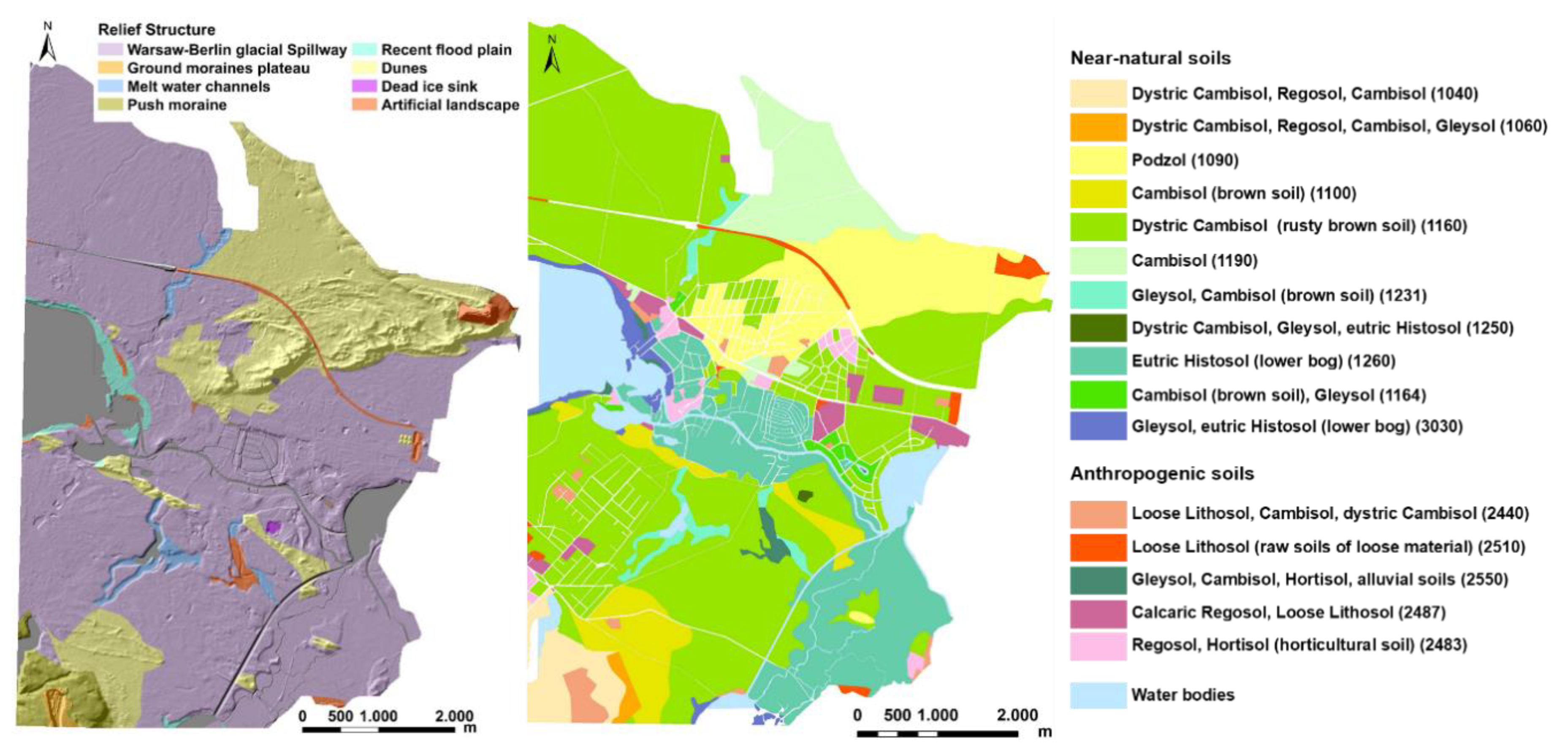
Figure 3.
Flow chart of the methodology followed for the landforms classification in the study area in ArcGIS and SAGA GIS.
Figure 3.
Flow chart of the methodology followed for the landforms classification in the study area in ArcGIS and SAGA GIS.

Figure 4.
Geomorphometric parameter derived from the LiDAR-DEM and related data for the study area. SLP is slope, PLANC is curvature surfaces or planar curvature, PROFC is profile curvature, GWD is ground water depth, HED is hydrography Euclidian distance, DISTWC is distance to nearest watercourse, FLOWA is flow accumulation, STI is sediment transport index, FM is fuzzy membership function, TWI is compound topographic index (SAGA wetness index), VDCNmod is modified vertical distance to channel network, CA is catchment area.

Figure 5.
Comparison of flow major channel networks derived from LiDAR-DEM, cell size of 1 m (left) and of resampled 5 m (right).
Figure 5.
Comparison of flow major channel networks derived from LiDAR-DEM, cell size of 1 m (left) and of resampled 5 m (right).

Figure 6.
Study area segmentation at different scale parameters; 5: too large (a), 20: too small (b), 10: good result (c). The background for the segmentation is the LiDAR-DEM with the resolution of 1 m.
Figure 6.
Study area segmentation at different scale parameters; 5: too large (a), 20: too small (b), 10: good result (c). The background for the segmentation is the LiDAR-DEM with the resolution of 1 m.
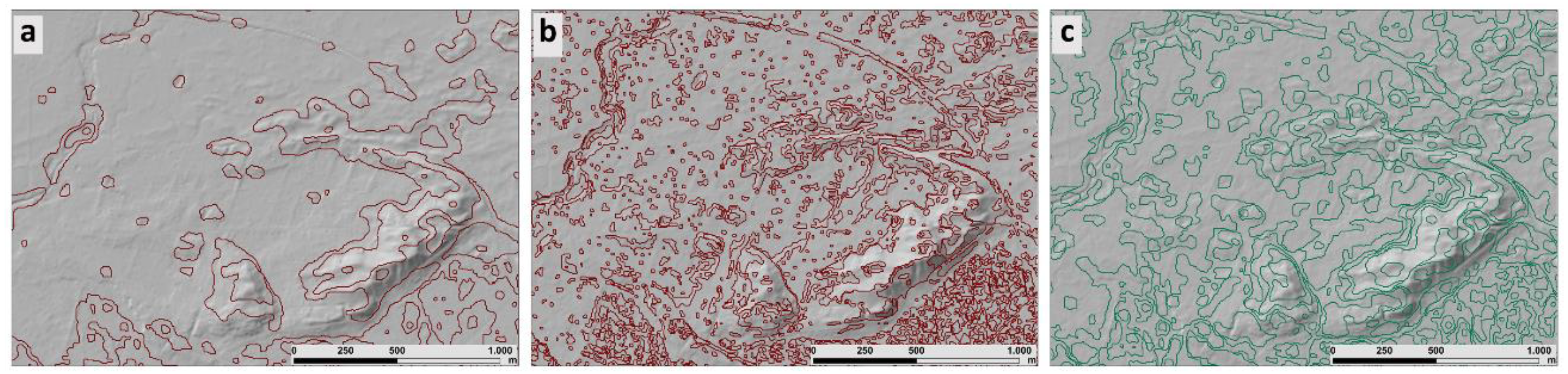
Figure 7.
Fuzzy membership functions to determine the slope classes based on the 0 to 1 linear scale adapted from [40] (left), and assigned fuzzy membership values for slope in the study area (right).
Figure 7.
Fuzzy membership functions to determine the slope classes based on the 0 to 1 linear scale adapted from [40] (left), and assigned fuzzy membership values for slope in the study area (right).

Figure 8.
Non-accumulated hypsometric curve of VDCNmod for areas classified as “flat land” based on the slope classification.
Figure 8.
Non-accumulated hypsometric curve of VDCNmod for areas classified as “flat land” based on the slope classification.

Figure 9.
Map of classification results based on a LiDAR-DEM (a) and an ASTER-DEM (b) for landforms in the city area.
Figure 9.
Map of classification results based on a LiDAR-DEM (a) and an ASTER-DEM (b) for landforms in the city area.

Figure 10.
Floodplain, terraced land and embankment: Landform classification based on LiDAR-DEM (a), landform classification based on ASTER-DEM (b) and orthophoto (0.2 m) (c).
Figure 10.
Floodplain, terraced land and embankment: Landform classification based on LiDAR-DEM (a), landform classification based on ASTER-DEM (b) and orthophoto (0.2 m) (c).

Figure 11.
Open and closed Depression: Landform classification based on LiDAR-DEM (a), landform classification based on ASTER-DEM (b) and orthophoto (0.2 m) (c).
Figure 11.
Open and closed Depression: Landform classification based on LiDAR-DEM (a), landform classification based on ASTER-DEM (b) and orthophoto (0.2 m) (c).
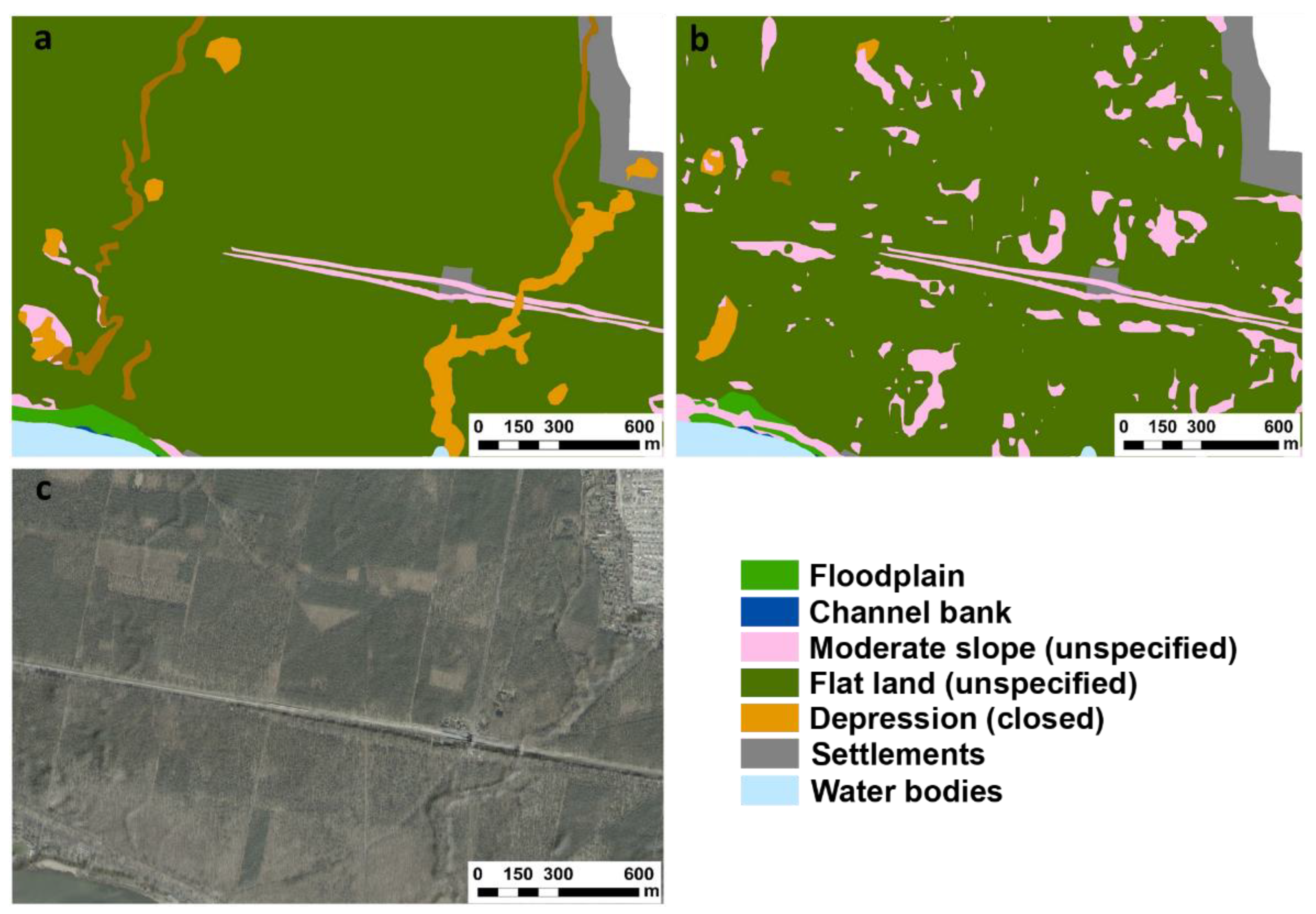

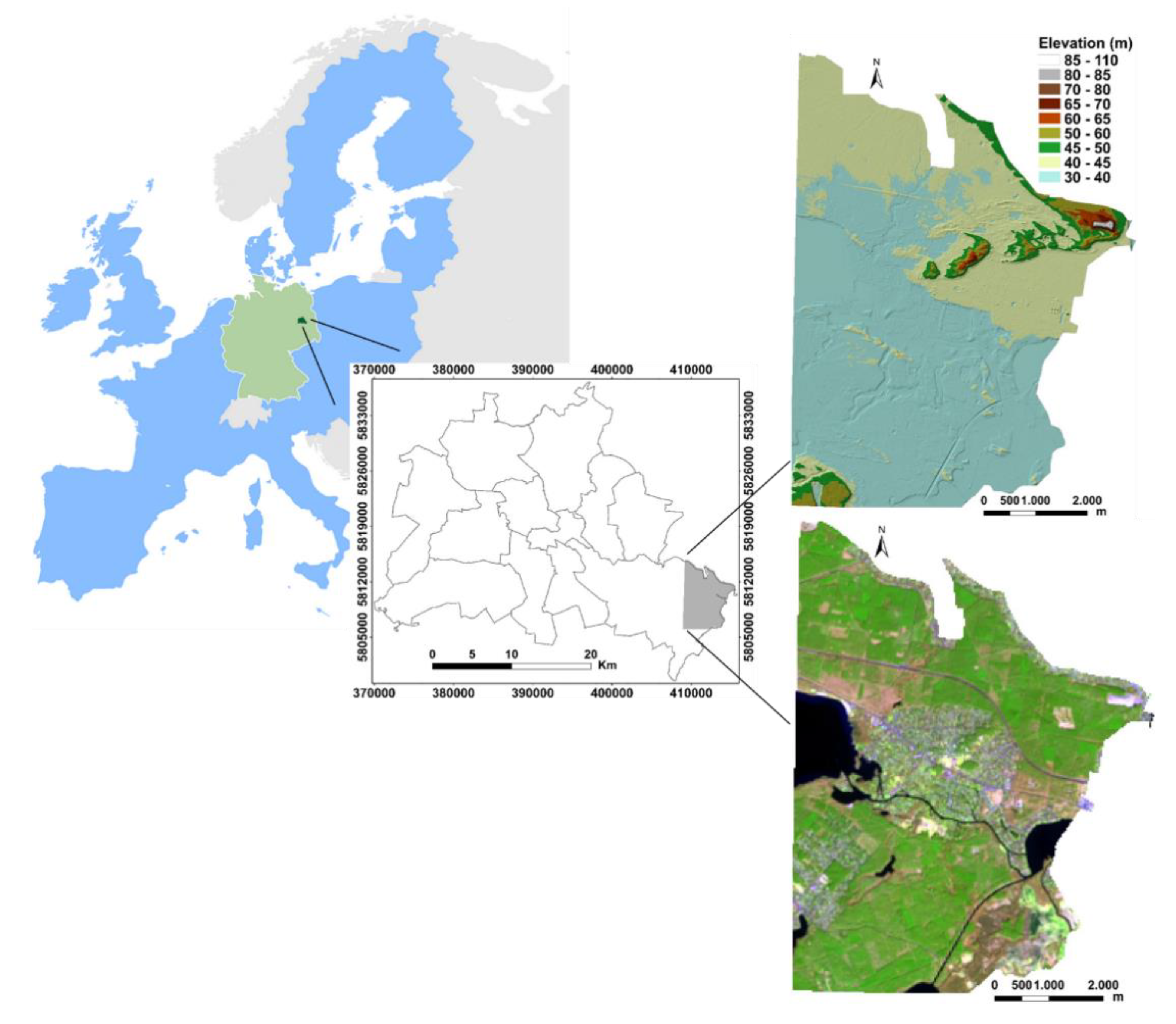
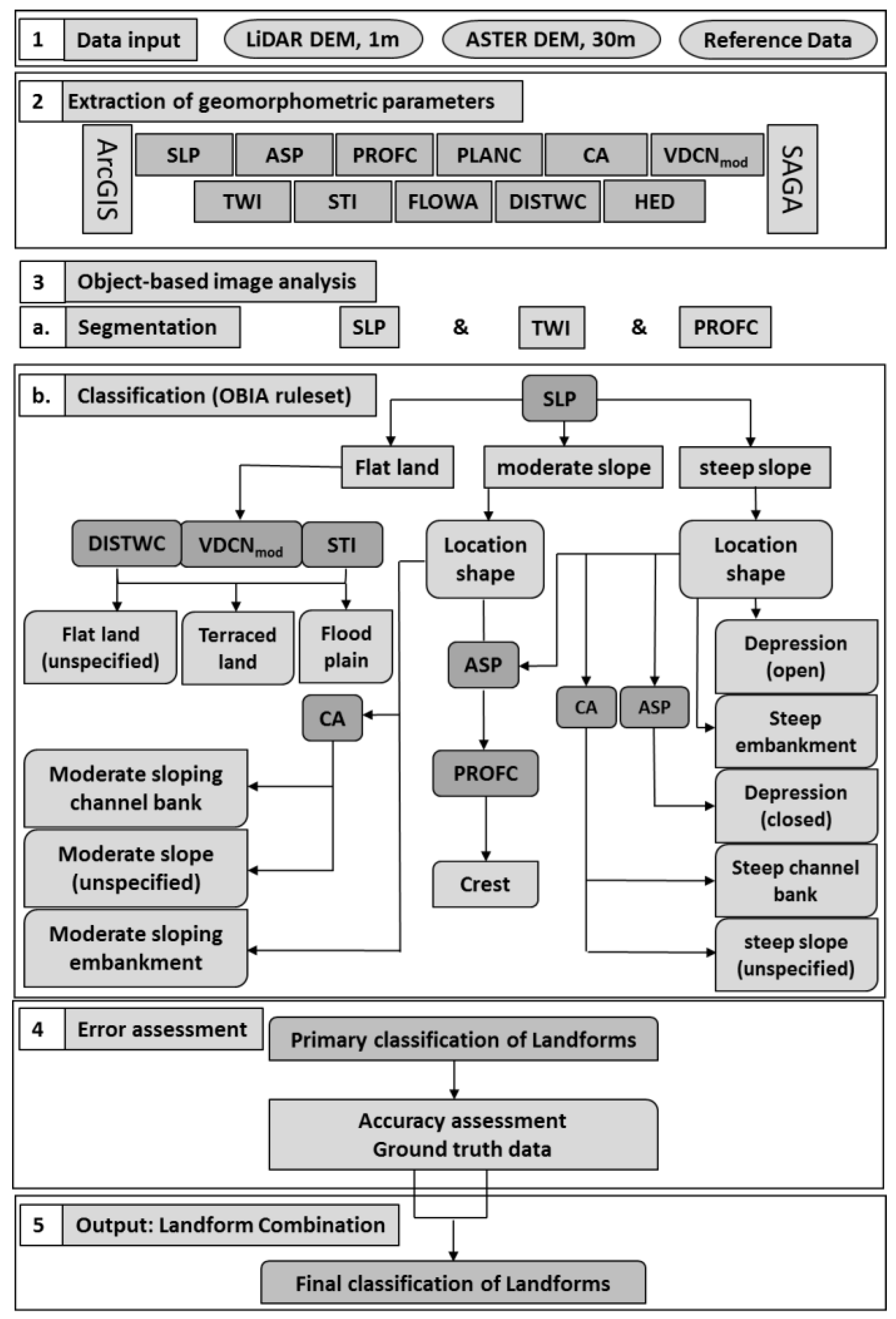
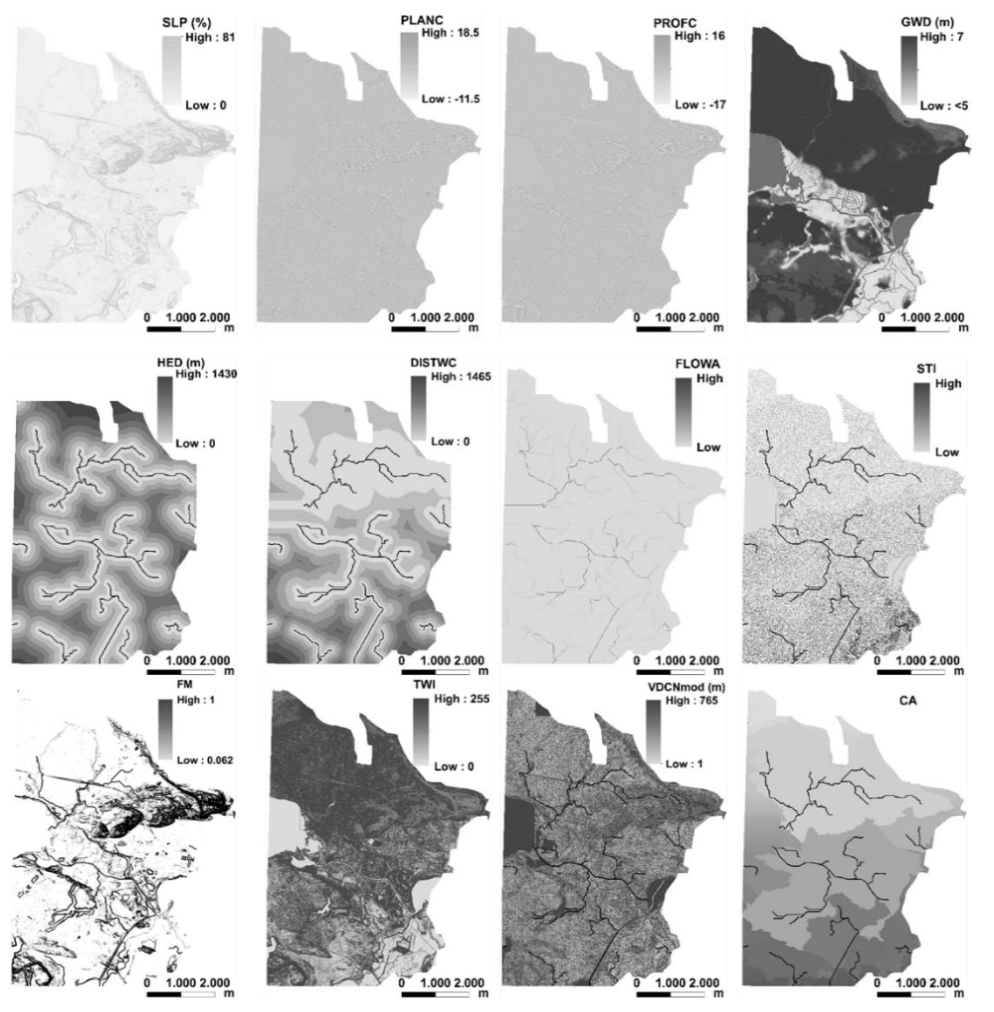
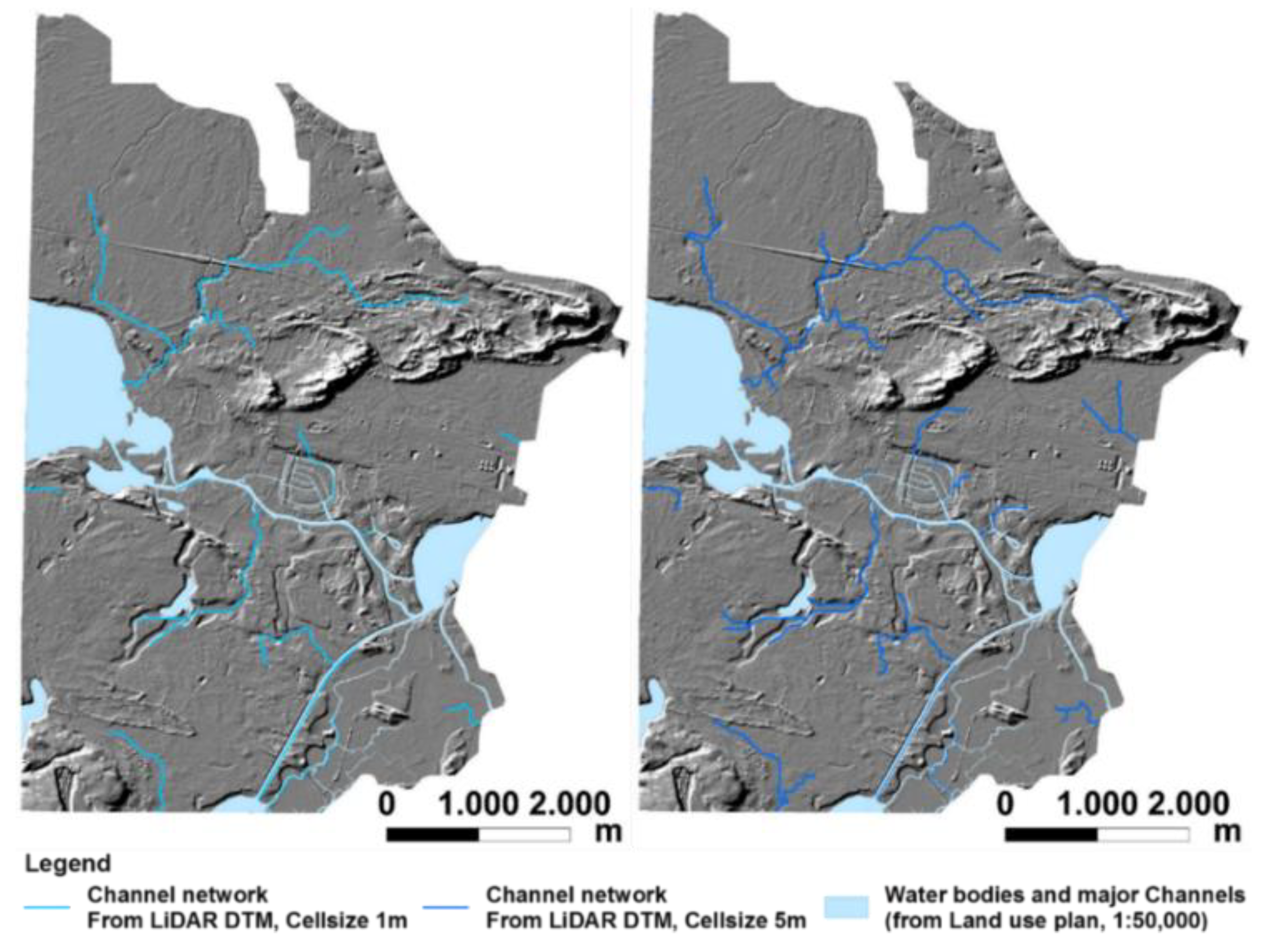
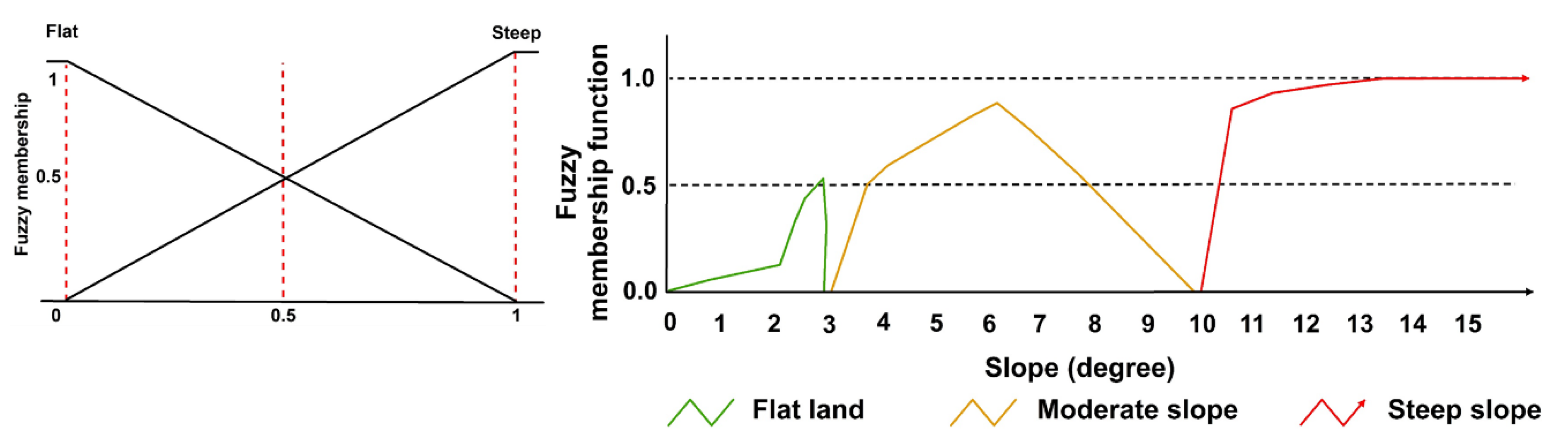
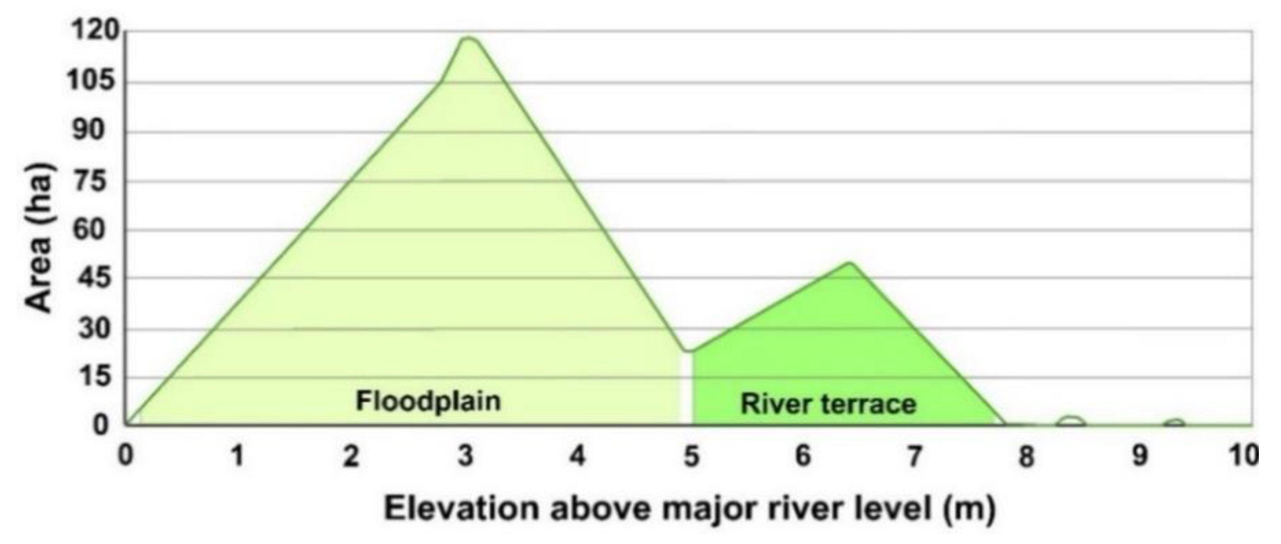
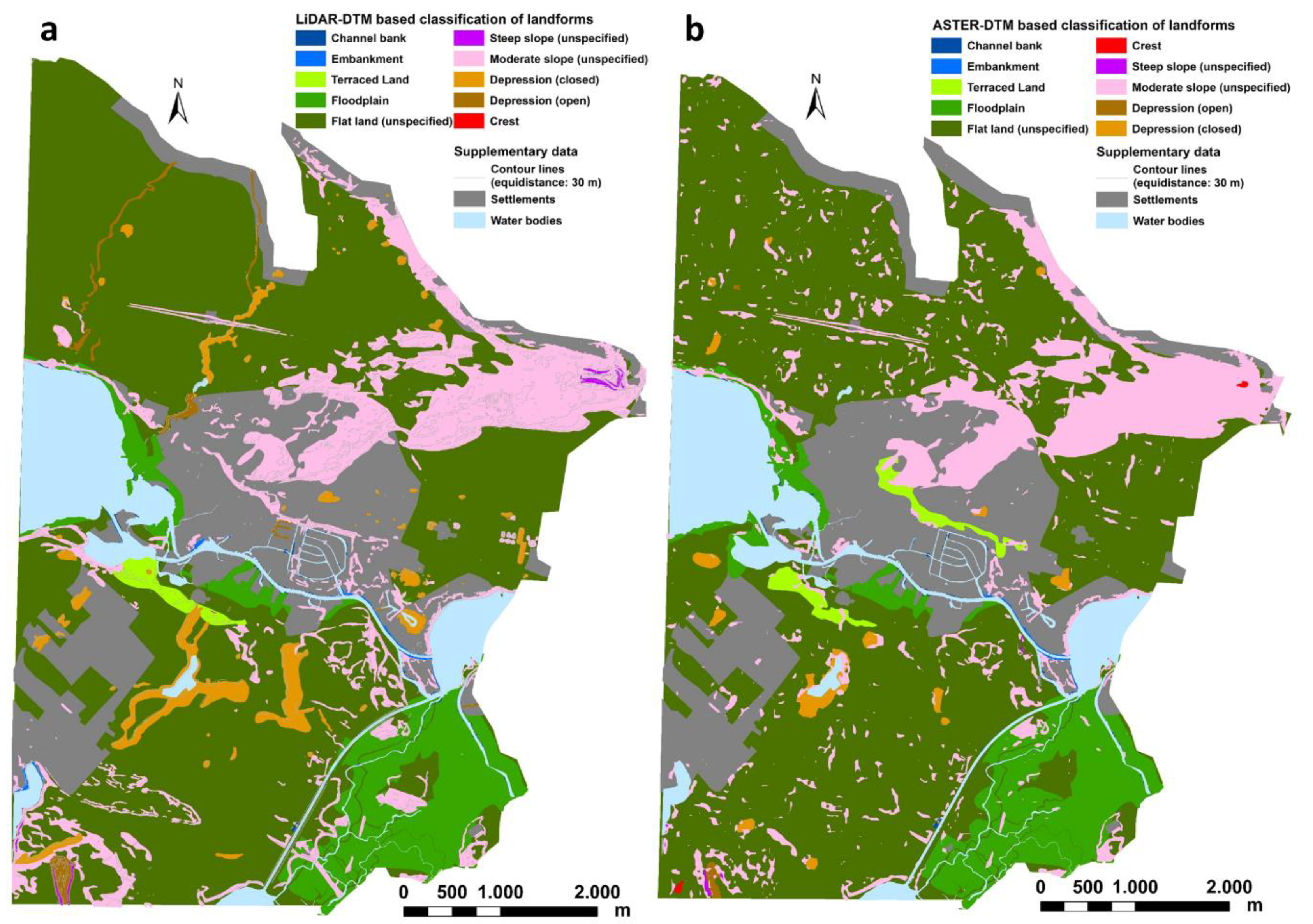
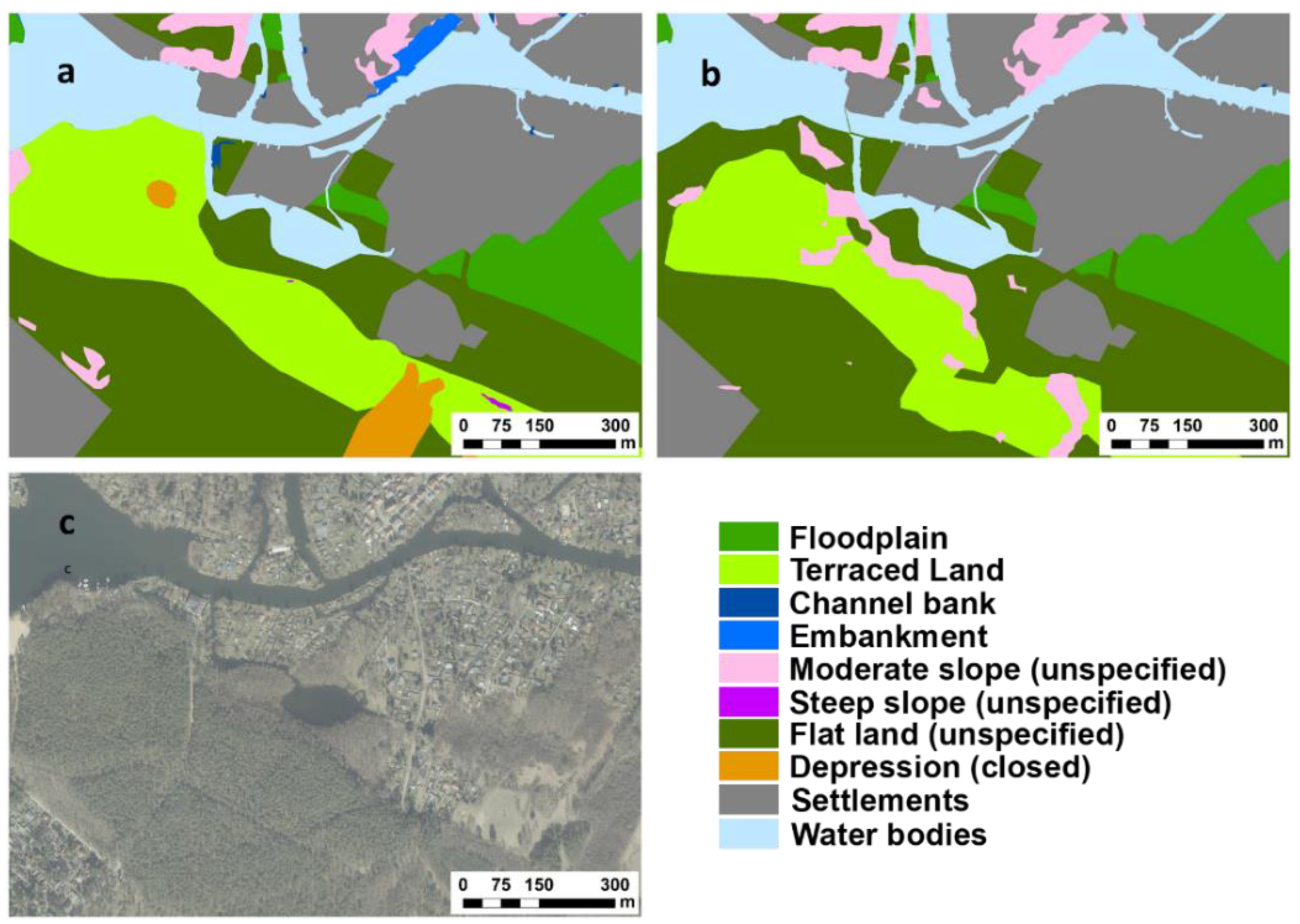
Table 1.
Relation of relief, substrate and soil types in the investigation area [57].
Table 1.
Relation of relief, substrate and soil types in the investigation area [57].
| Relief Structure | ID 1 | Predominant Soil Type | Typical Starting Substrate | (%) |
|---|---|---|---|---|
| Flood plain with alluvial dynamics (river flat) | 3030 | Gleysol, eutric Histosol (lower bog) | River sand | 2.06 |
| Ground moraines plateau | 2440 | Loose Lithosol (raw soils of loose material), Cambisol (brown soil), dystric Cambisol (rusty brown soils) | Loamy sand (glacial sands) | 0.81 |
| Sand dunes (dune landscape) | 1090 | Podzol | Fly-sand (wind-borne sand) on valley sand | 20.18 |
| 1100 1190 | Cambisol (brown soil) | |||
| 1060 | Dystric Cambisol (rusty brown soil), Regosol, Cambisol (colluvial brown soil), Gleysol | Loamy sand (glacial sands) | 0.75 | |
| Warsaw–Berlin glacial valley | 1160 | Dystric Cambisol (rusty brown soil) | Valley sand | 57.03 |
| 1164 | Cambisol (brown soil), Gleysol | |||
| 2487 | Calcaric Regosol, Loose Lithosol (raw soil of loose material) | |||
| 2483 | Regosol, Hortisol (horticultural soil) | |||
| 1260 | Eutric Histosol (lower bog) | Peat on valley sand | 12.23 | |
| Melt water channels | 1231 | Gleysol, Cambisol (brown soil) | Valley sand | 1.31 |
| Artificial structure (sand, industrial demolition, building rubble) | 2510 | Loose Lithosol (raw soils of loose material) | Rubble or accumulations of sand, industrial demolition, building rubble and backfilling | 2.25 |
| 2550 | Gleysol, Cambisol (brown soil), Hortisol (horticultural soil), alluvial soils | |||
| Push moraine/Landscape of sloping hill of loose material | 1040 | Dystric Cambisol (rusty brown soil), Regosol, Cambisol (brown soil) | Loamy sand (glacial sands), in places with embedded boulder loam (glacial loam) or marls | 2.76 |
| Dead ice sink/Small pond | 1250 | Dystric Cambisol (rusty brown soil), Gleysol, eutric Histosol (lower bog) | Valley sand, peat | 0.05 |
1 ID = The order of the soil associations and soil types in the concept map with a scale of 1:50,000 for the whole territory of Berlin, which is subdivided into near-natural soils and anthropogenic soils according to the degree of anthropogenic influence and the change of soils [57].
Table 2.
Geomorphometric parameters of the study area calculated from the LiDAR-DEM, ASTER-DEM and related data, which represent the input layers for a knowledge-based fuzzy landforms classification.
Table 2.
Geomorphometric parameters of the study area calculated from the LiDAR-DEM, ASTER-DEM and related data, which represent the input layers for a knowledge-based fuzzy landforms classification.
| Symbol | Geomorphometric Parameter | Software | Reference |
|---|---|---|---|
| LiDAR-DEM | Elevation | ArcGIS | [61] |
| ASTER-DEM | Elevation | ArcGIS | [62] |
| SLP | Slope | ArcGIS | [73] |
| ASP | Aspect | ArcGIS | [73] |
| PROFC | Profile curvature | ArcGIS | [74] |
| PLANC | Curvature surfaces or planar curvature | ArcGIS | [74] |
| CA | Catchment area | ArcGIS | [74] |
| VDCNmod | Modified vertical distance to channel network | SAGA-GIS | [6] |
| TWI | Compound topographic index (SAGA wetness index) | SAGA-GIS | [75] |
| STI | Sediment transport index | ArcGIS | [76,77] |
| GWD | Ground water depth | ArcGIS | [71] |
| FLOWA | Flow accumulation | ArcGIS | - |
| DISTWC | Distance to nearest watercourse | ArcGIS | - |
| HED | Hydrography Euclidian distance | ArcGIS | - |
| FM | Fuzzy membership function | ArcGIS | - |
Table 3.
Landforms in the study area with geomorphometric attributes.
| Landform | Relief Structure | Formation Process | Typical Starting Substrate | Properties |
|---|---|---|---|---|
| Crest | Dune | Aeolian, glacial | Fly-sand (wind-borne sand) | Low slope (1° < SLP < 3°), very low TWI |
| Hillside slope | Dunes, push moraine, ground moraines plateau, artificial landscape | Aeolian, glacial, human | Fly-sand (wind-borne sand), loamy sand (glacial sands), rubble or accumulations of sand, industrial demolition, building rubble and backfilling | Medium slope and high slope (SLP > 10°), very low TWI, high VDCN, specific CA, large std. dev. aspect |
| Flat land (unspecified) | Warsaw–Berlin glacial spillway | Glaciofluvial, fluvial | Valley sand, river sand | Low slope (SLP < 3°), medium TWI, low GWD |
| Depression (open, closed) | Dead ice sink, ground moraines plateau, melt water channels | Glacial, glaciofluvial | Valley sand, peat, loamy sand (glacial sands) | Low slope and medium slope (3° < SLP < 10°), high TWI, medium STI, medium and high GWD, low VDCN, low DISTWC |
| Embankment | Warsaw–Berlin glacial spillway, dune | Human | Sand, gravel, silt, clay | Medium slope and high slope (3 < SLP < 10°), medium TWI, medium GWD, close vicinity to fp ∩ tf U river |
| Terraced land | Warsaw–Berlin glacial spillway | Fluvial | Fluvial sediments (valley sand) | Medium slope (10° < SLP < 23°), very low TWI, high VDCN |
| Channel bank | Warsaw–Berlin glacial spillway | Fluvial | Fluvial sediments (valley sand) | Low slope and medium slope (1° < SLP < 10°), medium TWI, medium and high GWD, low DISTWC |
| Floodplain | Recent floodplain | Fluvial sediments (river sand with peat) | River sand with peat | Very low slope (SLP < 1°), very high TWI, medium STI, very high GWD, low VDCN, low DISTWC |
Table 4.
Description of landforms according to their morphological type (topographic position) according to Speight (2009) in the study area [83].
Table 4.
Description of landforms according to their morphological type (topographic position) according to Speight (2009) in the study area [83].
| Landform | Abbrev. | Description |
|---|---|---|
| Crest | cr | Landform element in the landscape that stands above all, or almost all, points in the adjacent terrain, with a positive plan and/or profile curvature |
| Moderate hillside slope | ms | Planar landform that is neither a crest nor a depression and has an inclination of 3–40%. |
| Steep hillside slope | ss | Planar landform that is neither a crest nor a depression and has an inclination >40% |
| Flat land (unspecified) | fl | Planar landform that is neither a crest nor a depression and is level or very gently inclined, with a slope < 3%. |
| Depression (open, closed) | de | Landform in the landscape that stands below all, or almost all, points in the adjacent terrain, with a negative plan and/or profile curvature, closed: local elevation minimum; open: extends at same or lower elevation |
| Embankment | eb | A bank (slope) is eroded and aggraded, and locally built up or excavated, by rarely active human agency, above the immediately surrounding land to redirect or prevent flooding by a river or lake, having an average slope > 1%. Embankments can be defined as narrow and elongated landforms that incline vertically towards the main slope direction, separating floodplains and river terraces or terraced land. |
| Terraced land | tl | Terraced land or terrace flats occur at stated heights above the top of the stream bank, including one or more terraces and often a flood plain. Relief is low < 35 m (elevation above major river level). |
| Channel bank | cb | Very short, very wide slope, moderately inclined to precipitous, forming the marginal upper parts of a stream channel and resulting from erosion or aggradation by channeled stream flow, resulting in changes of alignment, low < 35 m (elevation above major river level). |
| Floodplain | fp | Alluvial plain characterized by frequently active erosion and aggradation by channeled or overbank stream flow. Unless otherwise specified, ‘frequently active’ means that flow has an average recurrence interval of 50 years or less, having slope < 3%, low < 35 m (elevation above major river level). |
Table 5.
Confusion matrix for landform classification based on the LiDAR-DEM and reference data (sample points) set for whole study area. Where cr is crest, ms is moderate hillside slope, ss is steep hillside slope, fl is flat land (unspecified), de is depression (open, closed), eb is embankment, tl is terraced land, cb is channel bank and fb is floodplain.
| Sample Points | Classification Based on Reference Data | |||||||||||
|---|---|---|---|---|---|---|---|---|---|---|---|---|
| Classification based on LiDAR-DEM | cr | ss | ms | fl | de | eb | tl | cb | fb | Total | UA (%) | |
| cr | 10 | 1 | 3 | 0 | 0 | 0 | 0 | 0 | 0 | 14 | 71.42 | |
| ss | 0 | 44 | 29 | 1 | 0 | 0 | 0 | 0 | 0 | 74 | 59.46 | |
| ms | 0 | 0 | 7639 | 620 | 0 | 46 | 91 | 21 | 0 | 8417 | 90.75 | |
| fl | 0 | 0 | 592 | 10,349 | 27 | 0 | 0 | 0 | 0 | 10,968 | 94.35 | |
| de | 0 | 0 | 0 | 0 | 78 | 0 | 0 | 0 | 0 | 78 | 100.00 | |
| eb | 0 | 0 | 0 | 0 | 0 | 54 | 0 | 3 | 0 | 57 | 94.73 | |
| tl | 0 | 0 | 12 | 8 | 0 | 0 | 71 | 0 | 5 | 96 | 73.95 | |
| cb | 0 | 0 | 6 | 0 | 0 | 0 | 0 | 147 | 0 | 153 | 96.07 | |
| fb | 0 | 0 | 0 | 4 | 0 | 0 | 0 | 0 | 79 | 83 | 95.18 | |
| Total | 10 | 45 | 8281 | 10,982 | 105 | 100 | 162 | 171 | 84 | 19,940 | ||
| PA (%) | 100 | 97.77 | 92.24 | 94.20 | 74.28 | 54.00 | 43.83 | 85.96 | 94.00 | |||
| Overall accuracy = 92.63% and kappa = 85.87%. | ||||||||||||
Table 6.
Correlation of landforms classification results based on the LiDAR-DEM and soil types according to the digital soil map 1:50,000 for study area [57].
Table 6.
Correlation of landforms classification results based on the LiDAR-DEM and soil types according to the digital soil map 1:50,000 for study area [57].
| Soil Type | Landform | ||||||||||
|---|---|---|---|---|---|---|---|---|---|---|---|
| ID 1 | cr | ss | ms | fl | de | eb | tl | cb | fb | ||
| Soils of mainly natural litho- and pedo-genesis | Dystric Cambisol (rusty brown soil), Regosol, Cambisol (brown soil) | 1040 | 0.00% | 0.00% | 4.32% | 0.00% | 0.00% | 8.77% | 0.00% | 3.23% | 0.00% |
| Dystric Cambisol (rusty brown soil), Regosol, Cambisol (colluvial brown soil), Gleysol | 1060 | 0.00% | 0.00% | 0.57% | 0.92% | 0.00% | 0.00% | 0.00% | 0.00% | 0.00% | |
| Podzol, Cambisol (brown soil) | 1090 1100 1190 | 0.00% | 44.59% | 38.51% | 0.50% | 3.85% | 0.00% | 94.00% | 3.27% | 0.00% | |
| Dystric Cambisol (rusty brown soil), Cambisol (brown soil), Gleysol | 1160 1164 | 0.00% | 0.00% | 28.82% | 67.02% | 38.46% | 64.92% | 6.00% | 13.73% | 0.00% | |
| Cambisol (brown soil), Gleysol | 1231 | 0.00% | 0.00% | 4.65% | 0.00% | 29.49% | 22.81% | 0.00% | 3.92% | 0.00% | |
| Dystric Cambisol (rusty brown soil), Gleysol, eutric Histosol (lower bog) | 1250 | 0.00% | 0.00% | 0.00% | 0.00% | 3.85% | 0.00% | 0.00% | 0.00% | 0.00% | |
| Eutric Histosol (lower bog) | 1260 | 0.00% | 0.00% | 12.44% | 7.66% | 3.84% | 1.75% | 0.00% | 71.90% | 88.31% | |
| Gleysol, eutric Histosol (lower bog) | 3030 | 0.00% | 0.00% | 0.00% | 17.01% | 0.00% | 0.00% | 0.00% | 3.92% | 11.69% | |
| Soils of anthropogenic litho- and pedogenesis | Loose Lithosol (raw soils of loose material), Gleysol | 2430 | 0.00% | 10.81% | 0.00% | 0.00% | 0.00% | 0.00% | 0.00% | 0.00% | 0.00% |
| Loose Lithosol (raw soils of loose material), Cambisol (brown soil), dystric Cambisol (rusty brown soils) | 2440 | 0.00% | 4.41% | 3.77% | 0.00% | 11.54% | 0.00% | 0.00% | 0.00% | 0.00% | |
| Hortisol (horticultural soil) | 2483 | 0.00% | 0.00% | 0.00% | 0.00% | 2.56% | 1.75% | 0.00% | 0.00% | 0.00% | |
| Calcaric Regosol, loose Lithosol (raw soil of loose material), Regosol | 2487 | 0.00% | 18.92% | 4.98% | 0.00% | 0.00% | 0.00% | 0.00% | 0.00% | 0.00% | |
| Loose Lithosol (raw soils of loose material) | 2510 | 100% | 20.27% | 1.94% | 0.00% | 0.00% | 0.00% | 0.00% | 0.00% | 0.00% | |
| Gleysol, Cambisol (brown soil), Hortisol (horticultural soil), alluvial soils | 2550 | 0.00% | 0.00% | 0.00% | 0.00% | 6.41% | 0.00% | 0.00% | 0.00% | 0.00% | |
1 ID = The order of the soil associations and soil types in the concept map with a scale of 1: 50,000 for the whole territory of Berlin, which is subdivided into near-natural soils and anthropogenic soils according to the degree of anthropogenic influence and the change of soils. Where cr is crest, ms is moderate hillside slope, ss is steep hillside slope, fl is flat land (unspecified), de is depression (open, closed), eb is embankment, tl is terraced land, cb is channel bank and fb is floodplain [57].
Table 7.
Confusion matrix for landform classification based on the ASTER-DEM and reference data (sample points) set for whole study area. Where cr is crest, ms is moderate hillside slope, ss is steep hillside slope, fl is flat land (unspecified), de is depression (open, closed), eb is embankment, tl is terraced land, cb is channel bank and fb is floodplain.
| Sample Points | Classification Based on Reference Data | |||||||||||
|---|---|---|---|---|---|---|---|---|---|---|---|---|
| Classification based on ASTER-DEM | cr | ss | ms | fl | de | eb | tl | cb | fb | Total | UA (%) | |
| cr | 4 | 0 | 0 | 0 | 0 | 0 | 0 | 0 | 0 | 4 | 100.00 | |
| ss | 0 | 22 | 0 | 0 | 0 | 0 | 0 | 0 | 0 | 22 | 100.00 | |
| ms | 6 | 46 | 3876 | 817 | 0 | 58 | 59 | 31 | 0 | 4893 | 79.21 | |
| fl | 0 | 0 | 4405 | 9143 | 334 | 0 | 4 | 0 | 0 | 13,886 | 65.84 | |
| de | 0 | 0 | 0 | 138 | 92 | 0 | 0 | 0 | 0 | 230 | 40.00 | |
| eb | 0 | 0 | 0 | 0 | 0 | 32 | 00 | 4 | 0 | 36 | 88.88 | |
| tl | 0 | 0 | 0 | 37 | 0 | 0 | 92 | 0 | 55 | 184 | 50.00 | |
| cb | 0 | 0 | 0 | 0 | 0 | 0 | 0 | 16 | 0 | 16 | 100.00 | |
| fb | 0 | 0 | 0 | 85 | 2 | 0 | 0 | 0 | 582 | 669 | 86.99 | |
| Total | 10 | 68 | 8281 | 10,220 | 428 | 90 | 155 | 51 | 637 | 19,940 | ||
| PA (%) | 40.00 | 32.35 | 46.80 | 89.46 | 21.49 | 35.35 | 38.06 | 31.37 | 91.36 | |||
| Overall accuracy = 69.50% and kappa = 43.59%. | ||||||||||||
Table 8.
Correlation of LiDAR-DEM based and ASTER-DEM based classifications and share of each category from the total area. Where cr is crest, ms is moderate hillside slope, ss is steep hillside slope, fl is flat land (unspecified), de is depression (open, closed), eb is embankment, tl is terraced land, cb is channel bank and fb is floodplain.
| Category | Classification Based on LiDAR-DEM | Classification Based on ASTER-DEM | ||||||
|---|---|---|---|---|---|---|---|---|
| Sample Points | Total of Sample Points | Correlation | Area (%) | Sample points | Total of Sample Points | Correlation | Area (%) | |
| cr | 10 | 14 | 71.20% | 0.02 | 4 | 4 | 70.10% | 0.03 |
| ss | 44 | 74 | 59.40% | 0.21 | 22 | 22 | 59.10% | 0.04 |
| ms | 7639 | 8417 | 90.6% | 8.53 | 3876 | 4893 | 73.00% | 8.65 |
| fl | 10,349 | 10,968 | 94.20% | 70.23 | 9143 | 13,886 | 75.50% | 71.01 |
| de | 78 | 78 | 98.30% | 5.28 | 92 | 230 | 40.00% | 1.72 |
| eb | 54 | 57 | 83.50% | 0.29 | 32 | 36 | 28.30% | 0.15 |
| tl | 71 | 96 | 58.50% | 0.83 | 92 | 184 | 34.30% | 1.45 |
| cb | 147 | 153 | 73.00% | 0.17 | 16 | 16 | 17.02% | 0.10 |
| fb | 79 | 83 | 95.30% | 14.44 | 582 | 669 | 86.90% | 16.85 |
| Total | 18,471 | 19,940 | 82.10% | 100 | 13,859 | 19,940 | 55.65% | |
| Overall correlation = 68.88% | ||||||||
© 2020 by the author. Licensee MDPI, Basel, Switzerland. This article is an open access article distributed under the terms and conditions of the Creative Commons Attribution (CC BY) license (http://creativecommons.org/licenses/by/4.0/).
Share and Cite
MDPI and ACS Style
Mohamed, M.A. Classification of Landforms for Digital Soil Mapping in Urban Areas Using LiDAR Data Derived Terrain Attributes: A Case Study from Berlin, Germany. Land 2020, 9, 319. https://doi.org/10.3390/land9090319
AMA Style
Mohamed MA. Classification of Landforms for Digital Soil Mapping in Urban Areas Using LiDAR Data Derived Terrain Attributes: A Case Study from Berlin, Germany. Land. 2020; 9(9):319. https://doi.org/10.3390/land9090319
Chicago/Turabian StyleMohamed, Mohamed Ali. 2020. "Classification of Landforms for Digital Soil Mapping in Urban Areas Using LiDAR Data Derived Terrain Attributes: A Case Study from Berlin, Germany" Land 9, no. 9: 319. https://doi.org/10.3390/land9090319
Note that from the first issue of 2016, this journal uses article numbers instead of page numbers. See further details here.