Article

Supporting Adaptive Connectivity in Dynamic Landscapes

by
Megan K. Jennings
1,2,*,
Katherine A. Zeller
3 and
Rebecca L. Lewison
1,2
1
Biology Department, San Diego State University, 5500 Campanile Drive, San Diego, CA 92182-4614, USA
2
Institute for Ecological Monitoring and Management, San Diego State University, San Diego, CA 92182-4614, USA
3
Aldo Leopold Wilderness Research Institute, Rocky Mountain Research Station, USDA Forest Service, Missoula, MT 59801, USA
*
Author to whom correspondence should be addressed.
Land 2020, 9(9), 295; https://doi.org/10.3390/land9090295
Submission received: 28 July 2020 / Revised: 23 August 2020 / Accepted: 25 August 2020 / Published: 26 August 2020
(This article belongs to the Special Issue Dynamic Landscape Connectivity)

Abstract

:
A central tenet of landscape conservation planning is that natural communities can be supported by a connected landscape network that supports many species and habitat types. However, as the planning environment, ecological conditions, and risks and stressors change over time, the areas needed to support landscape connectivity may also shift. We demonstrate an approach designed to assess functional and structural connectivity of an established protected area network that has experienced landscape and planning changes over time. Here we present an approach designed to inform adaptive planning for connectivity with a complementary suite of analytical techniques. Using existing occurrence, movement, and genetic data for six focal species, we create a spatially explicit connectivity assessment based on landscape resistance, paired with a landscape feature geodiversity analysis. Although factors such as cost, conservation goals, and land management strategies must be taken into account, this approach provides a template for leveraging available empirical data and robust analyses to evaluate and adapt planning for protected area networks that can preserve and promote both functional and structural connectivity in dynamic landscapes.

1. Introduction

A central tenet of large-scale conservation planning is that viable populations and natural communities can be supported by a connected protected area network (also referred to as an ecological network) across the landscape [1,2]. Landscape connectivity allows for movement among patches of suitable habitat [3], reduces the chance of extinction and the effects of environmental variability on small populations [4], and maintains gene flow in patchy landscapes [5]. Despite the recognized ecological importance, incorporating connectivity into landscape conservation strategies is arguably one of the most challenging steps in conservation planning and reserve design [2,6], particularly as the planning environment, ecological conditions, stressors, and risks change over time.
One challenge in protecting connectivity across ecological networks is addressing the ability of the network to adapt to changes over time in conservation plans. This is particularly relevant for networks created in 1990s, the early years of landscape-scale planning efforts, when protected area networks could not benefit from advanced connectivity approaches that have since been developed and widely adopted. However, even in more recently developed networks, maintaining connectivity over time presents a persistent challenge. Many landscape-scale conservation plans and protected area networks are designed and implemented over multiple years or even decades, intended to guide conservation and management actions for preserving biodiversity over long time periods. However, few networks consider the dynamics in ecological, conservation, and planning conditions that can occur over these time frames. Changes in ecological conditions, such as land-use, the extent of fragmentation, habitat quality, and the conservation status of the populations established networks were intended to protect can all have profound impacts on landscape connectivity [2]. Incorporating these ecological or landscape changes may be particularly important to maintain connectivity across the landscape matrix, the substantial portion of the landscape that extends beyond designated core areas, where changes are most likely to arise [7,8]. In addition to these ecological dynamics, connectivity will be impacted by changes in institutional and planning dimensions [9] as plans, regulations and policies are also likely to change over time [10]. Although planners and resource managers recognize that ecological and institutional conditions will change, relatively little attention has been given to develop adaptive approaches to maintain and improve connectivity over long-term planning and implementation efforts.
The importance of maintaining and improving landscape connectivity in protected area networks was identified by the Convention on Biological Diversity as an Aichi Biodiversity Target for 2020 [11], but recent evaluations have found that it is unlikely this goal can be met without additional focus and concerted action [12]. To enhance the likelihood of success in meeting connectivity targets, connectivity efforts will need to include analytical and planning approaches that allow for an iterative process to accommodate and adapt to ecological and institutional change. Adaptive strategies to address dynamic conditions are commonly used in natural resource and land management and have been explored in conservation planning more generally [13,14,15], but connectivity planning and implementation is not often approached from this adaptive perspective. Yet, integrating dynamic conditions into connectivity planning is critical, especially in ex-urban or urbanizing regions where active development and habitat fragmentation threaten functionality [16]. Specifically, there is a need for assessment techniques to evaluate and adapt protected area network plans to address changes in ecological and planning contexts to ensure connectivity goals remain current, relevant, and feasible.
Assessments often evaluate connectivity either from a structural or functional perspective. Structural connectivity, which was more commonly applied in early protected area network planning, considers the physical connections among patches of habitat, whereas functional connectivity accounts for how organisms respond to the physical and biological conditions of the landscape. However, quantifying or assessing functional landscape connectivity under dynamic conditions presents a particular challenge given its context-dependent nature [2] and the expense and effort of acquiring data for species of interest [17]. Fortunately, analytical approaches to measure and quantify connectivity with a variety of data sources have expanded in recent years and can be applied even when detailed movement data are not available and information on dispersal and movement is limited. In the last decade, a range of empirical data types, extents, and resolutions [18] have been used to validate connectivity models and assessments [19,20,21,22]. However, these methods have not been widely used to inform the design of protected area networks or evaluate how well those networks are meeting connectivity goals over time given changes in the planning environment or ecological conditions.
Functional connectivity assessments often rely on a focal species approach to identify land parcels that will support movement and metapopulation persistence [23,24]. A multi-species framework can be advantageous, especially in landscapes where initial conservation planning efforts pre-date many of the analytical advances in connectivity modeling [25,26,27]. In addition, pairing species-focused analyses with structural landscape approaches can serve to connect structural connectivity as well the features of the landscape that facilitate movement for a wide range of species as conditions and priorities shift [28,29]. Species-agnostic approaches that have been developed to structurally connect large natural areas in response to environmental changes in the landscape, such as land facet analyses which focus on geological, topographic, and climatic diversity, can support these efforts [30,31,32].
We developed a multi-species connectivity assessment paired with land facet analysis to evaluate connectivity in a long-established protected area network, the San Diego Multiple Species Conservation Plan (MSCP). Using this network, we demonstrate a flexible and scalable approach to evaluate connectivity across a protected area network that can be used to adapt conservation plans in response to ongoing or projected dynamics in planning, land-use, and habitat conditions. The analysis, which relies on existing empirical data, capitalizes on and leverages considerable investments that have been made in species-level surveys, monitoring programs, and species-focused research. We use a range of data types to consider local-scale movements within home ranges, gene flow, short range dispersal events for dispersal-limited species, as well as longer-range movements such as dispersal of wide-ranging species. As such, this approach can be used to evaluate whether protected area networks at any stage of planning or implementation are meeting connectivity goals over time as conditions change, allowing for adaptive management and planning to retrofit the existing network to support and promote connectivity. Our findings illustrate the repeatability and utility of an empirical, multi-species approach complemented with a land facet analysis to assess connectivity in a dynamic planning environment that can readily be adapted to different regions, scenarios, species, and habitats.

2. Materials and Methods
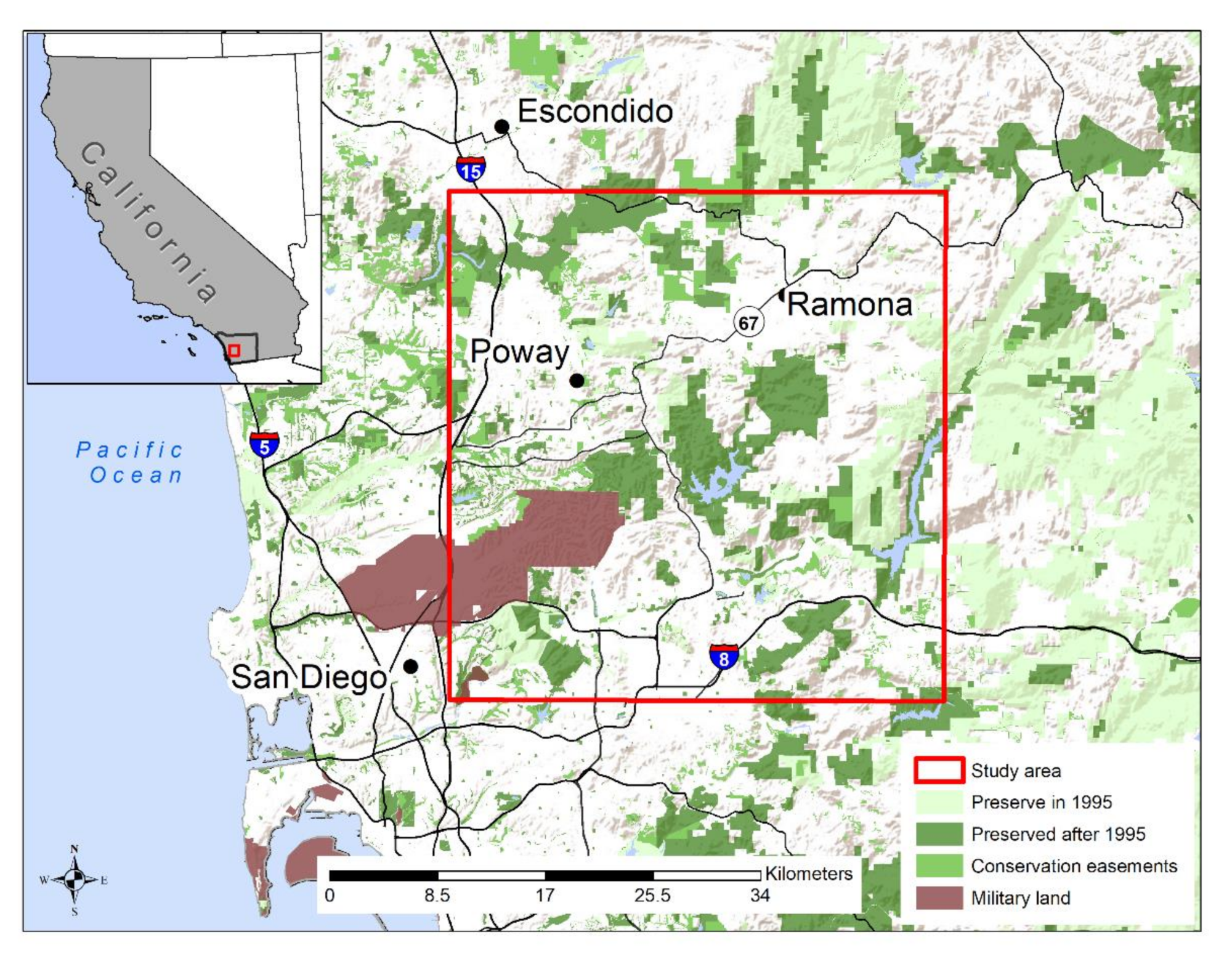
2.1. Study Area

In San Diego County, growth and development pressure are concentrated in the western third of the county along the coast (Figure 1). To address the associated habitat loss and declining populations of rare species, a conservation plan was developed in the 1990s within San Diego County, the San Diego MSCP (Additional details in Appendix A1; [33]). This plan was focused on assembling a network of conserved land that would ensure protection of important habitats and species and streamline environmental review for proposed developments in pre-approved areas. In the two decades since implementation began, the preserve network has nearly doubled. However, functional connectivity was not explicitly incorporated into planning efforts. Although regional [34,35] and statewide efforts [36] that were undertaken to address connectivity provided some information for this region, connectivity has not been thoroughly evaluated at the sub-regional or plan level since implementation of the conservation plan first began in 1996. Meanwhile, continued development threatens the functioning of this plan area as a true network.
This study focused on lands surrounding a rural highway, State Route (SR) 67, that bisects a portion of the existing preserve network where there are multiple preserves on either side of the highway. The natural habitats and conserved lands in the area are primarily publicly owned and include a number of lands owned and managed by State, County, and City governments as well as National Forest in the eastern portion of the study area. The primary analysis area encompassed ~540 km2. Here, we use the term “conserved lands” to describe areas within the network considered to be protected from conversion to urban and suburban development, but may be subject to utility infrastructure development, recreational activities, or extractive uses.
Elevation across the study site ranged from 58 m in the western section of the San Diego River to 1110 m at the highest point of the study area, El Cajon Mountain. Vegetation types varied with elevation, distance to the coast, and proximity to the roadway, but the study area was predominantly a shrubland ecosystem. Vegetation associations across these areas included coastal sage scrub, chaparral, oak woodland, grasslands, riparian zones, as well as urban and altered areas. Within the highway right-of-way and near industrial and urbanized areas, vegetation was dominated by a mix of non-native plants and barren areas, interspersed with coastal sage scrub and chaparral. The Mediterranean climate of the study region is characterized by hot, dry summers and mild, wet winters with precipitation often less than 300 mm.

2.2. Focal Species and Environmental Variables

We selected six focal species with adequate data, both in terms of quantity and spatial distribution, for analysis to represent a range of movement abilities, habitat associations, and sensitivities to relevant stressors. Data sources for the focal species—puma (Puma concolor), bobcat (Lynx rufus), southern mule deer (Odocoileus hemionus fuliginatus), wrentit (Chamaea fasciata), big-eared woodrat (Neotoma macrotis), and California mouse (Peromyscus californicus)—are listed in Table 1. We selected the bobcat and puma to represent wide-ranging habitat generalists and capture movement among core areas of the network for both moderate distances (i.e., bobcat) and much larger distances (i.e., puma), with pumas demonstrating high sensitivity to areas of human development and activity and bobcats demonstrating moderate sensitivity [37]. We included the southern mule deer, which is a nonmigratory subspecies with limited home range and dispersal movements [38], as they are a regional species of conservation concern thought to be affected by roadways and dense urbanization. The wrentit, big-eared woodrat, and California mouse are all shrubland associates that require intact chaparral or coastal sage scrub habitats and have more restricted movements [39]. The wrentit is a strict scrub and chaparral associate that is sensitive to the continuity of vegetative cover because its flight is limited to short and low bursts, making it susceptible to population-level effects of wildfires [40], habitat degradation, and fragmentation by roads [41], such as the highway that bisects our study area. Big-eared woodrats occur in shrubland, riparian, and woodland habitats and were included as a focal species to represent local movements among these different habitat types. Finally, we selected the California mouse to incorporate local movements through areas of dense shrub canopy cover on steep, mesic slopes, which are heterogeneously distributed across our study area. Although we originally evaluated several herpetofauna species to include in our connectivity analyses, we were relying on existing models for these species that were ultimately not suitable for modeling connectivity as there was a scale mismatch between the existing models and our scale of interest.
We identified environmental variables thought to affect habitat use and movement for each focal species. These included topographic, land cover, water, and human development variables (Additional details in Supplementary Materials S1, Table S1). To assemble multiscale models that would allow us to consider how our selected species perceive environmental variables in the landscape, we used an ecological neighborhood approach [49,50]. We applied a Gaussian smooth to each variable at a variety of biologically relevant spatial scales for each species based on movement and home range information we gathered for each species from a combination of published literature, movement data, and expert opinion. We used an information-theoretic approach to select the most appropriate scale for each variable (see Supplementary Materials S1 for more details). We tested scales ranging from 30 m to 180 m for California mouse and woodrat, 30 m to 360 m for wrentit, 30 m to 2160 m for mule deer, 30 m to 2000 m for bobcat, and 30 m to 10,000 m for puma.

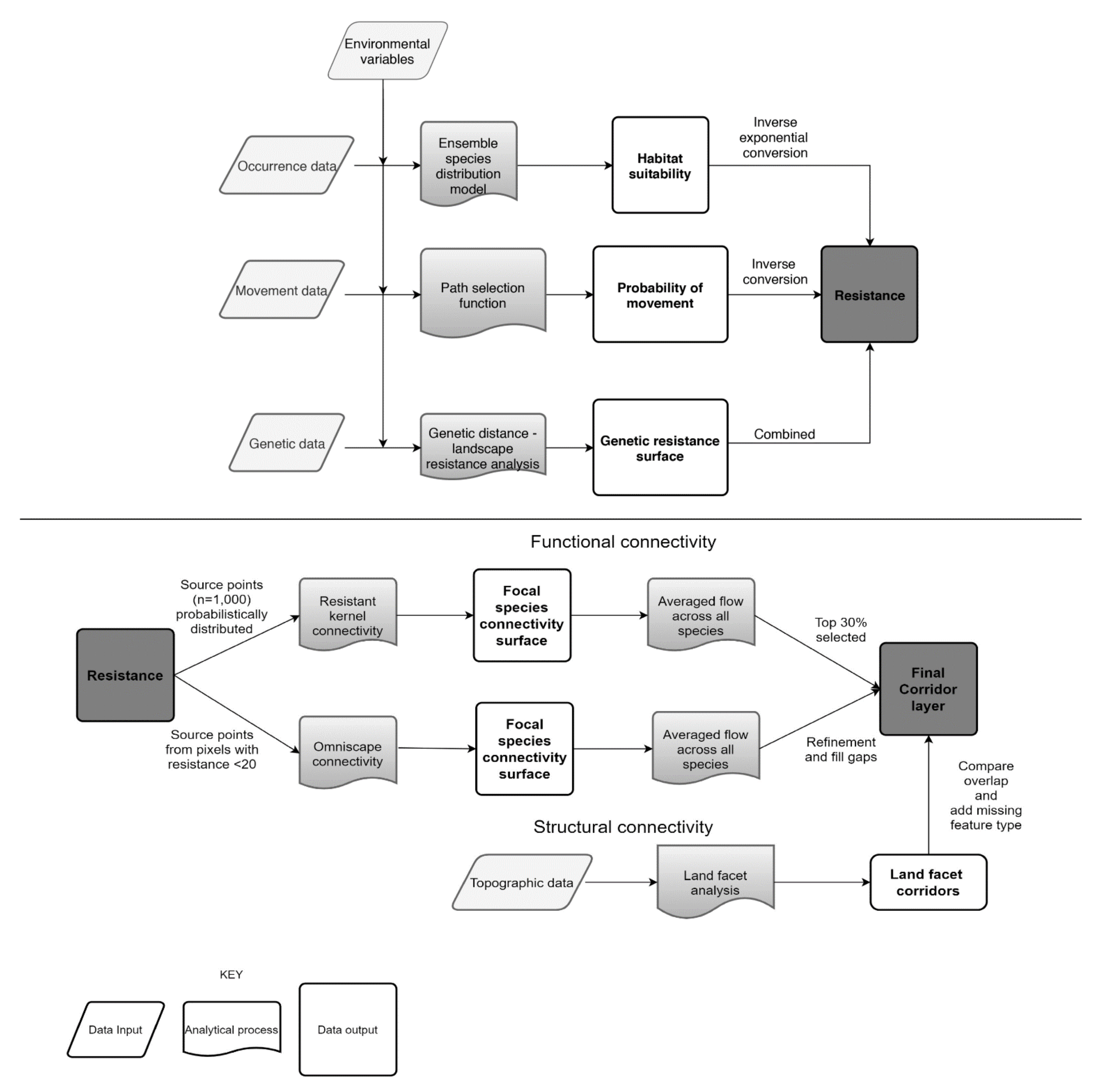
2.3. Modeling Approach Overview

We identified a suite of analytical techniques that would support comprehensive, data-driven analyses to assess and map connectivity, employing a resistance-based approach [51] to model flow across the landscape. To generate informative resistance surfaces, we conducted movement, habitat, and genetic analyses that were most appropriate for the types of data that were available for each species (Table 1). Multi-species landscape-level corridors were derived by: (1) identifying available data sources and selected species reviewed by local experts and data sharers; (2) running spatially explicit models at a 30-m resolution to estimate movement, habitat use, and resistance to movement at the county level for each species; (3) modeling landscape linkages for each species and a complementary land facet corridor; and (4) combining results across species and land facets to create a multi-species linkage map. Methodological approaches are summarized below with additional details in Supplementary Materials S1–S4 and [21].

2.4. Habitat Use, Movement, and Resistance Modeling

To develop high-quality resistance surfaces for use in connectivity modeling, the analysis for each species was dependent on the type of data available (Figure 2). For occurrence data, we ensembled the results of several species distribution models (SDMs) to generate a habitat suitability surface for California mouse, mule deer, big-eared woodrat, and wrentit. For bobcat and puma, we used daily movement data from GPS tracking collars to generate a path selection function (PathSF) and model a probability of movement surface across the landscape. Finally, with available genetic data, we conducted a landscape genetic analysis for bobcat, puma, and mule deer to develop a model of landscape resistance using environmental variables and a suite of transformations to determine which factors play a role in gene flow. Because gene flow is a coarser metric of movement than occurrence or tracking data, the genetic resistance surfaces were combined with the PathSFs for bobcat and puma and the SDM for deer to further refine resistance surfaces (as in [52]).
We projected habitat suitability and movement surfaces across the study area for each species and transformed those outputs into resistance surfaces. Recent studies on large mammals and birds have found habitat use was not linearly related to resistance and that individuals are more tolerant of sub-par environmental features when dispersing than when occupying territories or home ranges [53,54,55]. To account for this possibility, we used a non-linear transformation to convert the habitat suitability values from species distribution models to resistance using the following formula:
100 – 99 ∗ ((1 − exp(−4 ∗ habitat suitability))/(1 − exp(−4))),
For species where we developed a PathSF, we linearly rescaled the predicted probability of movement surfaces to resistance because the predicted surfaces estimate movement directly so no assumptions need to be made in translating this surface to resistance (but see [21]).

2.5. Connectivity Assessment

To model functional connectivity while accounting for the potential differences in results from different methodological approaches, we employed two different methods to create flow surfaces for all our focal species: resistant kernels [56] and Omniscape [57]. Resistant kernels, which we relied on as our primary analytical approach, are based on cost distances that spread out from all source points on the landscape until a defined dispersal distance has been reached, whereas Omniscape, which we used to evaluate the coverage of the resistant kernel outputs, employs an algorithm based on circuit theory to connect all identified sources or termini within a set dispersal distance using a moving window that reflects species’ dispersal ability. Unlike least-cost path type connectivity models, resistant kernels and Omniscape produce a continuous connectivity surface with a value for every pixel on the landscape regardless of protected area or jurisdictional boundaries without a priori designation of core areas to connect. This type of approach can be beneficial when connectivity goals extend beyond filling gaps between protected areas through acquisition to managing lands within the protected area network to protect and enhance connectivity. These methods also allow for the incorporation of biologically relevant dispersal distances for each species (Supplementary Materials S1). We ran resistant kernel models with UNICOR software [58] and Omniscape with Python software provided by B. McRae (personal communication, https://github.com/bmcrae/omniscape) across the resistance surface for each species. Connectivity modeling was performed with both approaches within the primary study area using dispersal distances reflecting maximum capability for each species based on a combination of published literature, movement data, and expert opinion. For bobcat, 18,000 m was selected [45]; California mouse, 800 m [59]; mule deer, 8000 m [38]; puma, 24,000 m [60]; woodrat, 1600 m [61]; and wrentit, 1000 m [39].
Resistant kernels require the identification of source points from which flow is modeled. For species with SDMs, we identified source points across the study area by probabilistically sampling 1000 points on the habitat suitability surface for all species except bobcat and puma. This sampling results in more points in areas with higher habitat suitability than lower suitability. For bobcat and puma, we ran point selection function models (PSF; Supplementary Materials S1), which predicted the relative probability of habitat use for each species across the study area, and then probabilistically sampled 300 source points on the probability of use surface. We employed more source points in modeling connectivity across habitat suitability surfaces to ensure we could adequately capture potential movement pathways across the suitability surfaces which do not explicitly account for how species may respond to the landscape during movement behaviors. For the Omniscape models, we identified sources as any pixel in the resistance surface that had a value less than 20. The use of this resistance threshold for source point generation was comparable in the number of source points across the landscape but more readily implemented in the beta version of Omniscape we employed in our analysis. By selecting source points across the study area for both approaches instead of restricting them to conserved lands, we were able to quantify connectivity for all scenarios to assess flow originating in any part of the landscape that may support habitat or movement.
Because there is no standard approach to create a single connectivity surface from modeling outputs for multiple species (Figure 2), we tested three approaches using the quantile rescaled surfaces for each species from our primary connectivity modeling approach, resistant kernel analysis. First, we averaged the flow value across species. Second, we created a maximum flow surface by selecting the maximum pixel value at each grid cell location across the six species, which is akin to the multi-species union approach recommended by Beier et al. [34,62] to “leave no species behind”. Finally, we created a mean–maximum combination by evenly weighting both the mean and the maximum flow surfaces from the prior two approaches. To compare these outputs as well as the change in connectivity relative to the state of the protected area network in 1995 and 2017, we calculated the total network area, as well as cohesion and aggregation metrics to assess connectivity at the landscape level using the landscapemetrics package [63] in R. Here, cohesion represents connectivity based on the patch shape and perimeter to area ratio and the aggregation index describes patch aggregation based on adjacency. Both metrics were calculated at the landscape scale, treating the conserved areas and potential linkage areas as a single patch type. For each of the multi-species connectivity surface combinations we tested, we also calculated corridor length and average width based on the top 30% of flow for each surface in ArcGIS 10.4 (ESRI, Redlands, CA, USA). We also calculated the mean pixel value for each of the three connectivity flow surface and correlation coefficients to compare among different layers.
We selected a final connectivity surface from these three options based on a balance between the amount of area required to connect the network and the overall improvement in connectivity. We took this final selected surface and converted it into a spatially explicit linkage that could be further delineated and attributed for management decisions by taking the top 30% of flow (flow value of 70–100%). This cut-off was the minimum value that created a continuous connection at least 1 km in width in both east–west and north–south directions among conserved lands within our study area. We similarly selected the top 30% of flow for Omniscape connectivity surfaces to compare the outputs from each of the connectivity modeling approaches. We then combined the outputs based on a consensus from both connectivity surfaces.
To account for structural connectivity, we also conducted a land facet, or geodiversity, connectivity analysis based on slope, solar insolation, and a slope position surface categorized into four classes: canyons, gentle slopes, steep slopes, and ridges. The combination of these positions with the slope and solar insolation data led to 15 different facet categories which we then translated into resistance for connectivity modeling based on Mahalanobis distance (see Supplementary Materials S2). We generated least cost connectivity rasters for each of the facets and compared them with our focal species linkages to identify corridors that were not otherwise represented by our suite of species. We examined the final land facet corridors and added unique corridors that had not been captured by our focal species.
To evaluate the results of our focal species analysis with respect to more simplistic structural approaches, we compared the multi-species linkage with a null model based on a uniform resistance surface and a species-agnostic approach using a resistance surface calculated as the direct inverse of landscape permeability (The Nature Conservancy, unpublished data). This surface was developed using a combination of natural land cover classes [64], housing density, road and rail data, and energy development data of local (3 km) movement potential based on resistance values assigned to land cover and housing density classes as well as roads and energy infrastructure using an approach previously described in [65]. To assess the representativeness of the final linkage area for the six focal species as well as the null model and landscape permeability, we examined the top 50% of the resistant kernel flow surface to evaluate all moderate and high flow areas from each surface, and compared the spatial overlap and average values within the linkage. For the land facet, which did not have a flow surface, we compared spatial overlap with a union of linkages modeled from each of the 15 facets.

3. Results

3.1. Habitat Use, Movement, Resistance, and Corridor Modeling

We obtained species-specific habitat and resistance modeling results from the relevant analytical methods for each data type (Supplementary Materials S3) and two connectivity raster surfaces for each species representing percent flow across the landscape. The resistant kernel and Omniscape results generally modeled the same primary movement corridors on the landscape, but Omniscape demonstrated some minor artifacts from the moving window approach for the wide-ranging species (i.e., bobcat and puma). Therefore, we used a consensus-based approach whereby we retained the corridor boundaries from the resistant kernels and used the Omniscape surface to identify and incorporate areas that were not represented in the top 30% of the resistant kernel surface. This process reinforced east–west and north–south connectivity across the study area.
We identified 15 land facet categories across the study area (see Supplementary Materials S4). The multi-species corridor generally overlapped corridors along these land facets, except for one representing gentle slopes at mid-elevation with high solar insolation. This land facet encompassed grassland features across the study area, specifically, a large grassland network in the northern portion of our study area. Because none of our focal species were associated with grasslands, we added this single land facet corridor to the final corridor layer.

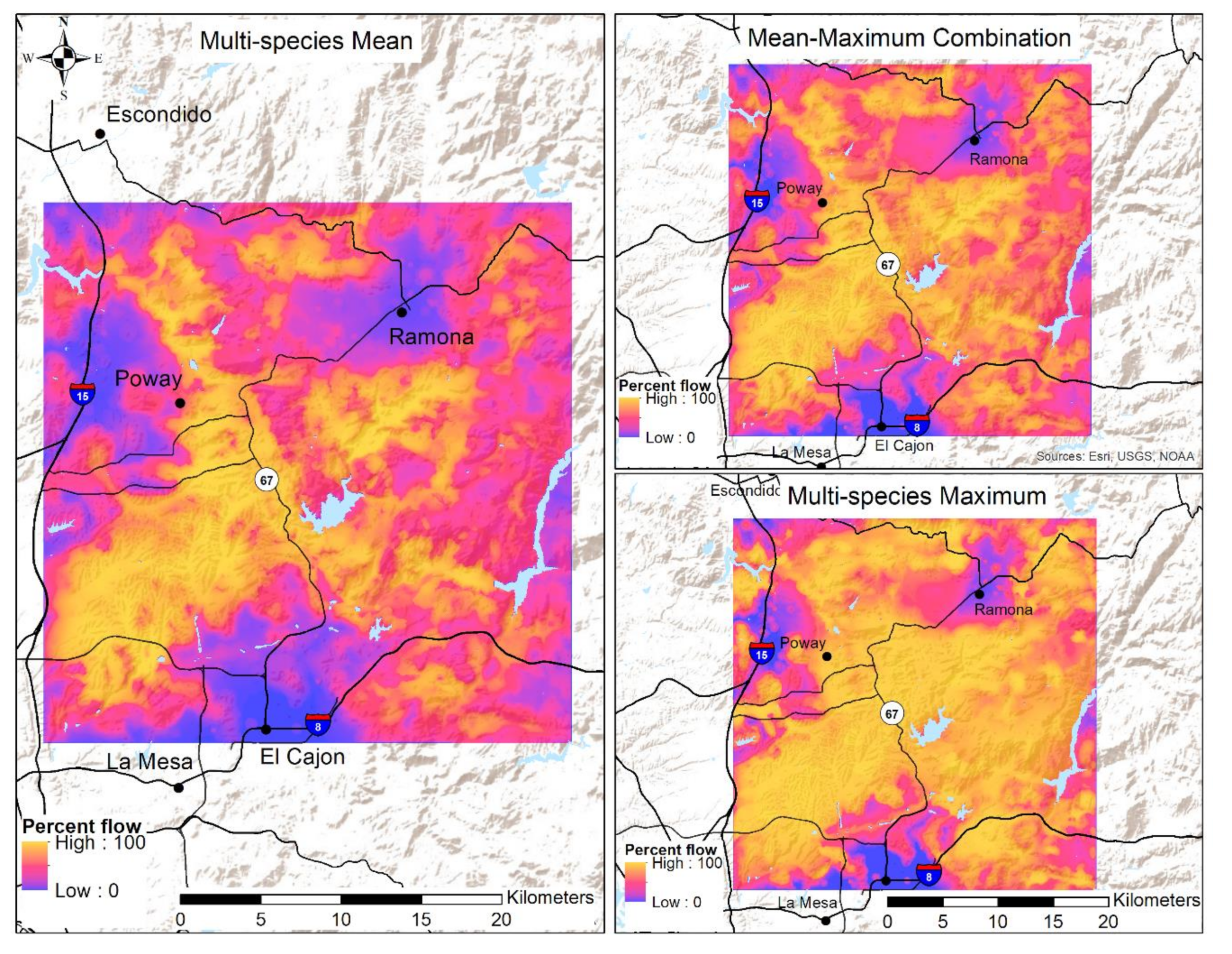
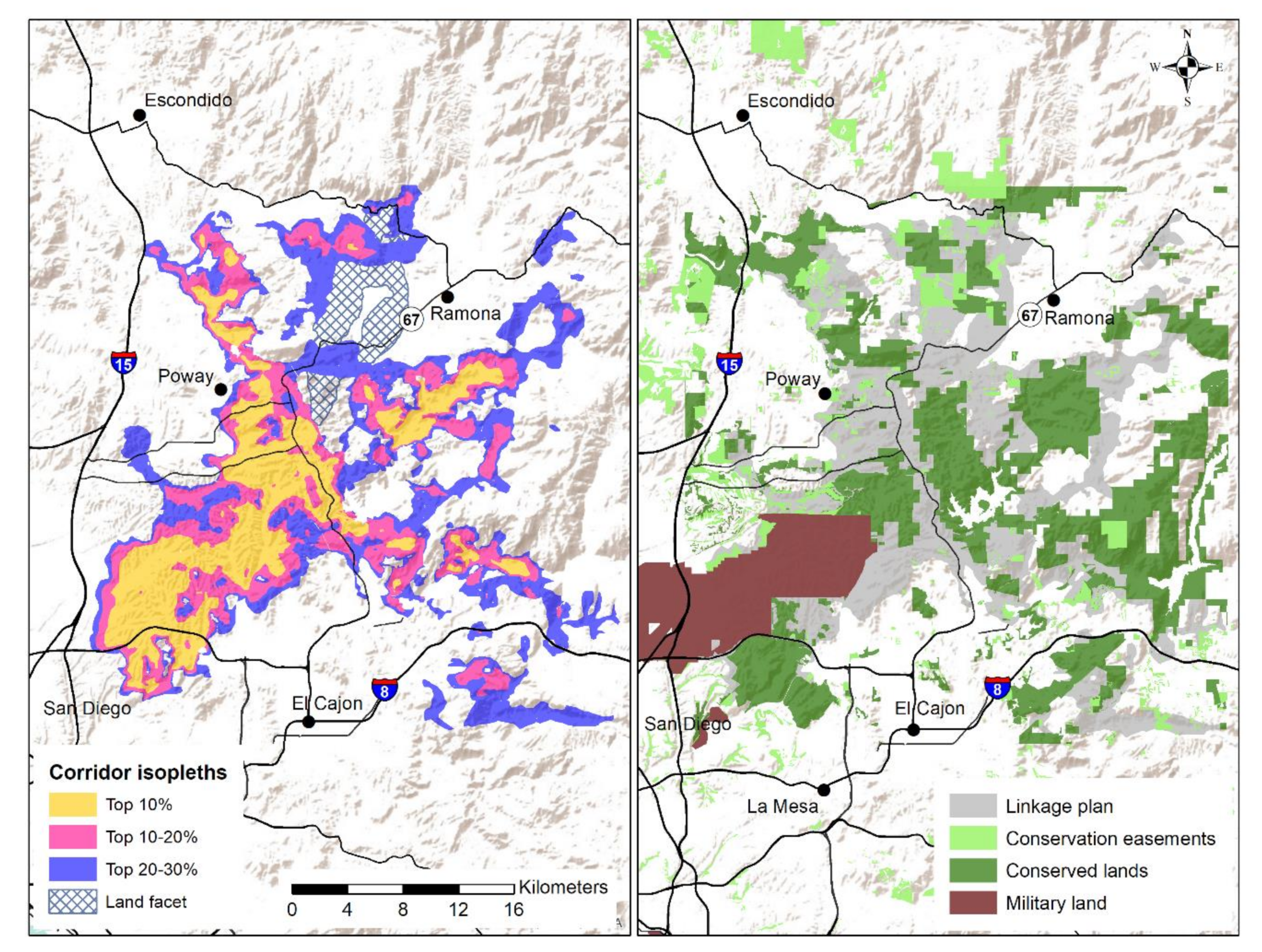
3.2. Connectivity Assessment

Between 1995 and 2017, the preserve network roughly doubled, growing from 142.5 km2 to 284.9 km2. However, cohesion and aggregation were lower compared with our outputs linking the preserve with corridors (Table 2). Our different corridor options would require the addition of another 249.9 to 525.0 km2 to the preserve network but would increase network cohesion and aggregation. Average corridor lengths and widths were relatively similar across the different multi-species linkages with the maximum flow approach resulting in the greatest improvement in connectivity metrics but requiring a nearly two-fold increase in conserved area. The comparison of approaches for developing a multi-species surface showed variation in flow value across the study area, as expected (Figure 3). The average surface had the lowest mean pixel value at 46.8% flow, followed by the mean–maximum combination at 62.1%, with the maximum surface having the highest mean pixel value at 74.5%. Despite the differences in mean pixel values, the correlation among layers was high, ranging from 0.88 to 0.98 with the greatest degree of correlation between the average and mean–maximum combination surfaces. Given the relative similarity of the highest connectivity value areas across all three approaches, we selected the averaging approach for our final connectivity surface because it was the most cost-effective option that still connected conserved lands within our study area.
The final multi-species linkage (Figure 4) connected lands from east to west and north to south across the study area and included a single land facet corridor. The linkage we assembled totaled 412 km2, which identified 206 km2 of previously unconserved lands for potential addition to the network, and another 206 km2 of lands that are under some degree of protection where management to promote or preserve connectivity may be needed. To facilitate interpretation and use of our data products in planning, we used a categorical symbology to display the final linkage (Figure 4) to distinguish between areas of top 10% of flow (90th percentile), 10–20% flow (80–90th percentile), and 20–30% flow (70–80th percentile).
Of the full linkage, 107 km2 fell within the top 10% of the flow value, 111 km2 in the top 10–20%, and 164 km2 in the top 20–30%. The land facet corridor was 30 km2 in area. The linkage encompassed high-quality habitats on conserved lands; 35% of the total linkage area is already conserved and 14% is prioritized for conservation under the regional conservation plan, the San Diego MSCP. Another 14% of the corridor overlapped with military or tribal lands, which are predominantly natural habitats but are not protected. The average resistant kernel flow across the combined multi-species surface was 81.5% for the multi-species linkage and 30.8% for the land facet linkage, which illustrates the need to combine approaches to incorporate important landscape features that may not be captured by selected focal species.
The final selected linkage provided for a high average flow value for each of the focal species (Figure A1) and had a high degree of overlap with the areas of highest connectivity value (≥50%) for each species (Figure 5). Had we relied only on structural connectivity—the null model, permeability, or the land facet analysis—we would have captured some of the key connectivity areas identified by our focal species models but would have greatly overestimated these areas. For example, with the land facet analysis, we would have identified 506 km2 for connectivity planning and implementation, with only 54.4% overlapping our multi-species linkage, excluding nearly 150 km2 of important connectivity area. If we used the top 30% of the resistant kernel flow surface based on landscape permeability to delineate the linkage, we would have mapped an area of 411 km2, with 245 km2 of that overlapping our multi-species linkage, excluding 175 km2 of important connectivity area (Figure 5).

4. Discussion

To ensure connectivity planning and implementation for protected area networks remain effective in the face of institutional and ecological changes, there is a pressing need to develop approaches that can evaluate, and where needed retrofit, existing networks with an adaptive framework. Using archived empirical data for six species, our comprehensive analysis combined a robust multi-species modeling approach, paired with a land facet analysis, to assess functional and structural connectivity in one of the first large-scale landscape plans established in the U.S., the San Diego MSCP, which has seen considerable changes in institutional and ecological conditions since its inception in 1996. Our study demonstrates how robust quantitative approaches can be employed to make use of available empirical data sources to assess functional and structural connectivity across protected area networks, leveraging the considerable investments from prior research and monitoring efforts for adaptive planning and management.
In the 25 years since the MSCP was first developed, there have been great strides towards meeting conservation goals, development of related plans, and a substantial increase in available data. However, concurrently, there have also been changes in land-use, increasing habitat fragmentation, proposed road widening plans, wildfires, and changes in ecological conditions that all affect the connectivity landscape. The multi-species approach we adopted allowed us to use existing species data to evaluate functional connectivity and a land facet analysis to assess structural connectivity to identify necessary linkages across the MSCP protected area network. Our analyses identified an additional 200 km2 of land that, if protected, could greatly improve connectivity in the MSCP. Our results highlight the power of combining a species-based approach with a species-agnostic land facet analysis [28,29] to capture both functional and structural connectivity. Specifically, the land facet analysis revealed the importance of grasslands linkages to connectivity within our study area, which were not represented by any of our focal species but are important for several rare and federally listed species.
A fundamental strength of our approach was the use of a wide range of empirical data types paired with appropriate analytical approaches. Although GPS telemetry data analyzed with point or path selection functions are often most representative of dispersal movements [21], we and others [66] found other data types such as occurrence and genetic data performed well for empirical connectivity analyses, particularly when appropriate resistance transformations are applied. In addition, we found that combining multiple data types for a single species, such as occurrence and genetic data, improved performance and representation of functional connectivity, as demonstrated by our analyses for mule deer (see Supplementary Materials S3). Although we conducted our connectivity assessment at the subregional scale where home range movements may be more constrained than dispersal movements, our approach to inform adaptive connectivity assessments for dynamic conditions can readily be scaled up with careful selection of focal species and integration of data types that include movement and genetic data.
A notable methodological aspect of our connectivity assessment was our comparison of results from two synoptic connectivity models—a cost distance approach [56] and an omnidirectional assessment of current flow [57]—which do not require a priori designation of habitat blocks or core areas. These models provided an opportunity to consider connectivity across the entire landscape, rather than just between protected areas. Such synoptic assessments may be particularly useful when assessing connectivity to adapt planning and management goals to changing ecological and institutional conditions, as they can be used to inform acquisition strategies as well as management actions to support and enhance connectivity. Because we did not observe substantial differences between the two connectivity modeling methods, future assessments may opt to employ only one approach, reducing analytical time.
Another important methodological aspect of our analysis was the evaluation of approaches to combine and present multiple, complex models. To ensure the connectivity assessment could be translated into targets for planning and management, we integrated our multi-species and landscape models into a single connectivity assessment map. Comparing approaches to create this integrated map (i.e., using average, maximum, or combined mean–maximum flow values), we found that averaging flows, the most area-restrictive approach, was most effective and cost-efficient for our planning environment (Table 2). The final linkage map we assembled identified areas with high connectivity value and a high degree of overlap across focal species which prioritized critical areas for functional connectivity that were not captured by land facets or landscape permeability.
Although our assessment relied on more complex analyses than those required to model connectivity based solely on landscape features or land cover, the methodology we developed can be applied to support a quantitative approach to connectivity planning and adaptive decision-making where survey and monitoring data are available. The ability to employ existing data can be particularly beneficial for rapid and iterative connectivity assessments without the investment of time and funding needed for the collection of the movement data frequently called for in traditional functional connectivity modeling [67,68]. While the individual connectivity modeling outputs we developed were static, by relying on existing, available data and combining those diverse data sources to assess both functional and structural connectivity, we demonstrate how this iterative approach can be used to help established protected areas adapt to ecological and institutional dynamics, and update plans accordingly. In our case, we put underutilized field data to work, capitalizing on prior investments in research and monitoring to rapidly assess connectivity in support of planning for future management of the protected area network while accounting for the changes that have occurred since plan inception. The combined multi-species and landscape modeling approach we adopted provided needed insight into both functional and structural connectivity, an important integration as our results suggest that connectivity assessments based on structural connectivity alone may be less likely to protect functional connectivity and require an equal or greater investment in land acquisition.

5. Conclusions

The empirical, multi-model analysis we describe is an efficient and cost-effective approach to inform adaptive planning for connectivity in established and new protected area networks over time. The empirical nature of our analysis, in particular, provides a strong foundation and quantitative justification for conservation actions that can be particularly useful for the crucial, but often overlooked, step of evaluating protected area network efficacy [1,26] and adapting plans accordingly. Our approach can also promote leveraging of existing data to establish new targets to enhance connectivity for protected area networks where implementation is ongoing but dynamic conditions affect the planning environment [69,70]. Paired with conservation stakeholder engagement and a thorough consideration of costs, conservation goals, as well as management priorities and challenges, this type of connectivity assessment using existing data can be used to guide and adapt decisions and actions on acquisitions, road crossings, management goals, and designation of appropriate multiple uses.

Supplementary Materials

The following are available online at https://www.mdpi.com/2073-445X/9/9/295/s1, Figure S1: Functions used to transform the environmental variables to resistance, with a range of 1-100, for use in the landscape genetic analysis, Table S1: Environmental variables used in developing habitat use and resistance surfaces for each focal species, Table S2: Variables and scales included in the final SDM models for California mouse, mule deer, woodrat, and wrentit. Variables without scales indicate it was not included in the final model for that species, Table S3: SDM model performance for California mouse, mule deer, woodrat, and wrentit. All models with an AUC > 0.75 were included in the final ensemble model. GLM = Generalized Linear Model, GAM = Generalized Additive Model, MARS = Multivariate adaptive regression splines, RF = Random forests, BRT = Boosted regression trees, Table S4: Variable scales, standardized beta estimates, robust standard errors, and 95% robust confidence intervals for the bobcat point selection function model-averaged variables, Table S5: Variable scales, standardized beta estimates, robust standard errors, and 95% robust confidence intervals for the puma point selection function variables, Table S6: Scales, standardized beta estimates, robust standard errors, and 95% robust confidence intervals for the bobcat path selection function model-averaged variables, Table S7: Scales, standardized beta estimates, robust standard errors, and 95% robust confidence intervals for the puma path selection function model-averaged variables, Table S8: Final model variables, scales and transformations to resistance for bobcat, mule deer, and puma. Variables without scales or transformations indicate it was not included in the final model for that species. Plus or minus indicates preference or avoidance of that variable for or movement. A forward slash refers to the inverse Ricker transformation, which indicates the lowest resistance values correspond with values in the middle of the range of values for that variable. The selected resistance transformation for the landscape genetic analysis are indicated by IR = inverse Ricker, NL = negative linear, NMCc = negative monomolecular concave, NMCv = negative monomolecular convex, PL = positive linear, PMCc = positive monomolecular concave, PMCv = positive monomolecular convex, Table S9: Description of the 15 different land facet types identified across the study area. The final selected land facet representing grasslands is identified in bold italics.

Author Contributions

Conceptualization, M.K.J., K.A.Z., and R.L.L.; methodology, M.K.J. and K.A.Z.; formal analysis, K.A.Z. and M.K.J.; data curation, M.K.J. and K.A.Z.; writing—original draft preparation, M.K.J.; writing—review and editing, K.A.Z. and R.L.L.; project administration, M.K.J.; funding acquisition, M.K.J. and R.L.L. All authors have read and agreed to the published version of the manuscript.

Funding

This research was funded by the San Diego Association of Governments, Agreement 5004388, Task Order 3.

Acknowledgments

We acknowledge those who shared data, including: W Vickers and W Boyce (University of California, Davis); H Ernest (University of Wyoming); A Vandergast, A Mitelberg, R Fisher, C Brehme, and K Preston (U.S. Geological Survey); S Tremor (San Diego Natural History Museum); M Tucker (Marine Corps Base Camp Pendleton); M Spiegelberg (Center for Natural Lands Management); R Botta (California Department of Fish and Wildlife). Comments on a prior draft of this manuscript by P Beier and five anonymous reviewers greatly improved this work.

Conflicts of Interest

The authors declare no conflict of interest.

Appendix A

Appendix A.1. Conservation Framework of San Diego’s Multiple Species Conservation Plan

In California, a combination of federal and state laws have been used to guide conservation planning since 1991 when the state passed the Natural Community Conservation Planning (NCCP) Act, designed to complement federal Habitat Conservation Plans (HCP) under the Endangered Species Act. The federal HCP and state NCCP approaches were intended to streamline permitting and approval processes for development projects while directing development to the lands where it will have minimal or reduced impacts, and to promote the protection of lands and waters of greatest conservation value. Since the mid-1990s, most new land preservation efforts in San Diego County have resulted from efforts to develop regional conservation networks for multiple species through HCPs required for incidental take permits issued under the federal ESA and under the authority of California’s NCCP. San Diego County led the way in these efforts between 1995 and 2005 with plans including the San Diego Multiple Species Conservation Plan (MSCP), which covers much of southwestern San Diego County. There are five subarea plans for each of the five jurisdictions that have approved implementing agreements under the MSCP. The plan covers 28 unique natural communities or land cover types, 38 animal species, and 42 plants. The plan is designed to be implemented over 50 years, which includes meeting conservation targets identified by the plan as well as conducting monitoring and management activities on core conserved lands.
Roughly three-quarters of our study area falls within the MSCP, with the remaining quarter overlapping a plan in process, the North County MSCP. Within our study area, there are nearly 215 km2 of protected areas, ~160 km2 of which have been conserved since 1980, in part because of the coordinated efforts to assemble the preserve network identified in the MSCP. Of these lands, some are managed as ecological preserves where access is limited, and priority is placed on protecting habitats and species. Many more conserved areas are managed as open spaces and park preserves where recreation is permitted but preservation of biodiversity is still prioritized. Finally, there are federal lands such as those managed by the Bureau of Land Management and the U.S. Forest Service, that are managed for multiple uses where protection of natural resources is one of several uses considered in making management decisions. In addition to these more formally conserved lands, there are tribal and military lands within our study area. Most of the area of these lands remains as open space and protected species and habitats are managed there. However, these lands are not part of the protected area network and a variety of activities or development that could fragment or disturb natural habitats and species may occur after appropriate environmental review. As such, although these lands include natural habitats and native species, they are not considered to have any kind of protected status.
Additional details, including planning documents and permits for the San Diego Multiple Species Conservation Plan can be found at:

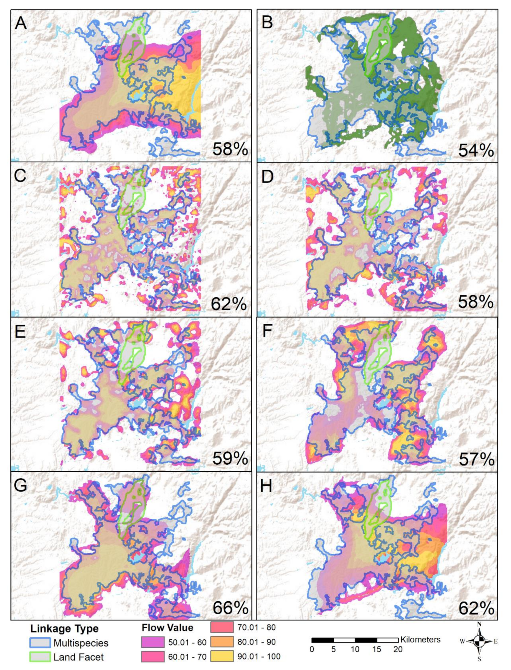
Appendix A.2. Multi-Species Flow Value Figure

To determine how well our multi-species linkage captured flow across the different connectivity surfaces, we calculated the mean flow value within the linkage area from the resistant kernel surfaces for the null model, permeability model, the mean species combination, and each individual focal species. Average flow ranged from 67.7% for puma to 75.1% for mule deer.
Figure A1. Box plot of the average resistant kernel connectivity flow value within the delineated multi-species linkage network for the null model, permeability-based model, mean multi-species surface as well as each individual species.
Land 09 00295 g0a1

References

  1. Boitani, L.; Falcucci, A.; Maiorano, L.; Rondinini, C. Ecological networks as conceptual frameworks or operational tools in conservation. Conserv. Biol. 2007, 21, 1414–1422. [Google Scholar] [CrossRef]
  2. Crooks, K.R.; Sanjayan, M. Connectivity Conservation Management; Cambridge University Press: Cambridge, UK, 2006; ISBN 9781849774727. [Google Scholar]
  3. Gilbert-Norton, L.; Wilson, R.; Stevens, J.R.; Beard, K.H. A Meta-Analytic Review of Corridor Effectiveness. Conserv. Biol. 2010, 24, 660–668. [Google Scholar] [CrossRef]
  4. Brown, J.H.; Kodric-Brown, A. Turnover Rates in Insular Biogeography: Effect of Immigration on Extinction. Ecology 1977, 58, 445–449. [Google Scholar] [CrossRef] [Green Version]
  5. Noss, R.F. Corridors in Real Landscapes: A Reply to Simberloff and Cox. Conserv. Biol. 1987, 1, 159–164. [Google Scholar] [CrossRef]
  6. Beier, P.; Noss, R.F. Do habitat corridors provide connectivity? Conserv. Biol. 1998, 12, 1241–1252. [Google Scholar] [CrossRef]
  7. Taylor, P.D.; Fahrig, L.; Henein, K.; Merriam, G. Connectivity Is a Vital Element of Landscape Structure. Oikos 1993, 68, 571. [Google Scholar] [CrossRef] [Green Version]
  8. Tischendorf, L.; Fahrig, L. On the usage and measurement of landscape connectivity. Oikos 2000, 90, 7–19. [Google Scholar] [CrossRef] [Green Version]
  9. Carter, S.K.; Januchowski-Hartley, S.R.; Pohlman, J.D.; Bergeson, T.L.; Pidgeon, A.M.; Radeloff, V.C. An evaluation of environmental, institutional and socio-economic factors explaining successful conservation plan implementation in the north-central United States. Biol. Conserv. 2015, 192, 135–144. [Google Scholar] [CrossRef]
  10. Jongman, R.H.G. Nature conservation planning in Europe: Developing ecological networks. Landsc. Urban Plan. 1995, 32, 169–183. [Google Scholar] [CrossRef]
  11. Convention on Biological Diversity. Decision UNEP/CBD/COP/DEC/X/2 Adopted by the Conference of the Parties to the Convention on Biological Diversity at its Tenth Meeting. 2011. Available online: https://www.cbd.int/decision/cop/?id=12268 (accessed on 16 July 2020).
  12. Saura, S.; Bertzky, B.; Bastin, L.; Battistella, L.; Mandrici, A.; Dubois, G. Global trends in protected area connectivity from 2010 to 2018. Biol. Conserv. 2019, 238, 108183. [Google Scholar] [CrossRef]
  13. Costello, C.; Polasky, S. Dynamic reserve site selection. Resour. Energy Econ. 2004, 26, 157–174. [Google Scholar] [CrossRef] [Green Version]
  14. Pressey, R.L.; Cabeza, M.; Watts, M.E.; Cowling, R.M.; Wilson, K.A. Conservation planning in a changing world. Trends Ecol. Evol. 2007, 22, 583–592. [Google Scholar] [CrossRef] [PubMed]
  15. Van Teeffelen, A.J.A.; Vos, C.C.; Opdam, P. Species in a dynamic world: Consequences of habitat network dynamics on conservation planning. Biol. Conserv. 2012, 153, 239–253. [Google Scholar] [CrossRef] [Green Version]
  16. Opdam, P.; Steingröver, E.; van Rooij, S. Ecological networks: A spatial concept for multi-actor planning of sustainable landscapes. Landsc. Urban Plan. 2006, 75, 322–332. [Google Scholar] [CrossRef]
  17. Fagan, W.F.; Calabrese, J.M. Quantifying connectivity: Balancing metric performance with data requirements. In Connectivity Conservation; Crooks, K.R., Sanjayan, M., Eds.; Cambridge University Press: Cambridge, UK, 2006; pp. 297–317. ISBN 9780521857062. [Google Scholar]
  18. Kool, J.T.; Moilanen, A.; Treml, E.A. Population connectivity: Recent advances and new perspectives. Landsc. Ecol. 2013, 28, 165–185. [Google Scholar] [CrossRef]
  19. Epps, C.W.; Mutayoba, B.M.; Gwin, L.; Brashares, J.S. An empirical evaluation of the African elephant as a focal species for connectivity planning in East Africa. Divers. Distrib. 2011, 17, 603–612. [Google Scholar] [CrossRef]
  20. McClure, M.L.; Hansen, A.J.; Inman, R.M. Connecting models to movements: Testing connectivity model predictions against empirical migration and dispersal data. Landsc. Ecol. 2016, 31, 1419–1432. [Google Scholar] [CrossRef]
  21. Zeller, K.A.; Jennings, M.K.; Vickers, T.W.; Ernest, H.B.; Cushman, S.A.; Boyce, W.M. Are all data types and connectivity models created equal? Validating common connectivity approaches with dispersal data. Divers. Distrib. 2018, 24, 868–879. [Google Scholar] [CrossRef] [Green Version]
  22. Naidoo, R.; Kilian, J.W.; Du Preez, P.; Beytell, P.; Aschenborn, O.; Taylor, R.D.; Stuart-Hill, G. Evaluating the effectiveness of local- and regional-scale wildlife corridors using quantitative metrics of functional connectivity. Biol. Conserv. 2018, 217, 96–103. [Google Scholar] [CrossRef]
  23. Sanderson, E.W.; Redford, K.H.; Vedder, A.; Coppolillo, P.B.; Ward, S.E. A conceptual model for conservation planning based on landscape species requirements. Landsc. Urban Plan. 2002, 58, 41–56. [Google Scholar] [CrossRef]
  24. Lambeck, R.J. Focal species: A multi-species umbrella for nature conservation. Conserv. Biol. 1997, 11, 849–856. [Google Scholar] [CrossRef] [Green Version]
  25. Dilkina, B.; Houtman, R.; Gomes, C.P.; Montgomery, C.A.; McKelvey, K.S.; Kendall, K.; Graves, T.A.; Bernstein, R.; Schwartz, M.K. Trade-offs and efficiencies in optimal budget-constrained multispecies corridor networks. Conserv. Biol. 2017, 31, 192–202. [Google Scholar] [CrossRef] [PubMed]
  26. Gippoliti, S.; Battisti, C. More cool than tool: Equivoques, conceptual traps and weaknesses of ecological networks in environmental planning and conservation. Land Use Policy 2017, 68, 686–691. [Google Scholar] [CrossRef]
  27. Albert, C.H.; Rayfield, B.; Dumitru, M.; Gonzalez, A. Applying network theory to prioritize multispecies habitat networks that are robust to climate and land-use change. Conserv. Biol. 2017, 31, 1383–1396. [Google Scholar] [CrossRef] [PubMed] [Green Version]
  28. Brost, B.M.; Beier, P. Comparing linkage designs based on land facets to linkage designs based on focal species. PLoS ONE 2012, 7, e48965. [Google Scholar] [CrossRef] [Green Version]
  29. Krosby, M.; Breckheimer, I.; Pierce, D.J.; Singleton, P.H.; Hall, S.A.; Halupka, K.C.; Gaines, W.L.; Long, R.A.; McRae, B.H.; Cosentino, B.L.; et al. Focal species and landscape “naturalness” corridor models offer complementary approaches for connectivity conservation planning. Landsc. Ecol. 2015, 30, 2121–2132. [Google Scholar] [CrossRef]
  30. Anderson, M.G.; Comer, P.J.; Beier, P.; Lawler, J.J.; Schloss, C.A.; Buttrick, S.; Albano, C.M.; Faith, D.P. Case studies of conservation plans that incorporate geodiversity. Conserv. Biol. 2015, 29, 680–691. [Google Scholar] [CrossRef]
  31. Beier, P.; Brost, B. Use of land facets to plan for climate change: Conserving the arenas, not the actors. Conserv. Biol. 2010, 24, 701–710. [Google Scholar] [CrossRef]
  32. Theobald, D.M.; Reed, S.E.; Fields, K.; Soulé, M. Connecting natural landscapes using a landscape permeability model to prioritize conservation activities in the United States. Conserv. Lett. 2012, 5, 123–133. [Google Scholar] [CrossRef]
  33. Greer, K.A. Habitat Conservation Planning in San Diego County, California: Lessons Learned After Five Years of Implementation. Environ. Pract. 2004, 6, 230–239. [Google Scholar] [CrossRef]
  34. Beier, P.; Penrod, K.; Luke, C.; Spencer, W.; Cabañero, C. South Coast missing linkages: Restoring connectivity to wildlands in the largest metropolitan area in the United States. In Connectivity Conservation; Crooks, K.R., Sanjayan, M.A., Eds.; Cambridge University Press: Cambridge, UK, 2006; pp. 555–586. [Google Scholar]
  35. South Coast Wildlands. South Coast Missing Linkages: A Wildland Network for the South Coast Ecoregion. 2008. Available online: http://www.scwildlands.org/reports/SCMLRegionalReport.pdf (accessed on 16 July 2020).
  36. Spencer, W.D.; Beier, P.; Penrod, K.; Paulman, K.; Rustigian-Romsos, H.; Strittholt, J.; Parisi, M.; Pettler, A. California Essential Habitat Connectivity Project: A Strategy for Conservation a Connected California; 2010. Available online: https://nrm.dfg.ca.gov/FileHandler.ashx?DocumentID=18366 (accessed on 16 July 2020).
  37. Crooks, K.R. Relative sensitivities of mammalian carnivores to habitat fragmentation. Conserv. Biol. 2002, 16, 488–502. [Google Scholar] [CrossRef]
  38. Mitelberg, A.; Vandergast, A.G. Non-Invasive Genetic Sampling of Southern Mule Deer (Odocoileus hemionus fuliginatus) Reveals Limited Movement Across California State Route 67 in San Diego County. West. Wildl. 2016, 3, 8–18. [Google Scholar]
  39. Baker, M.; Nur, N.; Geupel, G.R. Correcting biased estimates of dispersal and survival due to limited study area: Theory and an application using wrentits. Condor 1995, 97, 663–674. [Google Scholar] [CrossRef]
  40. Mendelsohn, M.B.; Brehme, C.S.; Rochester, C.J.; Stokes, D.C.; Hathaway, S.A.; Fisher, R.N. Responses in bird communities to wildland fires in southern California. Fire Ecol. Spec. Issue 2008, 4, 63–82. [Google Scholar] [CrossRef]
  41. Delaney, K.S.; Riley, S.P.D.; Fisher, R.N. A rapid, strong, and convergent genetic response to urban habitat fragmentation in four divergent and widespread vertebrates. PLoS ONE 2010, 5, 1–11. [Google Scholar] [CrossRef] [Green Version]
  42. Tremor, S.; Stokes, D.; Spencer, W.; Diffendorfer, J.; Thomas, H.; Chivers, S.; Unitt, P. San Diego County Mammal Atlas. In San Diego Society of Natural History, 46th ed.; San Diego Natural History Museum: San Diego, CA, USA, 2017; ISBN 9780692895399. [Google Scholar]
  43. County of San Diego SanBIOS Biological Database. Available online: http://rdw.sandag.org/Account/GetFSFile.aspx?dir=Ecology&Name=SanBIOS.zip (accessed on 21 October 2016).
  44. Ebird Ebird: An Online Database of Bird Distribution and Abundance [Web Application]. Available online: http://www.ebird.org (accessed on 28 December 2016).
  45. Jennings, M.K.; Lewison, R.L. Planning for Connectivity under Climate Change: Using Bobcat Movement to Assess Landscape Connectivity across San Diego County’s Open Spaces; San Diego State University: San Diego, CA, USA, 2013. [Google Scholar]
  46. San Diego Management and Monitoring Program Master Occurrence Matrix Database. Available online: https://www.sciencebase.gov/catalog/item/53e27963e4b0fe532be3bddf (accessed on 28 December 2016).
  47. Ernest, H.B.; Vickers, T.W.; Morrison, S.A.; Buchalski, M.R.; Boyce, W.M. Fractured Genetic Connectivity Threatens a Southern California Puma (Puma concolor) Population. PLoS ONE 2014, 9, e107985. [Google Scholar] [CrossRef] [Green Version]
  48. Zeller, K.A.; McGarigal, K.; Cushman, S.A.; Beier, P.; Vickers, T.W.; Boyce, W.M. Using step and path selection functions for estimating resistance to movement: Pumas as a case study. Landsc. Ecol. 2016, 31, 1319–1335. [Google Scholar] [CrossRef]
  49. Johnson, C.J.; Seip, D.R.; Boyce, M.S. A quantitative approach to conservation planning: Using resource selection functions to map the distribution of mountain caribou at multiple spatial scales. J. Appl. Ecol. 2004, 41, 238–251. [Google Scholar] [CrossRef]
  50. McGarigal, K.; Wan, H.Y.; Zeller, K.A.; Timm, B.C.; Cushman, S.A. Multi-scale habitat selection modeling: A review and outlook. Landsc. Ecol. 2016, 31, 1161–1175. [Google Scholar] [CrossRef]
  51. Adriaensen, F.; Chardon, J.P.; De Blust, G.; Swinnen, E.; Villalba, S.; Gulinck, H.; Matthysen, E. The application of ‘least-cost’ modelling as a functional landscape model. Landsc. Urban Plan. 2003, 64, 233–247. [Google Scholar] [CrossRef]
  52. Zeller, K.A.; Vickers, T.W.; Ernest, H.B.; Boyce, W.M. Multi-level, multi-scale resource selection functions and resistance surfaces for conservation planning: Pumas as a case study. PLoS ONE 2017, 12, e0179570. [Google Scholar] [CrossRef] [PubMed]
  53. Keeley, A.T.H.; Beier, P.; Gagnon, J.W. Estimating landscape resistance from habitat suitability: Effects of data source and nonlinearities. Landsc. Ecol. 2016, 31, 2151–2162. [Google Scholar] [CrossRef]
  54. Trainor, A.M.; Walters, J.R.; Morris, W.F.; Sexton, J.; Moody, A. Empirical estimation of dispersal resistance surfaces: A case study with red-cockaded woodpeckers. Landsc. Ecol. 2013, 28, 755–767. [Google Scholar] [CrossRef]
  55. Mateo-Sánchez, M.C.; Balkenhol, N.; Cushman, S.; Pérez, T.; Domínguez, A.; Saura, S. A comparative framework to infer landscape effects on population genetic structure: Are habitat suitability models effective in explaining gene flow? Landsc. Ecol. 2015, 30, 1405–1420. [Google Scholar] [CrossRef]
  56. Compton, B.W.; McGarigal, K.; Cushman, S.A.; Gamble, L.R. A resistant-kernel model of connectivity for amphibians that breed in vernal pools. Conserv. Biol. 2007, 21, 788–799. [Google Scholar] [CrossRef]
  57. McRae, B.H.; Popper, K.; Jones, A.; Schindel, M.; Buttrick, S.; Hall, K.; Unnasch, R.S.; Platt, J. Conserving Nature’s Stage: Mapping Omnidirectional Connectivity for Resilient Terrestrial Landscapes in the Pacific Northwest; The Nature Conservancy: Portland, OR, USA, 2016. [Google Scholar]
  58. Landguth, E.L.; Hand, B.K.; Glassy, J.; Cushman, S.A.; Sawaya, M.A. UNICOR: A species connectivity and corridor network simulator. Ecography 2012, 35, 9–14. [Google Scholar] [CrossRef]
  59. Ribble, D.O. Dispersal in a monogamous rodent, Peromyscus californicus. Ecology 1992, 73, 859–866. [Google Scholar] [CrossRef] [Green Version]
  60. Beier, P. Dispersal of juvenile cougars in fragmented habitat. J. Wildl. Manag. 1995, 59, 228. [Google Scholar] [CrossRef]
  61. Smith, M.H. Dispersal capacity of the dusky-footed woodrat, Neotoma fuscipes. Am. Midl. Nat. 1965, 74, 457. [Google Scholar] [CrossRef]
  62. Beier, P.; Majka, D.R.; Spencer, W.D. Forks in the road: Choices in procedures for designing wildland linkages. Conserv. Biol. 2008, 22, 836–851. [Google Scholar] [CrossRef]
  63. Hesselbarth, M.H.K.; Sciaini, M.; With, K.A.; Wiegand, K.; Nowosad, J. Landscapemetrics: An open-source R tool to calculate landscape metrics. Ecography 2019, 42, 1648–1657. [Google Scholar] [CrossRef] [Green Version]
  64. Jin, S.; Yang, L.; Danielson, P.; Homer, C.; Fry, J.; Xian, G. A comprehensive change detection method for updating the National Land Cover Database to circa 2011. Remote Sens. Environ. 2013, 132, 159–175. [Google Scholar] [CrossRef] [Green Version]
  65. Buttrick, S.; Popper, K.; McRae, B.; Unnasch, B.; Schindel, M.; Jones, A.; Platt, J. Conserving Nature’s Stage: Identifying Resilient Terrestrial Landscapes in the Pacific Northwest; Portland, OR, USA. 2015. Available online: http://nature.ly/resilienceNW (accessed on 18 October 2019).
  66. Valerio, F.; Carvalho, F.; Barbosa, A.M.; Mira, A.; Santos, S.M. Accounting for Connectivity Uncertainties in Predicting Roadkills: A Comparative Approach between Path Selection Functions and Habitat Suitability Models. Environ. Manag. 2019, 64, 329–343. [Google Scholar] [CrossRef] [PubMed] [Green Version]
  67. Keeley, A.T.H.; Beier, P.; Keeley, B.W.; Fagan, M.E. Habitat suitability is a poor proxy for landscape connectivity during dispersal and mating movements. Landsc. Urban Plan. 2017, 161, 90–102. [Google Scholar] [CrossRef]
  68. Abrahms, B.; Sawyer, S.C.; Jordan, N.R.; McNutt, J.W.; Wilson, A.M.; Brashares, J.S. Does wildlife resource selection accurately inform corridor conservation? J. Appl. Ecol. 2017, 54, 412–422. [Google Scholar] [CrossRef] [Green Version]
  69. Santini, L.; Saura, S.; Rondinini, C. Connectivity of the global network of protected areas. Divers. Distrib. 2016, 22, 199–211. [Google Scholar] [CrossRef] [Green Version]
  70. Saura, S.; Bastin, L.; Battistella, L.; Mandrici, A.; Dubois, G. Protected areas in the world’s ecoregions: How well connected are they? Ecol. Indic. 2017, 76, 144–158. [Google Scholar] [CrossRef]
Figure 1. Map of the study area in San Diego County, CA, USA. The box delineates the analysis area for the project area. Map depicts conserved lands established before and after the preserve network was established in 1996, conservation easements, and military lands that are largely undeveloped. Inset shows location of the county and study area in a statewide context.
Land 09 00295 g001
Figure 2. Flowchart of the methodological approach for modeling corridors using complementary approaches to identify a single corridor network based on multiple focal species and multiple modeling methods. The top panel depicts analytical steps to obtain a resistance surface and the bottom panel details how data were processed for individual species and then synthesized into a single, multi-species surface. The point selection function that was used to generate source points for connectivity modeling across probability of movement surfaces is not depicted. The genetic resistance surface was combined with the species distribution model (SDM) resistance surface for mule deer and the path selection function resistance surfaces for puma and bobcat.
Land 09 00295 g002
Figure 3. Comparison of different approaches to multi-species connectivity surface assembly. The left panel represents the average percent flow across all six focal species; lower right shows the maximum percent flow for any given species at each pixel; top right shows the result of combining the average and maximum flow values.
Land 09 00295 g003
Figure 4. Connectivity outputs from the multi-species analysis. Left panel depicts the top 30% of flow for connectivity with isopleths identifying the top 10%, the top 10–20%, and the top 20–30% with increasing levels of saturation. The land facet linkage is identified by cross-hatching. The right panel shows the addition of the spatially explicit linkage, which connects conserved lands and conservation easements from the protected area network, as well as undeveloped areas on military lands.
Land 09 00295 g004
Figure 5. Spatial overlap among the multi-species linkage and individual connectivity surfaces based on: (A) permeability, (B) land facet, (C) California mouse, (D) big-eared woodrat, (E) wrentit, (F) bobcat, (G) mule deer, and (H) puma. All panels except the land facet depict the top 50% of resistant kernel flow, whereas the land facet, in dark green, is a union of linkages modeled from the 15 different land facet categories. The percent of spatial overlap for each surface is noted in the lower right corner of each panel.
Land 09 00295 g005
Table 1. Focal species, available data types, data sources, and analytical models used in the analysis.
Focal Species (Scientific Name)Data Type(s)Data Source(s)Analytical Method(s)
California mouse (Peromyscus californicus)Occurrence pointsSDNHM Mammal Atlas 1, SanBIOS 2Species Distribution Model
Big-eared woodrat (Neotoma macrotis)Occurrence pointsSDNHM Mammal Atlas 1, SanBIOS 2Species Distribution Model
Wrentit (Chamaea fasciata)Occurrence pointseBIRD 3Species Distribution Model
Mule deer (Odocoileus hemionus californicus)Occurrence points and genetic dataSDNHM Mammal Atlas 1, SanBIOS 2, SDSU 4, SDMMP MOM 5, USGS 6Species Distribution Model and Landscape genetics analysis
Bobcat (Lynx rufus)GPS telemetry and genetic dataSDSU 4Resource and Movement Selection Functions and Landscape genetics analysis
Puma (Puma concolor)GPS telemetry and genetic dataUniversity of California, Davis 7Resource and Movement Selection Functions and Landscape genetics analysis
1 San Diego Natural History Museum (SDNHM) Mammal Atlas [42];2 SanBIOS Dataset [43]; 3 eBird [44]; 4 San Diego State University [45]; 5 San Diego Management and Monitoring Program Master Occurrence Matrix [46]; 6 United States Geological Survey (USGS; [38]);7 University of California, Davis [47,48].
Table 2. Metrics describing the size and connectivity of the preserve network in 1995 and 2017 (in italics), the linkage options evaluated for resistant kernel flow surfaces to combine connectivity for multiple species and the final combined linkage (in bold), which included additional area from the Omniscape and land facet analyses. Area describes the size of the preserve network in 1995 and 2017, and for the four linkage options, the additional land needed to complete the network. Mean corridor length and width values were calculated based on distances to connect existing preserve lands. Aggregation and cohesion indices were calculated at the landscape scale. No corridor length or width metrics were calculated for the preserve in 1995 or 2017 because no spatially explicit linkages were delineated for the network prior to this analysis.
Area (km2)Mean Corridor Length (km)Mean Corridor Width (km)Aggregation(%)Cohesion(%)
Preserve in 1995142.5 96.298.8
Preserve in 2017284.9 96.699.0
Combined multi-species linkage269.512.72.198.599.9
Average multi-species linkage249.912.82.198.499.9
Mean–max multi-species linkage339.716.2298.799.9
Maximum multi-species linkage525.012.72.299.3100.0

