Spatio-Temporal Dynamics of Landscape Connectivity and Ecological Network Construction in Long Yangxia Basin at the Upper Yellow River


Abstract
:1. Introduction
2. Materials and Methods
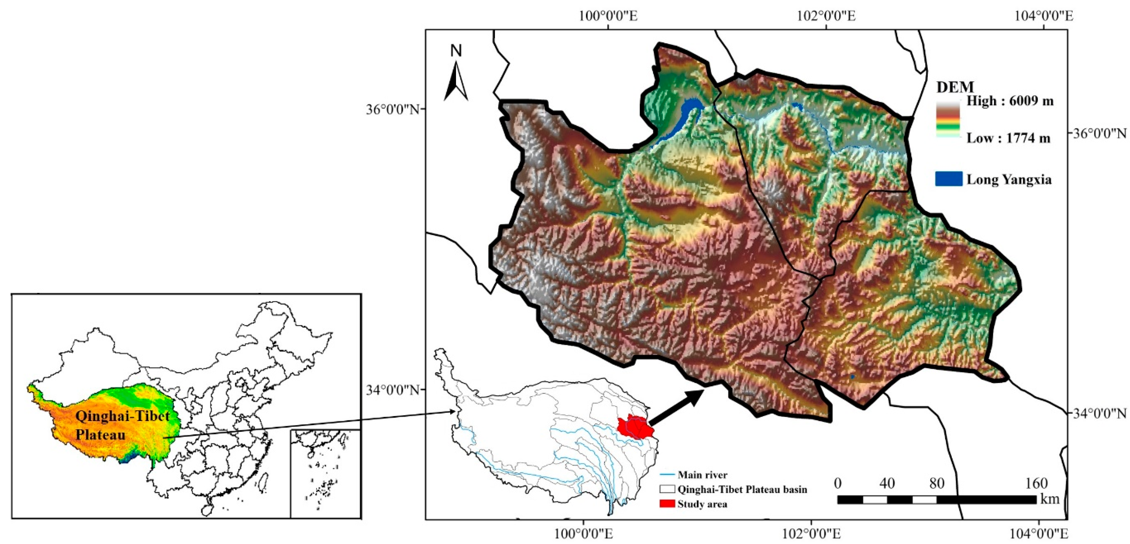
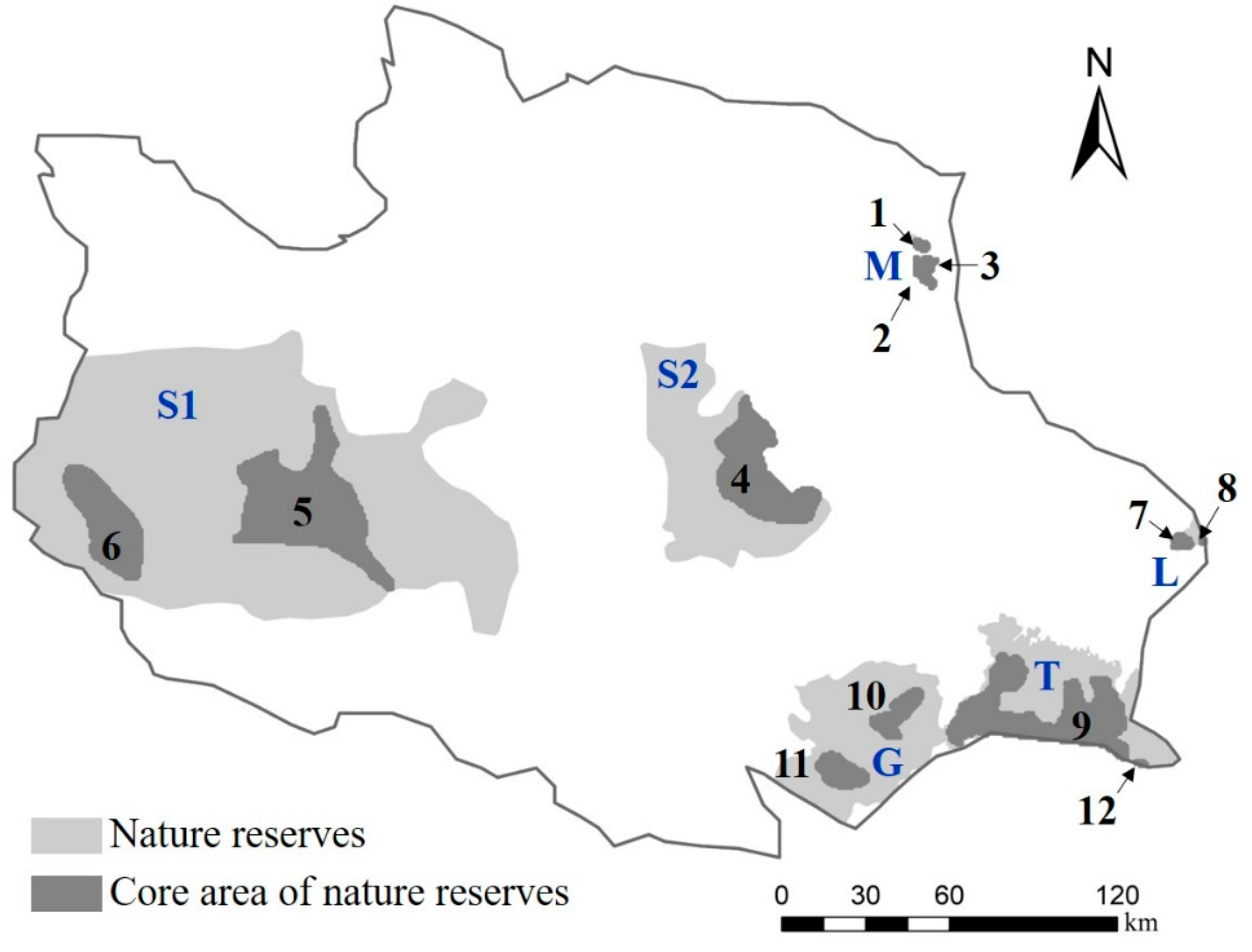
2.1. Study Area
2.2. Data Sources
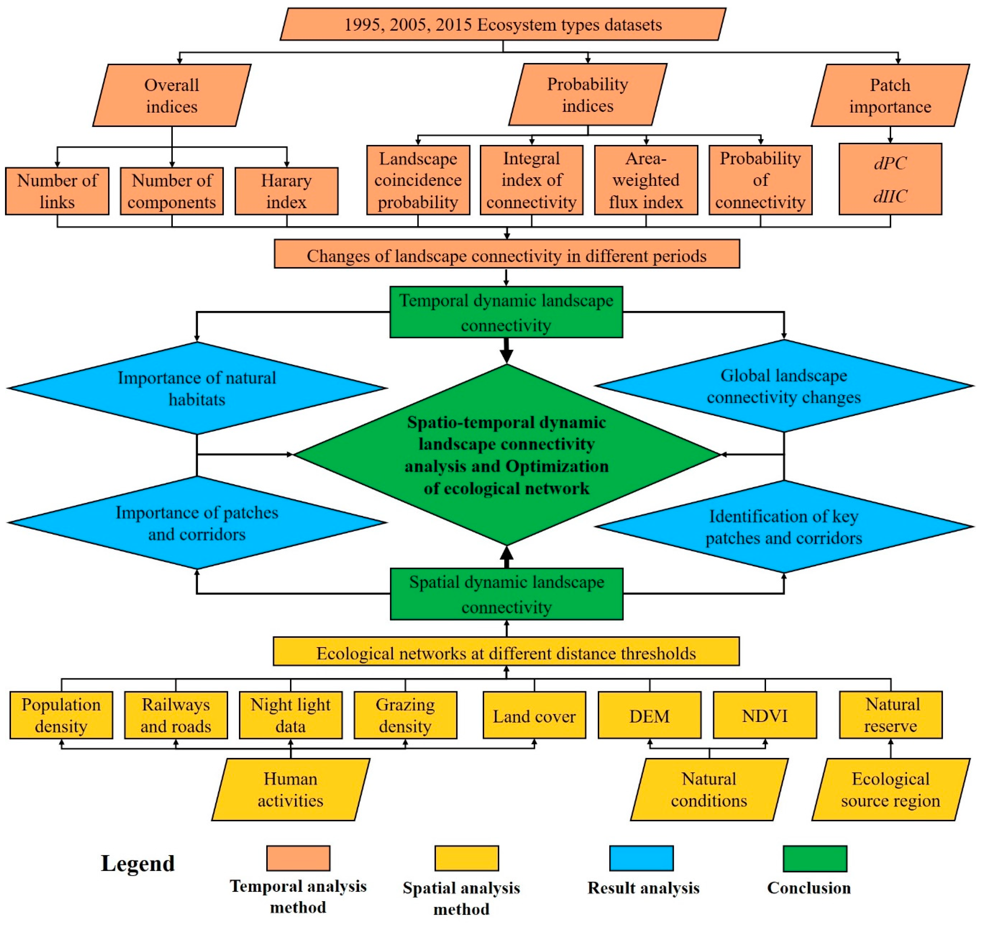
2.3. Data Analysis
2.3.1. Global Landscape Connectivity Assessment
2.3.2. The Evaluation of the Importance of Natural Habitats
2.3.3. The Construction of Ecological Network
Determination of Ecological Source Regions and Resistance Surface
Minimum Cumulative Resistance Model
2.3.4. Analysis of Ecological Network Connectivity and the Importance of Patches and Corridors
3. Results
3.1. Temporal Dynamics of Landscape Connectivity
3.1.1. Changes in the Global Connectivity
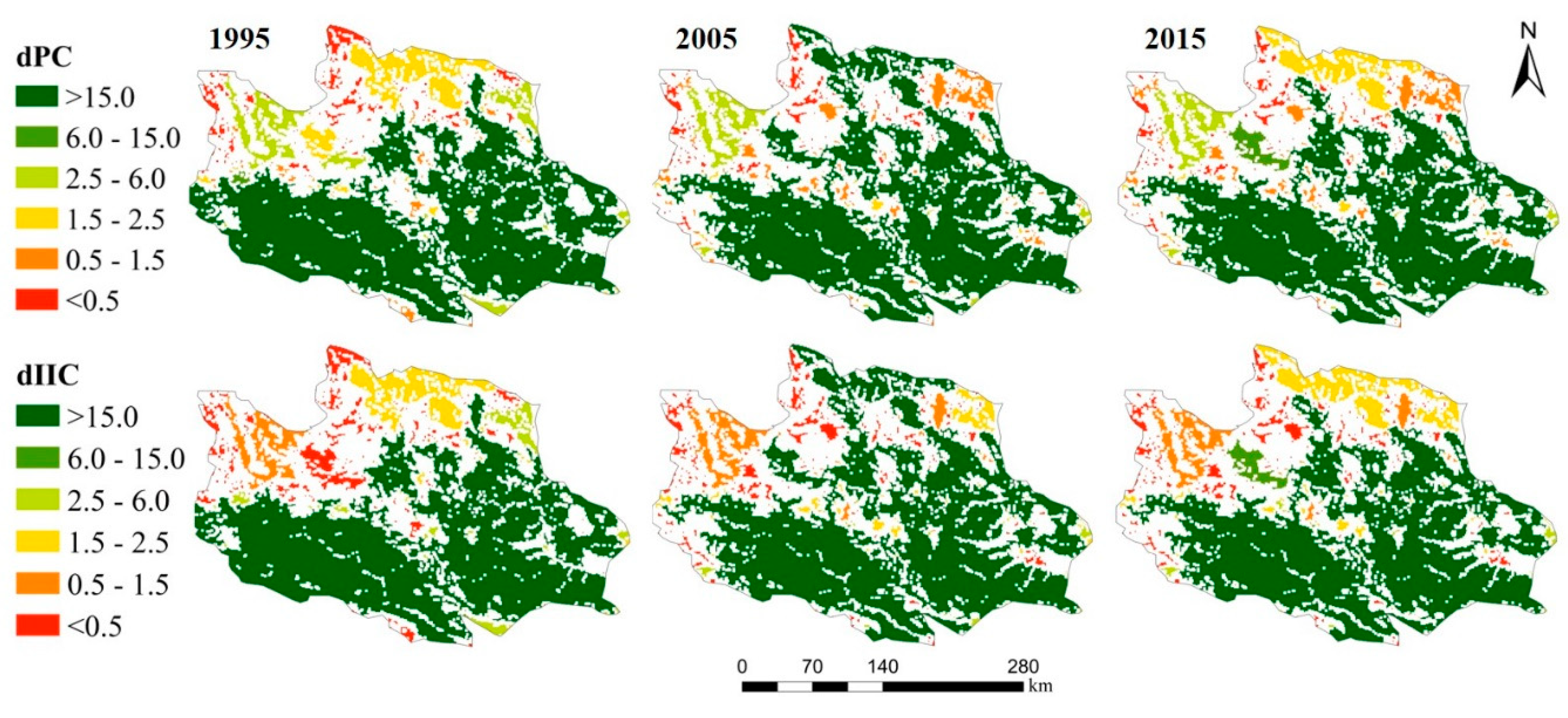
3.1.2. Changes in the Importance of Natural Habitats
3.2. Spatial Dynamics in Landscape Connectivity
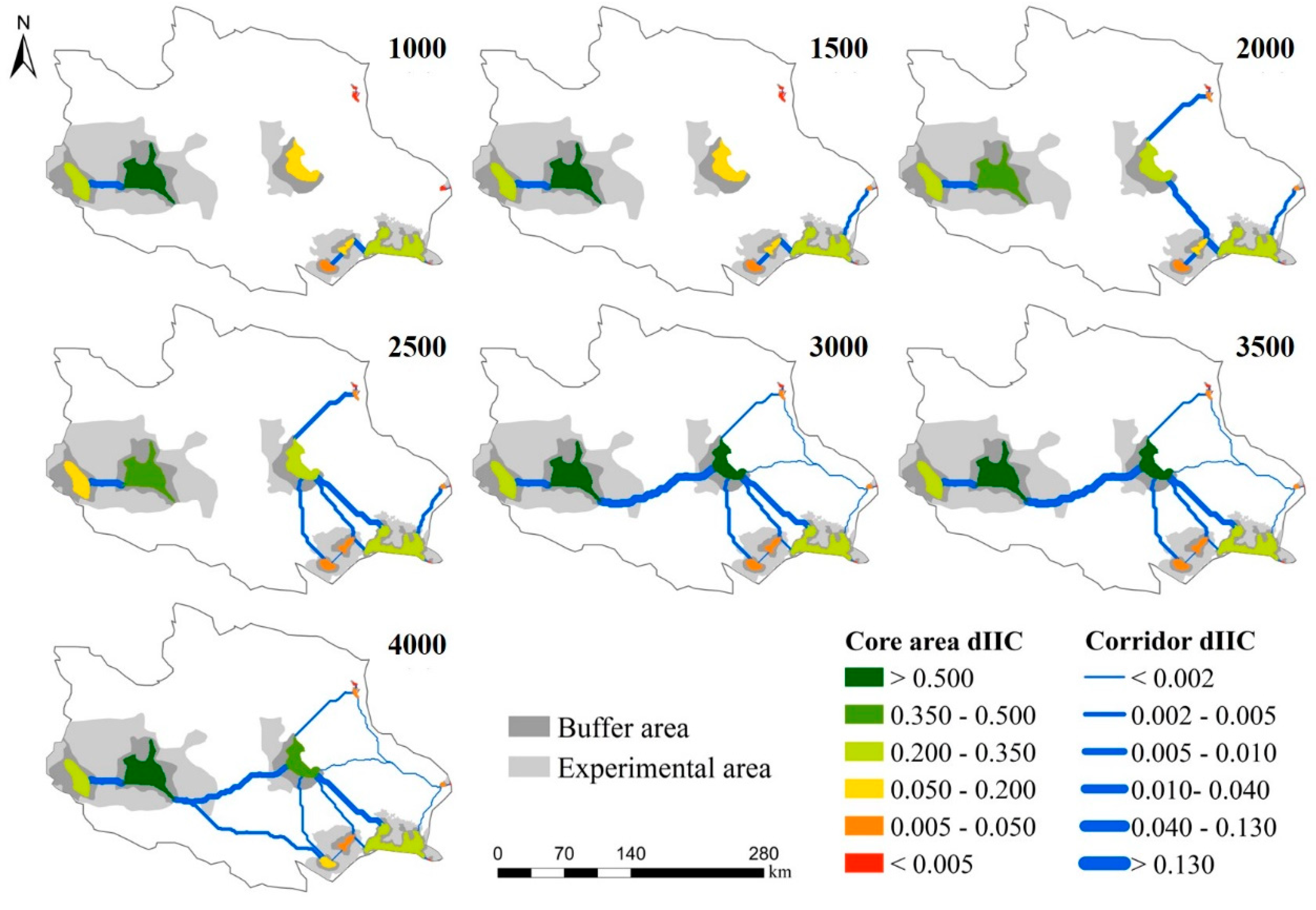
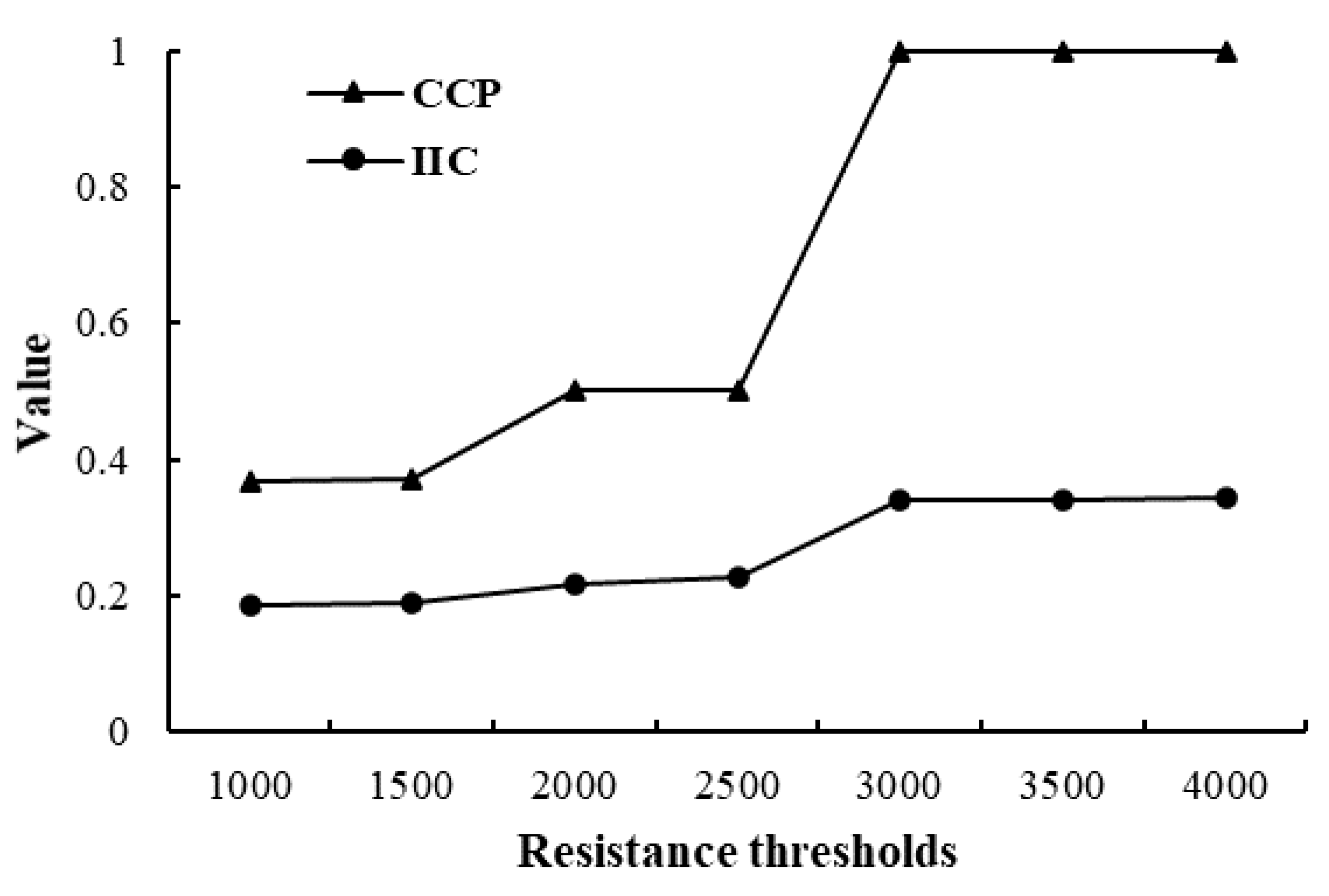
3.2.1. Construction of Ecological Network under Different Distance Thresholds
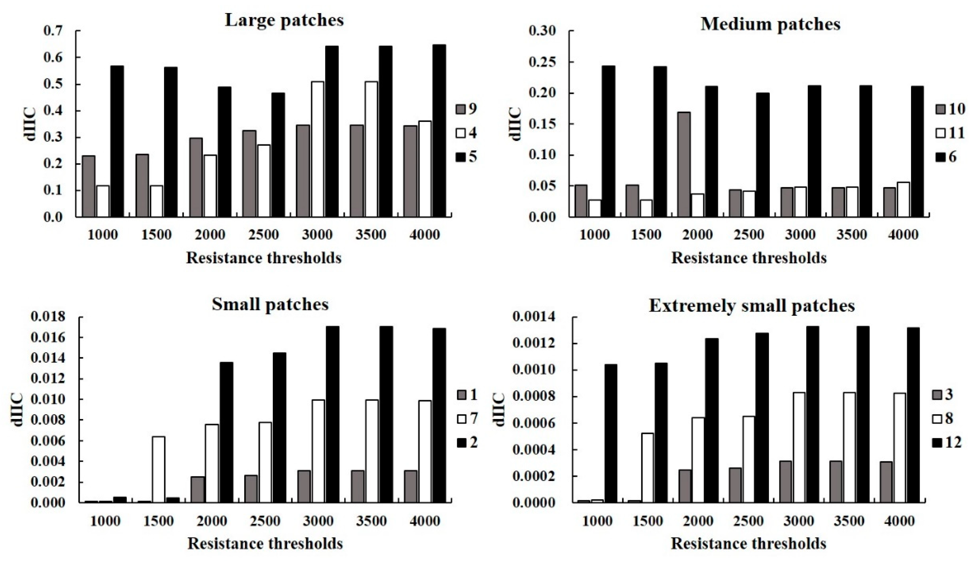
3.2.2. Analysis of the Importance of Patches and Corridors
3.3. Analysis of Buffer Zone of Potential Ecological Corridor
4. Discussion
4.1. Spatio-Temporal Dynamic Landscape Connectivity Analysis
4.2. Identification of Key Areas and Optimization of Landscape Pattern
5. Conclusions
Author Contributions
Funding
Conflicts of Interest
References
- Benton, T.; Vickery, J.; Wilson, J. Farmland biodiversity: Is habitat heterogeneity the key? Trends Ecol. Evol. 2003, 18, 182–188. [Google Scholar] [CrossRef]
- Butler, S.; Vickery, J.; Norris, K. Farmland biodiversity and the footprint of agriculture. Science 2007, 315, 381–384. [Google Scholar] [CrossRef] [PubMed]
- Mao, D.H.; Luo, L.; Wang, Z.M.; Wilson, M.; Zeng, Y.; Wu, B.F.; Wu, J.G. Conversions between natural wetlands and farmland in China: A multiscale geospatial analysis. Sci. Total Environ. 2018, 634, 550–560. [Google Scholar] [CrossRef] [PubMed]
- Liu, S.L.; Yin, Y.J.; Cheng, F.Y.; Hou, X.Y.; Dong, S.K.; Wu, X. Spatio-temporal variations of conservation hotspots based on ecosystem services in Xishuangbanna, Southwest China. PLoS ONE 2017, 12, e0189368. [Google Scholar] [CrossRef] [PubMed] [Green Version]
- Baranyi, G.; Saura, S.; Jordán, F. Contribution of habitat patches to network connectivity: Redundancy and uniqueness of topological indices. Ecol. Indic. 2011, 11, 1301–1310. [Google Scholar] [CrossRef]
- Loro, M.; Pérez, E.; Arce-Ruiz, R.; Geneletti, D. Ecological connectivity analysis to reduce the barrier effect of roads. An innovative graph-theory approach to define wildlife corridors with multiple paths and without bottlenecks. Landsc. Urban Plan. 2015, 139, 149–162. [Google Scholar] [CrossRef] [Green Version]
- Leonard, P.; Sutherland, R.; Baldwin, R.; Fedak, D.; Carnes, R.; Montgomery, A. Landscape connectivity losses due to sea level rise and land use change. Anim. Conserv. 2016, 20, 80–90. [Google Scholar] [CrossRef]
- Liu, S.L.; Yin, Y.J.; Li, J.R.; Cheng, F.Y.; Dong, S.K.; Zhang, Y.Q. Using cross-scale landscape connectivity indices to identify key habitat resource patches for Asian elephants in Xishuangbanna, China. Landsc. Urban Plan. 2017, 171, 80–87. [Google Scholar] [CrossRef]
- Theobald, D.; Crooks, K.; Norman, J. Assessing effects of land use on landscape connectivity: Loss and fragmentation of western U.S. forests. Ecol. Appl. 2011, 21, 2445–2458. [Google Scholar] [CrossRef]
- Garroway, C.; Bowman, J.; Carr, D.; Wilson, P. Applications of graph theory to landscape genetics. Evol. Appl. 2008, 1, 620–630. [Google Scholar] [CrossRef]
- Liu, S.L.; Hou, X.Y.; Yin, Y.J.; Cheng, F.Y.; Zhang, Y.Q.; Dong, S.K. Research progress on landscape ecological networks. Acta Ecol. Sin. 2017, 37, 3947–3956. [Google Scholar]
- Fumagalli, N.; Toccolini, A. Relationship between greenways and ecological network: A case study in Italy. Int. J. Environ. Res. 2012, 6, 903–916. [Google Scholar]
- Santos, J.; Leite, C.; Viana, J.; Santos, A.; Fernandes, M.; Abreu, V.; Nascimento, T.; Santos, L.; Moura, M.; Fernandes da Silva, G.; et al. Delimitation of ecological corridors in the Brazilian Atlantic Forest. Ecol. Indic. 2018, 88, 414–424. [Google Scholar] [CrossRef]
- Vergnes, A.; Kerbiriou, C.; Clergeau, P. Ecological corridors also operate in an urban matrix: A test case with garden shrews. Urban Ecosyst. 2013, 16, 1–15. [Google Scholar] [CrossRef]
- Mcrae, B.H.; Dickson, B.G.; Keitt, T.H.; Shah, V.B. Using circuit theory to model connectivity in ecology, evolution, and conservation. Ecology 2008, 89, 2712–2724. [Google Scholar] [CrossRef] [PubMed]
- Knaapen, J.; Scheffer, M.; Harms, B. Estimating habitat isolation in landscape planning. Landsc. Urban Plan. 1992, 23, 1–16. [Google Scholar] [CrossRef]
- Machado, R.; Godinho, S.; Guiomar, N.; Gil, A.; Pirnat, J. Using graph theory to analyse and assess changes in Mediterranean woodland connectivity. Landsc. Ecol. 2020, 35, 1291–1308. [Google Scholar] [CrossRef]
- Zetterberg, A.; Mörtberg, U.; Balfors, B. Making graph theory operational for landscape ecological assessments, planning, and design. Landsc. Urban Plan. 2010, 95, 181–191. [Google Scholar] [CrossRef]
- Cao, W.; Huang, L.; Xiao, T.; Wu, D. Effects of human activities on the ecosystems of China’s National Nature Reserves. Acta Ecol. Sin. 2019, 39, 1338–1350. [Google Scholar]
- Peng, Y.J.; Fan, J.; Xing, S.H.; Cui, G.F. Overview and classification outlook of natural protected areas in mainland China. Biodivers. Sci. 2018, 26, 315–325. [Google Scholar] [CrossRef]
- Xue, D.Y.; Zheng, Y.W. A study on evaluation criteria for effective management of the nature reserves in China. J. Ecol. Rural Environ. 1994, 10, 6–9. [Google Scholar]
- Zhao, H.D.; Liu, S.L.; Dong, S.K.; Su, X.K.; Liu, Q.; Deng, L. Characterizing the importance of habitat patches in maintaining landscape connectivity for Tibetan antelope in the Altun Mountain National Nature Reserve, China. Ecol. Res. 2014, 29, 1065–1075. [Google Scholar] [CrossRef]
- Liu, S.L.; Deng, L.; Dong, S.K.; Zhao, Q.H.; Yang, J.J.; Wang, C. Landscape connectivity dynamics based on network analysis in the Xishuangbanna Nature Reserve, China. Acta Oecologica Int. J. Ecol. 2014, 55, 66–77. [Google Scholar] [CrossRef]
- Lan, Y.C.; Kang, E.S.; Ma, Q.J.; Zhang, J.S. Study on trend prediction and variation on the flow into the Longyangxia reservoir. Chin. Geogr. Sci. 2001, 11, 35–41. [Google Scholar] [CrossRef]
- Yan, C.Z.; Song, X.; Zhou, Y.M.; Duan, H.C.; Li, S. Assessment of aeolian desertification trends from 1975’s to 2005’s in the watershed of the Longyangxia Reservoir in the upper reaches of China’s Yellow River. Geomorphology 2009, 112, 205–211. [Google Scholar] [CrossRef]
- Duan, Q.T.; Luo, L.H. Human footprint dataset of the Qinghai-Tibet Plateau during 1990–2015. Sci. Data Bank 2019. [Google Scholar] [CrossRef]
- Taylor, P.D.; Fahrig, L.; Henein, K.; Merriam, G. Connectivity is a vital element of landscape structure. Oikos 1993, 68, 571–573. [Google Scholar] [CrossRef] [Green Version]
- Baguette, M.; Van Dyck, H. Landscape connectivity and animal behavior: Functional grain as a key determinant for dispersal. Landsc. Ecol. 2007, 22, 1117–1129. [Google Scholar] [CrossRef]
- Maguire, D.Y.; James, P.M.A.; Buddle, C.M.; Bennett, E.M. Landscape connectivity and insect herbivory: A framework for understanding tradeoffs among ecosystem services. Glob. Ecol. Conserv. 2015, 4, 73–84. [Google Scholar] [CrossRef] [Green Version]
- Fu, W.; Liu, S.L.; Cui, B.S.; Zhang, Z.L. A review on ecological connectivity in landscape ecology. Acta Ecol. Sin. 2009, 29, 6174–6182. [Google Scholar]
- Saura, S.; Torne, J. Conefor Sensinode 2.2: A software package for quantifying the importance of habitat patches for landscape connectivity. Environ. Model. Softw. 2009, 24, 135–139. [Google Scholar] [CrossRef]
- Ng, C.N.; Xie, Y.J.; Yu, X.J. Integrating landscape connectivity into the evaluation of ecosystem services for biodiversity conservation and its implications for landscape planning. Appl. Geogr. 2013, 42, 1–12. [Google Scholar] [CrossRef]
- Saura, S.; Pascual-Hortal, L. A new habitat availability index to integrate connectivity in landscape conservation planning: Comparison with existing indices and application to a case study. Landsc. Urban Plan. 2007, 83, 91–103. [Google Scholar] [CrossRef]
- Chen, L.D.; Fu, B.J.; Zhao, W.W. Source-sink landscape theory and its ecological significance. Acta Ecol. Sin. 2006, 26, 1444–1449. [Google Scholar] [CrossRef]
- Simberloff, D.; Cox, J. Consequences and costs of conservation corridors. Conserv. Biol. 1987, 1, 63–71. [Google Scholar] [CrossRef]
- Clergeau, P.; Burel, F. The role of spatio-temporal patch connectivity at the landscape level: An example in a bird distribution. Landsc. Urban Plan. 1997, 38, 37–43. [Google Scholar] [CrossRef]
- Gurrutxaga, M.; Lozano, P.J.; del Barrio, G. GIS-based approach for incorporating the connectivity of ecological networks into regional planning. J. Nat. Conserv. 2010, 18, 318–326. [Google Scholar] [CrossRef]
- Rayfield, B.; Fortin, M.-J.; Fall, A. The sensitivity of least-cost habitat graphs to relative cost surface values. Landsc. Ecol. 2010, 25, 519–532. [Google Scholar] [CrossRef]
- Zeller, K.A.; McGarigal, K.; Whiteley, A.R. Estimating landscape resistance to movement: A review. Landsc. Ecol. 2012, 27, 777–797. [Google Scholar] [CrossRef]
- Coulon, A.; Aben, J.; Palmer, S.C.F.; Stevens, V.M.; Callens, T.; Strubbe, D.; Lens, L.; Matthysen, E.; Baguette, M.; Travis, J.M.J. A stochastic movement simulator improves estimates of landscape connectivity. Ecology 2015, 96, 2203–2213. [Google Scholar] [CrossRef] [Green Version]
- Yu, K.J. Landscape ecological security patterns in biological conservation. Acta Ecol. Sin. 1999, 19, 8–15. [Google Scholar]
- Bunn, A.G.; Urban, D.L.; Keitt, T.H. Landscape connectivity: A conservation application of graph theory. J. Environ. Manag. 2000, 59, 265–278. [Google Scholar] [CrossRef] [Green Version]
- Luque, S.; Saura, S.; Fortin, M.-J. Landscape connectivity analysis for conservation: Insights from combining new methods with ecological and genetic data. Landsc. Ecol. 2012, 27, 153–157. [Google Scholar] [CrossRef]
- Jin, T.Z.; Wu, X.M.; Su, L.N.; Zhang, H.F.; Shen, J.L. Distribution survey of main wildlife around wildlife passage across the Qinghai—Tibet railway. Chin. J. Wildl. 2008, 29, 251–253. [Google Scholar]
- Reza, M.I.H.; Abdullah, S.A.; Nor, S.B.M.; Ismail, M.H. Integrating GIS and expert judgment in a multi-criteria analysis to map and develop a habitat suitability index: A case study of large mammals on the Malayan Peninsula. Ecol. Indic. 2013, 34, 149–158. [Google Scholar] [CrossRef] [Green Version]
- Yin, B.F.; Huai, H.Y.; Zhang, Y.L.; Le, Z.; Wei, W.H. Trophic niches of Pantholops hodgsoni, Procapra picticaudata and Equus kiang in Kekexili region. J. Appl. Ecol. 2007, 18, 766–770. [Google Scholar]
- Zhu, Q.; Yu, K.J.; Li, D.H. The width of ecological corridor in landscape planning. Acta Ecol. Sin. 2005, 25, 2406–2412. [Google Scholar]
- Han, M.Q.; Brierley, G.; Li, B.; Li, Z.W.; Li, X.L. Impacts of flow regulation on geomorphic adjustment and riparian vegetation succession along an anabranching reach of the Upper Yellow River. Catena 2020, 190, 1–12. [Google Scholar] [CrossRef]
- Harris, R.B. Rangeland degradation on the Qinghai-Tibetan plateau: A review of the evidence of its magnitude and causes. J. Arid Environ. 2010, 74, 1–12. [Google Scholar] [CrossRef]
- Opdam, P.; Steingrover, E.; van Rooij, S. Ecological networks: A spatial concept for multi-actor planning of sustainable landscapes. Landsc. Urban Plan. 2006, 75, 322–332. [Google Scholar] [CrossRef]
- Ahern, J. Planning for an extensive open space system: Linking landscape structure and function. Landsc. Urban Plan. 1991, 21, 131–145. [Google Scholar] [CrossRef]
- Awade, M.; Metzger, J.P. Using gap-crossing capacity to evaluate functional connectivity of two Atlantic rainforest birds and their response to fragmentation. Austral Ecol. 2008, 33, 863–871. [Google Scholar] [CrossRef]
- Hamilton, G.S.; Mather, P.B.; Wilson, J.C. Habitat heterogeneity influences connectivity in a spatially structured pest population. J. Appl. Ecol. 2006, 43, 219–226. [Google Scholar] [CrossRef]
- Sutherland, G.D.; Harestad, A.S.; Price, K.; Lertzman, K.P. Scaling of natal dispersal distances in terrestrial birds and mammals. Conserv. Ecol. 2000, 4, 36. [Google Scholar] [CrossRef]
- Zhuge, H.J.; Lin, D.Q.; Li, X.W. Identification of ecological corridors for Tibetan antelope and assessment of their human disturbances in the alpine desert of Qinghai-Tibet Plateau. J. Appl. Ecol. 2015, 26, 2504–2510. [Google Scholar]
- Zhang, Y.; Li, L.; Wu, G.S.; Zhou, Y.; Qin, S.P.; Wang, X.M. Analysis of landscape connectivity of the Yunnan snub-nosed monkeys (Rhinopithecus bieti) based on habitat patches. Acta Ecol. Sin. 2016, 36, 51–58. [Google Scholar]
- Jongman, R.H.G. Nature conservation planning in Europe: Developing ecological networks. Landsc. Urban Plan. 1995, 32, 169–183. [Google Scholar] [CrossRef]
- Crist, M.R.; Wilmer, B.; Aplet, G.H. Assessing the value of roadless areas in a conservation reserve strategy: Biodiversity and landscape connectivity in the northern Rockies. J. Appl. Ecol. 2005, 42, 181–191. [Google Scholar] [CrossRef]
- Sun, X.B.; Liu, H.Y. Effects of land use change on wetland landscape connectivity and optimization assessment of connectivity: A case study of wetlands in the coastal zone of Yancheng, Jiangsu. J. Nat. Resour. 2010, 25, 892–903. [Google Scholar]
- An, Y.; Liu, S.L.; Sun, Y.X.; Shi, F.N.; Beazley, R. Construction and optimization of an ecological network based on morphological spatial pattern analysis and circuit theory. Landsc. Ecol. 2020. [Google Scholar] [CrossRef]
- Wu, J.J.; Li, Y.Z.; Yu, L.J.; Gao, M.; Wu, X.Q.; Bi, X.L. Dynamic changes and driving factors of landscape connectivity for natural wetland in Yellow River Delta. Ecol. Environ. Sci. 2018, 27, 71–78. [Google Scholar]
- Brotons, L.; Herrando, S.; Martin, J.L. Bird assemblages in forest fragments within Mediterranean mosaics created by wild fires. Landsc. Ecol. 2004, 19, 663–675. [Google Scholar] [CrossRef]
- Midgley, G.F. Biodiversity and ecosystem function. Science 2012, 335, 174–175. [Google Scholar] [CrossRef] [PubMed]
- Harlio, A.; Kuussaari, M.; Heikkinen, R.K.; Arponen, A. Incorporating landscape heterogeneity into multi-objective spatial planning improves biodiversity conservation of semi-natural grasslands. J. Nat. Conserv. 2019, 49, 37–44. [Google Scholar] [CrossRef]
- Zhou, Q.R.; Shuai, L.L.; Hu, J.; Tian, L.H.; Chen, Y.J.; Wang, H.; Zhou, Q.P. Reference of agricultural ethics in grassland civilization for protection ecological environment in grassland regions of the Qinghai-Tibetan Plateau. Pratacult. Sci. 2019, 36, 2997–3006. [Google Scholar]
- He, Y.T.; Zhang, X.Z.; Yu, C.Q. Coupling crop farming and pastoral system for regional development and their ecological effects on the Tibetan Plateau. Bull. Chin. Acad. Sci. 2016, 31, 112–117. [Google Scholar]


| Data | Description | Data Source | Resolution | Time Periods |
|---|---|---|---|---|
| 1. Human footprint dataset | Population density | Resource and Environment Data Cloud Platform http://www.resdc.cn/Default.aspx | 1 km | 2015 |
| Land cover data | 1 km | 2015 | ||
| Night light data | National Centers For Environmental Information, National Oceanic And Atmospheric Administration https://ngdc.noaa.gov/eog/dmsp/downloadV4composites.html | 1 km | 2015 | |
| Grazing density | Food and Agriculture Organization of the United Nations http://www.fao.org/ge‘onetwork/srv/en/main.home A Data Center in NASA’s Earth Observing System Data and Information System https://sedac.ciesin.columbia.edu/ | — | 2006 | |
| Railways and roads | — | 2010, 2015 | ||
| 2. Ecosystem types | Spatio-temporal distribution of ecosystem types | Data Center for Resources and Environmental Sciences, Chinese Academy of Sciences http://www.resdc.cn/ | 1 km | 1995, 2005, 2015 |
| 3. Nature reserve | Spatial distribution of nature reserves. Includes information on core areas of nature reserves | National Earth System Science Data Center http://www.geodata.cn/ | — | 2016 |
| 4. DEM (Digital Elevation Model) | Ground surface elevation | Resource and Environment Data Cloud Platform http://www.resdc.cn/Default.aspx | 1 km | — |
| 5. NDVI (Normalized Difference Vegetation Index) | Surface vegetation coverage | 1 km | 2015 |
| Connectivity Index | Formula | Description and Interpretation |
|---|---|---|
| NL | Number of all connections between patches in the study area | |
| NC | Number of landscape components divided by patches in the study area | |
| H | n: Total number of patches in the study area; nlij: The minimum number of connections between patch i and patch j, nlij = ∞ between patches without connections; pij: Probability of direct diffusion pathway between patch i and patch j; pijmax: Maximum probability of each diffusion pathway between patch i and patch j; ai, aj: The area of patch i and patch j; AL: The total area of the study area. The higher the connectivity of the study area, the greater the values of H, IIC, AWF and PC. | |
| IIC | ||
| AWF | ||
| PC | ||
| LCP | Ci represents the total area of landscape components. When LCP = 1, it means that all landscape components in the study belong to the same type. |
| Resistance Layer | Classification Standard | Resistance Value |
|---|---|---|
| Population density | popscore = 2.21398 × log(popdensity + 1) in which popscore represents the re-assigned score of the grid, popdensity represents the population density value of the grid. | 0–10 |
| Land cover | Built-up land Cultivated land and bare land Grassland Others | 10 7 4 0 |
| Grazing density | grazingscore = 2.51531 × log(grazingdensity + 1) in which grazingscore represents the re-assigned score of the grid, grazingdensity represents the grazing density value of the grid. | 0–10 |
| Night light | Digital Number = 0 When Digital Number > 0, assign the value according to deciles. | 0 1–10 |
| Railways | Distance < 500 m Distance > 500 m | 8 0 |
| Roads | Distance < 500 m 500 m < Distance < 1500 m 1500 m < Distance < 2500 m | 10 8 4 |
| Resistance Layer | Classification Standard | Resistance Value | Resistance Layer | Classification Standard | Resistance Value |
|---|---|---|---|---|---|
| DEM | <3000 m | 0 | NDVI | >0.7 | 1 |
| 3000 m–3500 m | 2 | 0.4–0.7 | 3 | ||
| 3500 m–4000 m | 4 | 0.3–0.4 | 5 | ||
| 4000 m–4500 m | 8 | 0.1–0.3 | 7 | ||
| >4500 m | 10 | <0.1 | 9 |
| Connectivity Indices | 1995 | 2005 | 2015 |
|---|---|---|---|
| Number of links (NL) | 183 | 202 | 204 |
| Number of components (NC) | 101 | 115 | 118 |
| H-Harary index (H) | 1736.71 | 3233.95 | 2981.53 |
| Integral index of connectivity (IIC) | 0.059 | 0.117 | 0.117 |
| Area-weighted flux (AWF) | 14,709,300 | 22,172,950 | 23,356,630 |
| Probability of connectivity (PC) | 0.22 | 0.39 | 0.41 |
| Landscape coincidence probability (LCP) | 0.19 | 0.37 | 0.38 |
| Corridors | CWD | LCP (m) | Corridors | CWD | LCP (m) |
|---|---|---|---|---|---|
| 3-2 | 24.14 | 1883.09 | 4-2 | 1841.83 | 80,225.19 |
| 8-7 | 58.52 | 4223.09 | 10-4 | 1876.96 | 77,963.59 |
| 12-9 | 84.8 | 4546.17 | 9-4 | 2021.77 | 88,403.71 |
| 2-1 | 85 | 3120 | 11-4 | 2115.95 | 97,163.46 |
| 10-9 | 292.2 | 15,443.21 | 5-4 | 2794.84 | 135,360.5 |
| 11-10 | 345.99 | 16,546.3 | 7-2 | 2808.56 | 148,440.75 |
| 6-5 | 911.33 | 37,227.78 | 7-4 | 2844.93 | 147,817.54 |
| 9-7 | 1131.88 | 58,241.86 | 11-5 | 3748.28 | 182,548.53 |
| Ecosystem Types | 2.5 km Buffer Zone (%) | 5.0 km Buffer Zone (%) | ||||
|---|---|---|---|---|---|---|
| 1995 | 2005 | 2015 | 1995 | 2005 | 2015 | |
| Farmland ecosystem | 2.95 | 3.45 | 3.38 | 3.40 | 3.76 | 3.74 |
| Forest ecosystem | 28.36 | 28.67 | 28.81 | 26.94 | 26.65 | 26.67 |
| Grassland ecosystem | 63.41 | 61.47 | 61.37 | 63.61 | 62.47 | 62.46 |
| Water and wetland ecosystem | 4.07 | 4.20 | 4.17 | 4.17 | 4.29 | 4.25 |
| Settlement ecosystem | 0.14 | 0.18 | 0.20 | 0.14 | 0.24 | 0.32 |
| Desert ecosystem | 0.33 | 1.40 | 1.42 | 0.47 | 1.58 | 1.56 |
| Other ecosystems | 0.74 | 0.64 | 0.65 | 1.27 | 1.00 | 1.01 |
| Nature Reserves | Area of Nature Reserves (km2) | 2.5 km Buffer Zone | 5.0 km Buffer Zone | ||
|---|---|---|---|---|---|
| Area of Corridors (km2) | Percentage | Area of Corridors (km2) | Percentage | ||
| L | 75 | 34 | 45.64 | 66 | 87.92 |
| M | 232 | 59 | 25.42 | 85 | 36.47 |
| T | 2252 | 134 | 5.95 | 261 | 11.60 |
| G | 2310 | 349 | 15.09 | 722 | 31.24 |
| S1 | 2960 | 396 | 13.36 | 887 | 29.95 |
| S2 | 12,875 | 311 | 2.42 | 661 | 5.13 |
© 2020 by the authors. Licensee MDPI, Basel, Switzerland. This article is an open access article distributed under the terms and conditions of the Creative Commons Attribution (CC BY) license (http://creativecommons.org/licenses/by/4.0/).
Share and Cite
Shi, F.; Liu, S.; An, Y.; Sun, Y.; Zhao, S.; Liu, Y.; Li, M. Spatio-Temporal Dynamics of Landscape Connectivity and Ecological Network Construction in Long Yangxia Basin at the Upper Yellow River. Land 2020, 9, 265. https://doi.org/10.3390/land9080265
Shi F, Liu S, An Y, Sun Y, Zhao S, Liu Y, Li M. Spatio-Temporal Dynamics of Landscape Connectivity and Ecological Network Construction in Long Yangxia Basin at the Upper Yellow River. Land. 2020; 9(8):265. https://doi.org/10.3390/land9080265
Chicago/Turabian StyleShi, Fangning, Shiliang Liu, Yi An, Yongxiu Sun, Shuang Zhao, Yixuan Liu, and Mingqi Li. 2020. "Spatio-Temporal Dynamics of Landscape Connectivity and Ecological Network Construction in Long Yangxia Basin at the Upper Yellow River" Land 9, no. 8: 265. https://doi.org/10.3390/land9080265