Maximum Fraction Images Derived from Year-Based Project for On-Board Autonomy-Vegetation (PROBA-V) Data for the Rapid Assessment of Land Use and Land Cover Areas in Mato Grosso State, Brazil

 ,
,
Abstract
:
1. Introduction
2. Materials and Methods
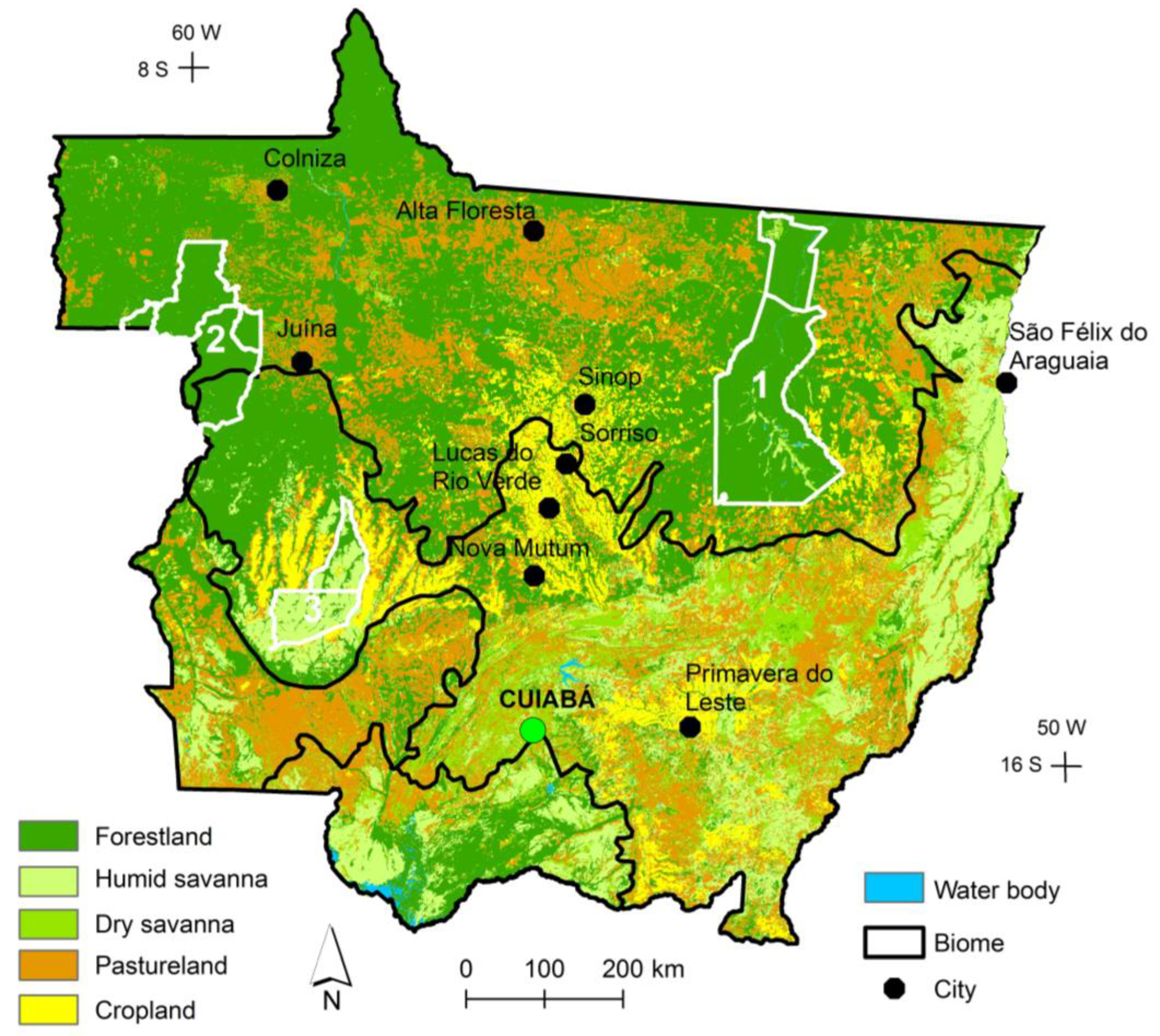
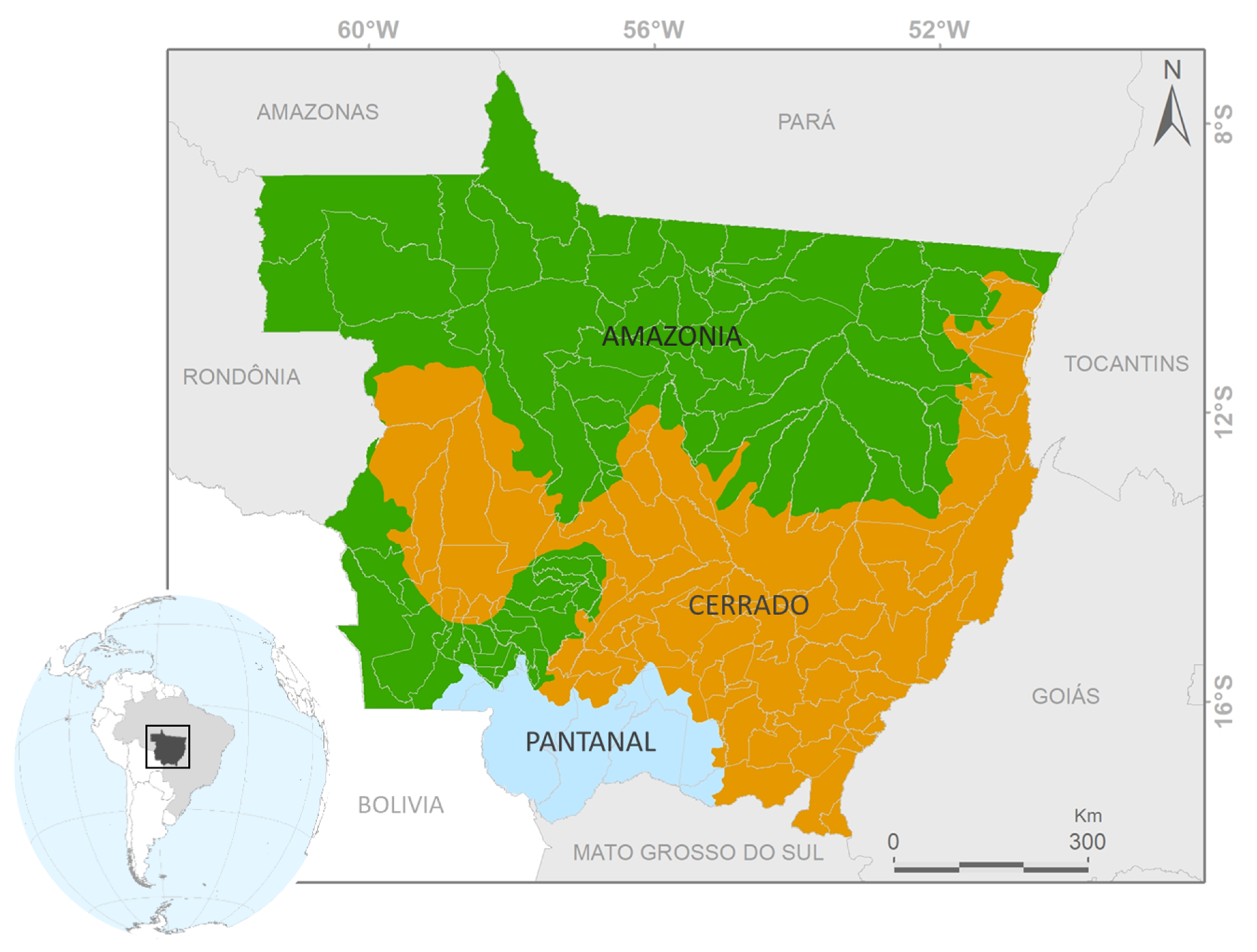
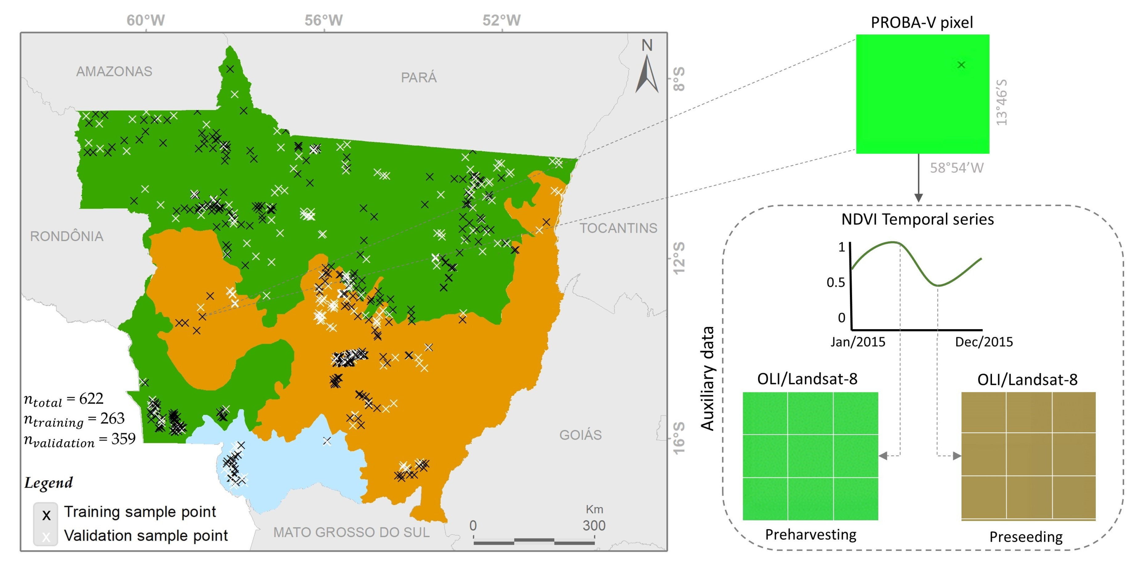
2.1. Study Area
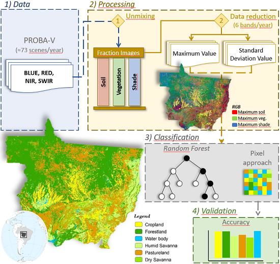
2.2. Datasets
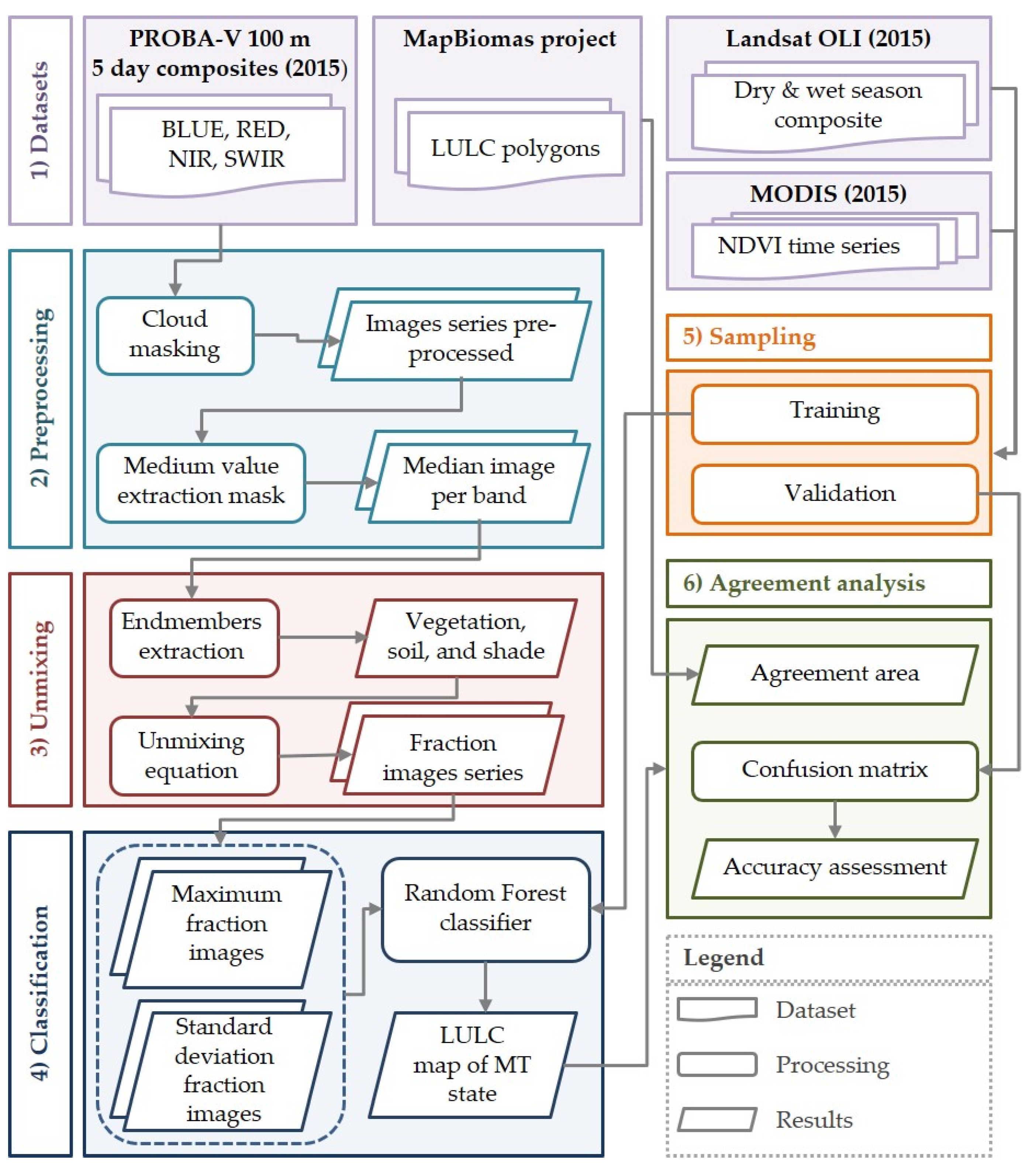
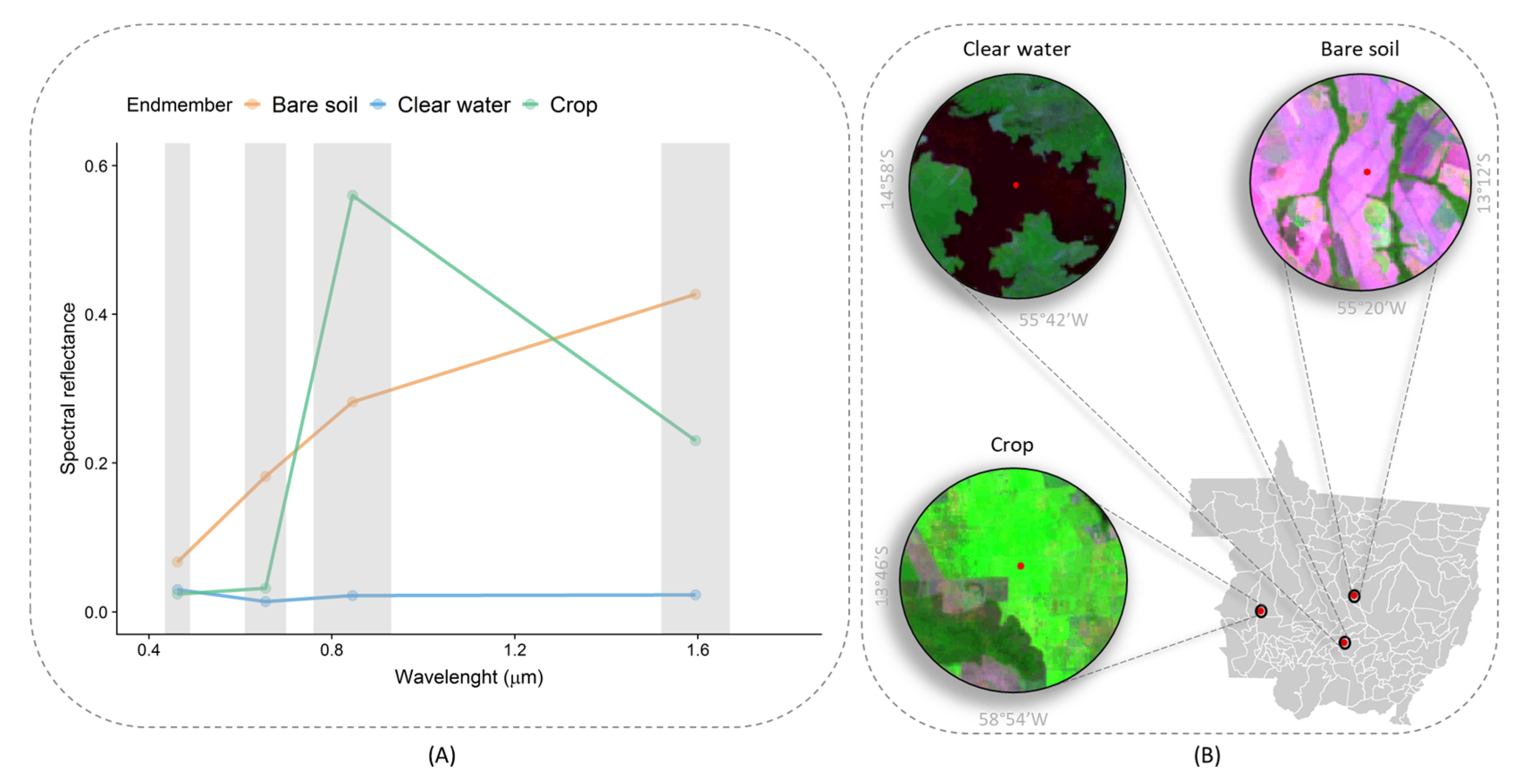
2.3. Data Processing
- Ri = the spectral reflectance in the ith spectral band;
- ri,j = the spectral reflectance of the jth component in the ith spectral band (endmember);
- fi = the proportion of the jth component within the pixel;
- i = 1, p (number of spectral bands used);
- j = 1, m (number of considered components); and
- εi = the residual for the ith spectral band.
2.4. LULC Description
2.5. Sampling Design and Classification
3. Results
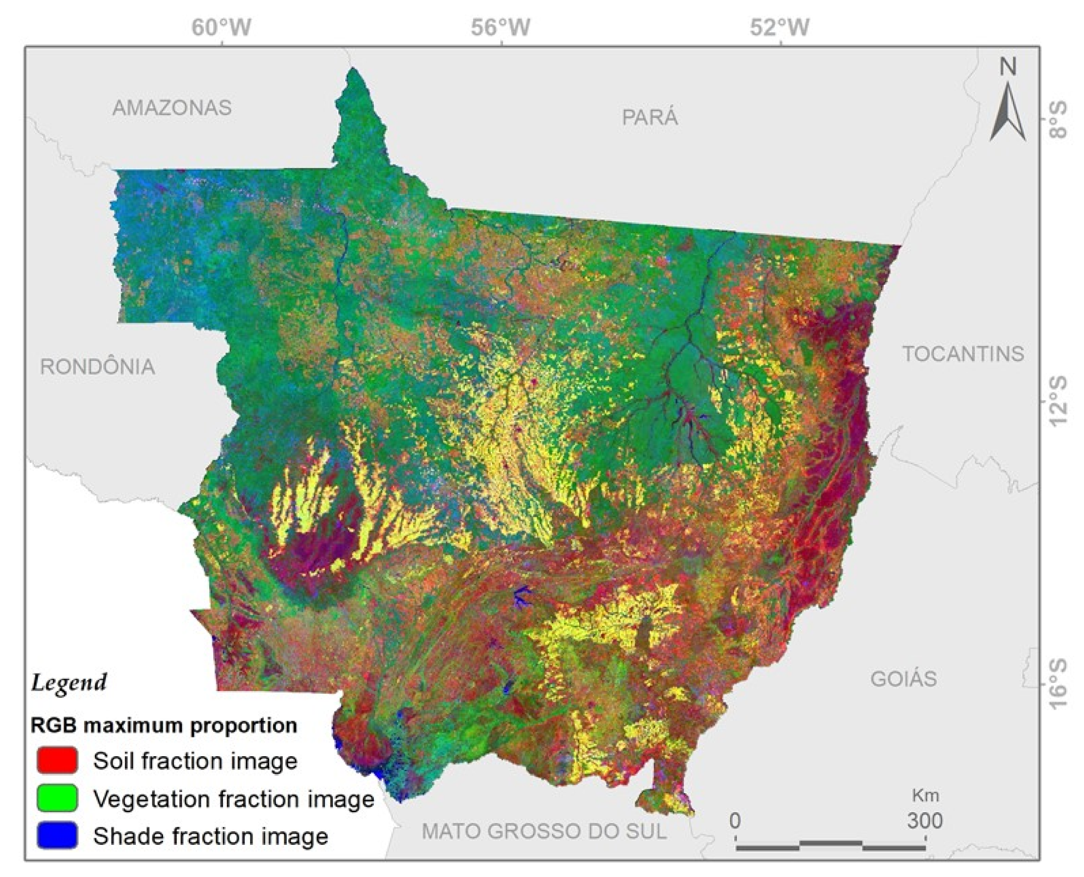
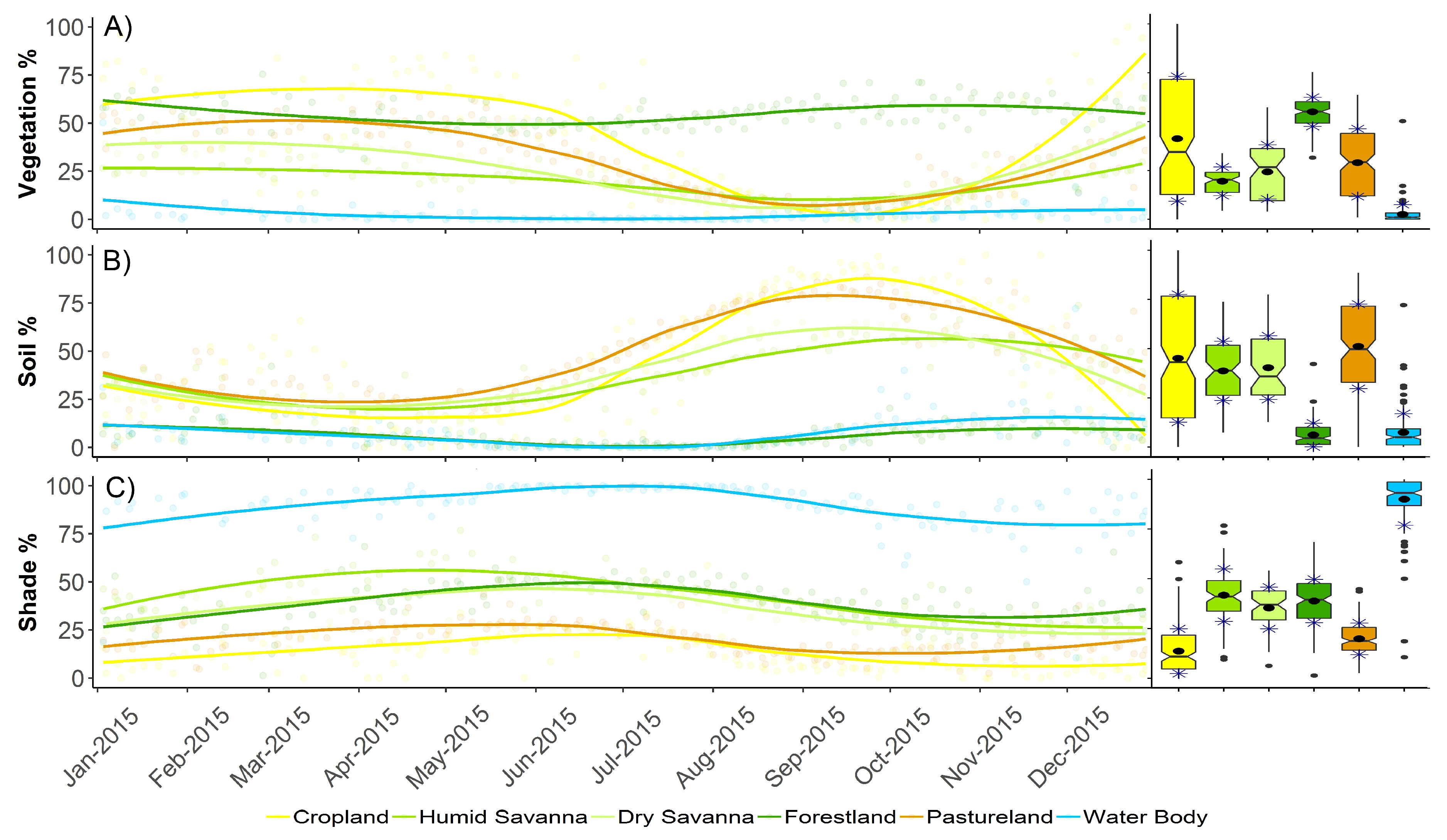
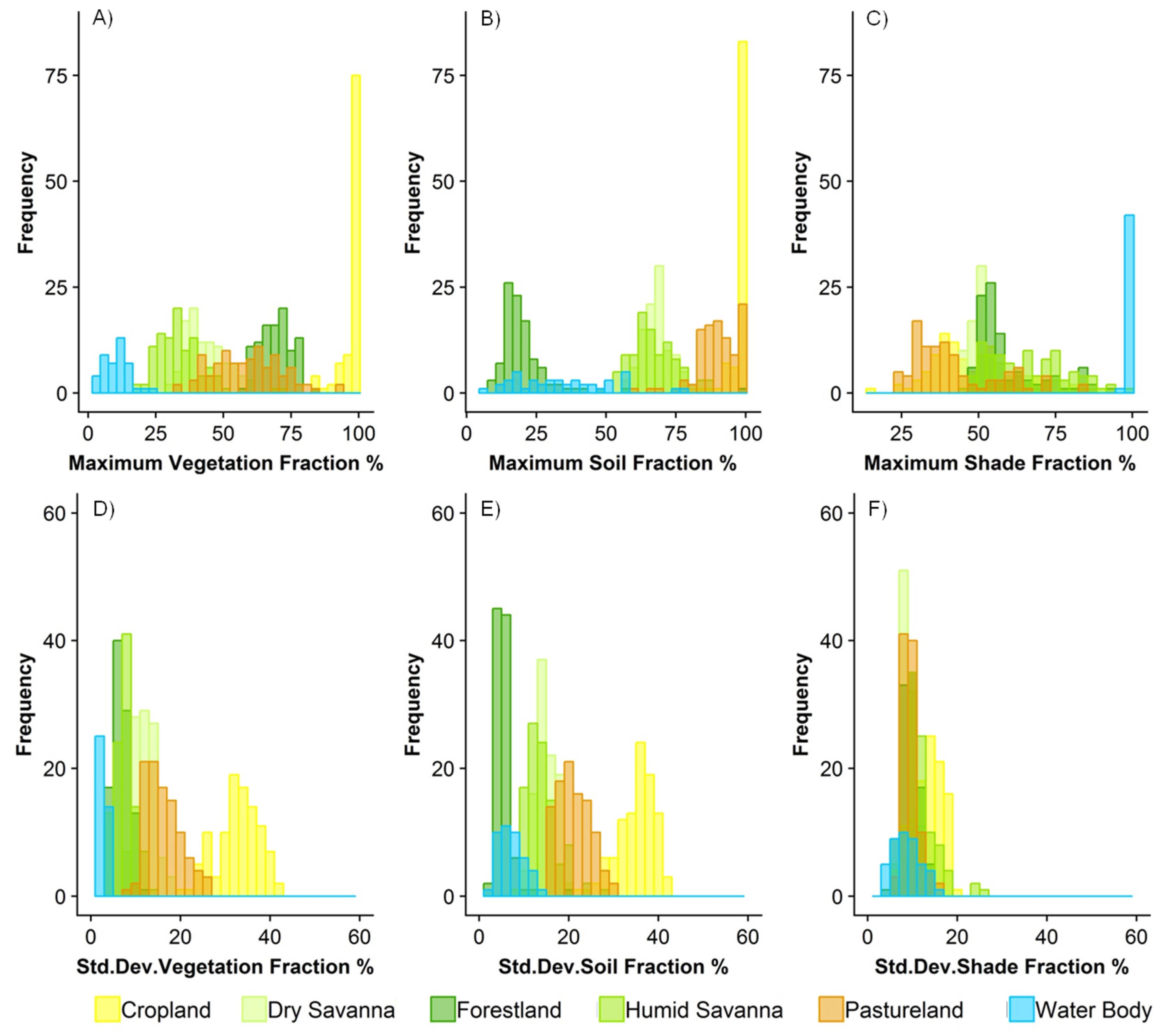
3.1. Maximum and Standard Deviation Fractions of Vegetation, Soil, and Shade
3.2. LULC Map
3.3. Accuracy
4. Discussion
4.1. Classification Performance and Uncertainties
4.2. Novel Approach
4.3. Perspective
5. Conclusions
Author Contributions
Funding
Conflicts of Interest
References
- INPE, National Institute for Space Research. Monitoramento da Floresta Amazônica Brasileira por Satélite/PRODES. 2018. Available online: http://www.obt.inpe.br/OBT/assuntos/programas/amazonia/prodes (accessed on 30 April 2019).
- Mendes, F.S.; Baron, D.; Gerold, G.; Liesenberg, V.; Erasmi, S. Optical and SAR remote sensing synergism for mapping vegetation types in the endangered Cerrado/Amazon ecotone of Nova Mutum—Mato Grosso. Remote Sens. 2019, 11, 1161. [Google Scholar] [CrossRef] [Green Version]
- Klink, C.A.; Moreira, A.G. Past and Current Human Occupation, and Land Use. In The Cerrados of Brazil: Ecology and Natural History of a Neotropical Savanna, 1st ed.; Oliveira, P.S., Marquis, R.J., Eds.; Columbia University Press: New York, NY, USA, 2002; pp. 69–88. [Google Scholar]
- Gollnow, F.; Hissa, L.B.V.; Rufin, P.; Lakes, T. Property-level direct and indirect deforestation for soybean production in the Amazon region of Mato Grosso, Brazil. Land Use Policy 2018, 78, 377–385. [Google Scholar] [CrossRef]
- Parente, L.; Mesquita, V.; Miziara, F.; Baumann, L.; Ferreira, L. Assessing the pasturelands and livestock dynamics in Brazil, from 1985 to 2017: A novel approach based on high spatial resolution imagery and Google Earth Engine cloud computing. Remote Sens. Environ. 2019, 232, 111301. [Google Scholar] [CrossRef]
- Sano, E.E.; Rosa, R.; Brito, J.L.S.; Ferreira, L.G. Land cover mapping of the tropical savanna region in Brazil. Environ. Monit. Assess. 2010, 166, 113–124. [Google Scholar] [CrossRef]
- Lapola, D.M.; Martinelli, L.A.; Peres, C.A.; Ometto, J.P.H.B.; Ferreira, M.E.; Nobre, C.A.; Aguiar, A.P.D.; Bustamante, M.M.C.; Cardoso, M.F.; Costa, M.H.; et al. Pervasive transition of the Brazilian land-use system. Nat. Clim. Chang. 2014, 4, 27–35. [Google Scholar] [CrossRef] [Green Version]
- Kirby, K.R.; Laurance, W.F.; Albernaz, A.K.; Schroth, G.; Fearnside, P.M.; Bergen, S.; Venticinque, E.M.; Costa, C. The future of deforestation in the Brazilian Amazon. Futures 2006, 38, 432–453. [Google Scholar] [CrossRef] [Green Version]
- Laurance, W.F.; Sayer, J.; Cassman, K.G. Agricultural expansion and its impacts on tropical nature. Trends Ecol. Evol. 2014, 29, 107–116. [Google Scholar] [CrossRef] [PubMed]
- Achard, F.; Brown, S.; De Fries, R.; Grassi, G.; Herold, M.; Mollicone, D.; Pandey, D.; Souza, C., Jr. Reducing greenhouse gas emissions from deforestation and degradation in developing countries. In A Sourcebook of Methods and Procedures for Monitoring, Measuring and Reporting; GOFC-GOLD Report version COP14-2; GOFC-GOLD Project Office, Natural Resources Canada: Alberta, Canada, 2009; 185p. [Google Scholar]
- Aragão, L.E.O.C.; Anderson, L.O.; Fonseca, M.G.; Rosan, T.M.; Vedovato, L.B.; Wagner, F.H.; Silva, C.V.J.; Junior, C.H.L.S.; Arai, E.; Aguiar, A.P.; et al. 21st Century drought-related fires counteract the decline of Amazon deforestation carbon emissions. Nat. Commun. 2018, 9, 536. [Google Scholar] [CrossRef]
- Morris, R.J. Anthropogenic impacts on tropical forest biodiversity: A network structure and ecosystem functioning perspective. Philos. Tran. R. Soc. B 2010, 365, 3709–3718. [Google Scholar] [CrossRef] [Green Version]
- Barlow, J.; Lennox, G.D.; Ferreira, J.; Berenguer, E.; Lees, A.C.; Nally, R.M.; Thomson, J.R.; Ferraz, S.F.d.; Louzada, J.; Oliveira, V.H.F.; et al. Anthropogenic disturbance in tropical forests can double biodiversity loss from deforestation. Nature 2016, 535, 144–147. [Google Scholar] [CrossRef] [Green Version]
- Chen, J.; Chen, J.; Liao, A.; Cao, X.; Chen, L.; Chen, X.; He, C.; Han, G.; Peng, S.; Lu, M.; et al. Global land cover mapping at 30 m resolution: A POK-based operational approach. ISPRS J. Photogramm. Remote Sens. 2015, 103, 7–27. [Google Scholar] [CrossRef] [Green Version]
- Hansen, M.C.; Potapov, P.V.; Moore, R.; Hancher, M.; Turubanova, S.A.; Tyukavina, A.; Thau, D.; Stehman, S.V.; Goetz, S.J.; Loveland, T.R.; et al. High-resolution global maps of 21st-century forest cover change. Science 2013, 342, 850–853. [Google Scholar] [CrossRef] [PubMed] [Green Version]
- MapBiomas. MapBiomas v. 3.1. Available online: http://mapbiomas.org/# (accessed on 30 April 2019).
- Parente, L.; Ferreira, L.; Faria, A.; Nogueira, S.; Araújo, F.; Teixeira, L.; Hagen, S. Monitoring the Brazilian pasturelands: A new mapping approach based on the Landsat-8 spectral and temporal domains. Int. J. Appl. Earth Obs. Geoinf. 2017, 62, 135–143. [Google Scholar] [CrossRef]
- Sano, E.E.; Rodrigues, A.A.; Martins, E.S.; Bettiol, G.M.; Bustamante, M.M.C.; Bezerra, A.S.; Couto, A.F., Jr.; Vasconcelos, V.; Schüler, J.; Bolfe, E.L. Cerrado ecoregions: A spatial framework to assess and prioritize Brazilian savanna environmental diversity for conservation. J. Environ. Manag. 2019, 232, 818–828. [Google Scholar] [CrossRef]
- Bendini, H.N.; Fonseca, L.M.G.; Körting, T.S.; Marujo, R.F.B.; Sanches, I.D.; Arcanjo, J.S. Assessment of a multi-sensor approach for noise removal on Landsat-8 OLI time series using CBERS-4 MUX data to improve crop classification based on phenological features. Proc. Brazilian Symp. Geoinform. 2016, 240–251. [Google Scholar]
- Justice, C.O.; Townshend, J.R.G.; Vermote, E.F.; Masuoka, E.; Wolfe, R.E.; Saleous, N.; Roy, D.P.; Morisette, J.T. An overview of MODIS land data processing and product status. Remote Sens. Environ. 2002, 83, 3–15. [Google Scholar] [CrossRef]
- Rast, M.; Bézy, J.; Bruzzi, S. The ESA medium resolution imaging spectroradiometer MERIS: A review of the instrument and its mission. Int. J. Remote Sens. 1999, 20, 1681–1702. [Google Scholar] [CrossRef]
- Dierckx, W.; Sterckx, S.; Benhadj, I.; Livens, S.; Duhoux, G.; van Achteren, T.; Francois, M.; Mellab, K.; Saint, G. PROBA-V mission for global vegetation monitoring: Standard products and image quality. Int. J. Remote Sens. 2014, 35, 2589–2614. [Google Scholar] [CrossRef]
- Bendini, H.N.; Garcia Fonseca, L.M.; Schwieder, M.; Sehn Körting, T.; Rufin, P.; Sanches, I.D.; Leitão, P.J.; Hostert, P. Detailed agricultural land classification in the Brazilian cerrado based on phenological information from dense satellite image time series. Int. J. Appl. Earth Obs. Geoinf. 2019, 82, 101872. [Google Scholar] [CrossRef]
- Roy, D.P.; Huang, H.; Boschetti, L.; Giglio, L.; Yan, L.; Zhang, H.H.; Li, Z. Landsat-8 and Sentinel-2 burned area mapping—A combined sensor multi-temporal change detection approach. Remote Sens. Environ. 2019, 231, 111254. [Google Scholar] [CrossRef]
- Lu, D.; Moran, E.; Batistella, M. Linear mixture model applied to Amazonian vegetation classification. Remote Sens. Environ. 2003, 87, 456–469. [Google Scholar] [CrossRef] [Green Version]
- Somers, B.; Asner, G.P.; Tits, L.; Coppin, P. Endmember variability in spectral mixture analysis: A review. Remote Sens. Environ. 2011, 115, 1603–1616. [Google Scholar] [CrossRef]
- Shimabukuro, Y.E.; Smith, J.A. The least-squares mixing models to generate fraction images derived from remote sensing multispectral data. IEEE Trans. Geosci. Remote Sens. 1991, 29, 16–20. [Google Scholar] [CrossRef]
- Quintano, C.; Fernández-Manso, A.; Shimabukuro, Y.E.; Pereira, G. Spectral unmixing. In. J. Remote Sens. 2012, 33, 5307–5340. [Google Scholar] [CrossRef]
- Haertel, V.; Shimabukuro, Y.E. Spectral linear mixing model in low spatial resolution image data. IEEE Trans. Geosci. Remote Sens. 2005, 43, 2555–2562. [Google Scholar] [CrossRef]
- Anderson, L.O.; Aragão, L.E.O.C.; Shimabukuro, Y.E.; Almeida, S.; Huete, A. Fraction images for monitoring intra-annual phenology of different vegetation physiognomies in Amazonia. Int. J. Remote Sens. 2011, 32, 387–408. [Google Scholar] [CrossRef]
- Ferreira, M.E.; Ferreira, L.G.; Sano, E.E.; Shimabukuro, Y.E. Spectral linear mixture modelling approaches for land cover mapping of tropical savanna areas in Brazil. Int. J. Remote Sens. 2007, 28, 413–429. [Google Scholar] [CrossRef]
- Adami, M.; Bernardes, S.; Arai, E.; Freitas, R.M.; Shimabukuro, Y.E.; Espírito-Santo, F.D.B.; Rudorff, B.F.T.; Anderson, L.O. Seasonality of vegetation types of South America depicted by moderate resolution imaging spectroradiometer (MODIS) time series. Int. J. Appl. Earth Obs. Geoinf. 2018, 69, 148–163. [Google Scholar] [CrossRef] [Green Version]
- Shimabukuro, Y.E.; Arai, E.; Duarte, V.; Jorge, A.; Santos, E.G.; Gasparini, K.A.C.; Dutra, A.C. Monitoring deforestation and forest degradation using multi-temporal fraction images derived from Landsat sensor data in the Brazilian Amazon. Int. J. Remote Sens. 2019, 40, 5475–5496. [Google Scholar] [CrossRef]
- Arvor, D.; Jonathan, M.; Meirelles, M.S.P.; Dubreuil, V.; Durieux, L. Classification of MODIS EVI time series for crop mapping in the State of Mato Grosso, Brazil. Int. J. Remote Sens. 2011, 32, 7847–7871. [Google Scholar] [CrossRef]
- Instituto Brasileiro de Geografia e Estatística (IBGE). Mapa de Biomas e de Vegetação; IBGE: Rio de Janeiro, Brazil, 2004. Available online: https://ww2.ibge.gov.br/home/presidencia/noticias/21052004biomashtml.shtm (accessed on 29 April 2019).
- Cohn, A.S.; Gil, J.; Berger, T.; Pellegrina, H.; Toledo, C. Patterns and processes of pasture to crop conversion in Brazil: Evidence from Mato Grosso State. Land Use Policy 2016, 55, 108–120. [Google Scholar] [CrossRef]
- Koltunov, A.; Ustin, S.L.; Asner, G.P.; Fung, I. Selective logging changes forest phenology in the Brazilian Amazon: Evidence from MODIS image time series analysis. Remote Sens. Environ. 2009, 113, 2431–2440. [Google Scholar] [CrossRef]
- Grecchi, R.C.; Beuchle, R.; Shimabukuro, Y.E.; Aragão, L.E.O.C.; Arai, E.; Simonetti, D.; Achard, F. An integrated remote sensing and GIS approach for monitoring areas affected by selective logging: A case study in northern Mato Grosso, Brazilian Amazon. Int. J. Appl. Earth Obs. Geoinf. 2017, 61, 70–80. [Google Scholar] [CrossRef]
- Francois, M.; Santandrea, S.; Mellab, K.; Vrancken, D.; Versluys, J. The PROBA-V mission: The space segment. Int. J. Remote Sens. 2014, 35, 2548–2564. [Google Scholar] [CrossRef]
- Wolters, E.; Dierckx, W.; Dries, J.; Swinnen, E. PROBA-V Products User Manual v3.01. VITO. 2018. Available online: http://proba-v.vgt.vito.be/sites/proba-v.vgt.vito.be/files/products_user_manual.pdf (accessed on 30 April 2019).
- Gorelick, N.; Hancher, M.; Dixon, M.; Ilyushchenko, S.; Thau, D.; Moore, R. Google Earth Engine: Planetary-scale geospatial analysis for everyone. Remote Sens. Environ. 2017, 202, 18–27. [Google Scholar] [CrossRef]
- Instituto Brasileiro de Geografia e Estatística (IBGE). Censo Agropecuário; IBGE: Rio de Janeiro, Brzail, 2017. Available online: https://www.ibge.gov.br/estatisticas-novoportal/economicas/agricultura-e-pecuaria/21814-2017-censo-agropecuario.html?edicao=21858&t=sobre (accessed on 12 November 2019).
- Schwieder, M.; Leitão, P.J.; Bustamante, M.M.C.; Ferreira, L.G.; Rabe, A.; Hostert, P. Mapping Brazilian savanna vegetation gradients with Landsat time series. Int. J. Appl. Earth Obs. Geoinf. 2016, 52, 361–370. [Google Scholar] [CrossRef]
- Roy, E.D.; Richards, P.D.; Martinelli, L.A.; Della Coletta, L.; Lins, S.R.M.; Vazquez, F.F.; Willig, E.; Spera, S.A.; VanWey, L.K.; Porder, S. The phosphorus cost of agricultural intensification in the tropics. Nat. Plants 2016, 2, 16043. [Google Scholar] [CrossRef]
- Ribeiro, J.F.; Walter, B.M.T. As Principais Fitofisionomias do Bioma Cerrado; Sano, S.M., Almeida, S.P., Ribeiro, J.F., Eds.; Ecologia e Flora: Cerrado, Brazil, 2008; pp. 152–212. [Google Scholar]
- Nogueira, E.M.; Nelson, B.W.; Fearnside, P.M.; França, M.B.; Oliveira, Á.C.A. Tree height in Brazil’s ‘arc of deforestation’: Shorter trees in south and southwest Amazonia imply lower biomass. For. Ecol. Manag. 2008, 255, 2963–2972. [Google Scholar] [CrossRef]
- Olofsson, P.; Foody, G.M.; Herold, M.; Stehman, S.V.; Woodcock, C.E.; Wulder, M.A. Good practices for estimating area and assessing accuracy of land change. Remote Sens. Environ. 2014, 148, 42–57. [Google Scholar] [CrossRef]
- Breiman, L. Random Forests. Mach. Learn. 2001, 5–32. [Google Scholar] [CrossRef] [Green Version]
- Dietterich, T.G. An experimental comparison of three methods for constructing ensembles of decision trees: Bagging, boosting, and randomization. Mach. Learn. 2000, 40, 139–157. [Google Scholar] [CrossRef]
- Hudson, W.D.; Ramm, C.W. Correct formulation of the Kappa coefficient of agreement (in remote sensing). Photogramm. Eng. Remote Sens. 1987, 53, 421–422. [Google Scholar]
- Congalton, R.G. Accuracy assessment and validation of remotely sensed and other spatial information. Int. J. Wildl. Fire 2001, 10, 321. [Google Scholar] [CrossRef] [Green Version]
- Simoes, R.; Picoli, M.C.A.; Camara, G.; Maciel, A.; Santos, L.; Andrade, P.R.; Sánchez, A.; Ferreira, K.; Carvalho, A. Land use and cover maps for Mato Grosso State in Brazil from 2001 to 2017. Sci. Data 2020, 7, 1–10. [Google Scholar]
- Fearnside, P.M. Brazil´s Cuiabá-Santarém (BR-163) highway: The environmental cost of paving a soybean corridor through the Amazon. Environ. Manag. 2007, 39, 601–614. [Google Scholar] [CrossRef] [PubMed]
- Pinheiro, T.F.; Escada, M.I.S.; Valeriano, D.M.; Hostert, P.; Gollnow, F.; Muller, H. Forest degradation associated with logging frontier expansion in the Amazon: The BR-163 region in southwestern Pará, Brazil. Earth Interact. 2016, 17, 1–26. [Google Scholar]
- Latrubesse, E.M.; Stevaux, J.C. Geomorphology and environmental aspects of the Araguaia fluvial basin, Brazil. Z. Geomorphol. 2002, 129, 109–127. [Google Scholar]
- Latrubesse, E.M.; Amsler, M.L.; Morais, R.P.; Aquino, S. The geomorphologic response of a large pristine alluvial river to tremendous deforestation in the South American tropics: The case of the Araguaia river. Geomorphol. 2009, 113, 239–252. [Google Scholar] [CrossRef]
- Picoli, M.C.A.; Camara, G.; Sanches, I.; Simões, R.; Carvalho, A.; Maciel, A.; Coutinho, A.; Esquerdo, J.; Antunes, J.; Begotti, R.A.; et al. Big earth observation time series analysis for monitoring Brazilian agriculture. ISPRS J. Photogramm. Remote Sens. 2018, 145, 328–339. [Google Scholar] [CrossRef]
- IBGE. Produção Agrícola Municipal; IBGE: Rio de Janeiro, Brazil, 2018. Available online: https://sidra.ibge.gov.br/pesquisa/pam/tabelas (accessed on 17 June 2019).
- Zalles, V.; Hansen, M.C.; Potapov, P.V.; Stehman, S.V.; Tyukavina, A.; Pickens, A.; Song, X.-P.; Adusei, B.; Okpa, C.; Aguilar, R.; et al. Near doubling of Brazil’s intensive row crop area since 2000. Proc. Natl. Acad. Sci. USA 2019, 116, 428–435. [Google Scholar] [CrossRef] [Green Version]
- Rudorff, B.F.T.; Aguiar, D.A.; Silva, W.F.; Sugawara, L.M.; Adami, M.; Moreira, M.A. Studies on the rapid expansion of sugarcane for ethanol production in São Paulo State (Brazil) using Landsat data. Remote Sens. 2010, 2, 1057–1076. [Google Scholar] [CrossRef] [Green Version]
- Scaramuzza, C.A.M.; Sano, E.E.; Adami, M.; Bolfe, E.L.; Coutinho, A.C.; Esquerdo, J.C.D.M.; Maurano, L.E.P.; Narvaes, I.d.S.; Oliveira Filho, F.J.B.D.; Rosa, R.; et al. Land-use and land-cover mapping of the Brazilian Cerrado based mainly on Landsat-8 satellite images. Rev. Bras. Cartogr. 2017, 69, 1041–1051. [Google Scholar]
- Almeida, C.A.; Coutinho, A.C.; Esquerdo, J.C.D.M.; Adami, M.; Venturieri, A.; Diniz, C.G.; Dessay, N.; Durieux, L.; Gomes, A.R. High spatial resolution land use and land cover mapping of the Brazilian Legal Amazon in 2008 using Landsat-5/TM and MODIS data. Acta Amaz. 2016, 46, 291–302. [Google Scholar] [CrossRef]
- Alvares, C.A.; Stape, J.L.; Sentelhas, P.C.; Moraes, G.; Leonardo, J.; Sparovek, G. Köppen’s climate classification map for Brazil. Meteorol. Z. 2013, 22, 711–728. [Google Scholar] [CrossRef]
- Sterckx, S.; Benhadj, I.; Duhoux, G.; Livens, S.; Dierckx, W.; Goor, E.; Adriaensen, S.; Heyns, W.; van Hoof, K.; Strackx, G.; et al. The PROBA-V mission: Image processing and calibration. Int. J. Remote Sens. 2014, 35, 2565–2588. [Google Scholar] [CrossRef]
- Müller, H.; Rufin, P.; Griffiths, P.; Barros Siqueira, A.J.; Hostert, P. Mining dense Landsat time series for separating cropland and pasture in a heterogeneous Brazilian savanna landscape. Remote Sens. Environ. 2015, 156, 490–499. [Google Scholar] [CrossRef] [Green Version]
- Thorp, K.R.; French, A.N.; Rango, A. Effect of image spatial and spectral characteristics on mapping semi-arid rangeland vegetation using multiple endmember spectral mixture analysis (MESMA). Remote Sens. Environ. 2013, 132, 120–130. [Google Scholar] [CrossRef]
- Yang, J.; Weisberg, P.J.; Bristow, N.A. Landsat remote sensing approaches for monitoring long-term tree cover dynamics in semi-arid woodlands: Comparison of vegetation indices and spectral mixture analysis. Remote Sens. Environ. 2012, 119, 62–71. [Google Scholar] [CrossRef]
- Souza, C.M.; Roberts, D.A.; Cochrane, M.A. Combining spectral and spatial information to map canopy damage from selective logging and forest fires. Remote Sens. Environ. 2005, 98, 329–343. [Google Scholar] [CrossRef]
- Bullock, E.L.; Woodcock, C.E.; Souza, C.; Olofsson, P. Satellite-based estimates reveal widespread forest degradation in the Amazon. Glob. Chang. Biol. 2020, 26, 2956–2969. [Google Scholar] [CrossRef]
- Naidoo, L.; Mathieu, R.; Main, R.; Wessels, K.; Asner, G.P. L-band synthetic aperture radar imagery performs better than optical datasets at retrieving woody fractional cover in deciduous, dry savannahs. Int. J. Appl. Earth Obs. Geoinf. 2016, 52, 54–64. [Google Scholar] [CrossRef]
- Lee, J.; Cardille, J.A.; Coe, M.T. Agricultural expansion in Mato Grosso from 1986–2000: A Bayesian time series approach to tracking past land cover change. Remote Sens. 2020, 12, 688. [Google Scholar] [CrossRef] [Green Version]
- Fortin, J.A.; Cardille, J.A.; Perez, E. Multi-sensor detection of forest-cover change across 45 years in Mato Grosso, Brazil. Remote Sens. Environ. 2020, 238, 111266. [Google Scholar] [CrossRef]
| 1 | Available in www.satveg.cnptia.embrapa.br. Accessed on 30 June 2019. |


| This Study | MapBiomas Project |
|---|---|
| Croplands | Annual and perennial crop and semiperennial crop |
| Forestland | Forest formation and forest plantation |
| Water bodies | River, lake and ocean |
| Humid savanna | Mangrove, wetland, and other nonforest natural formation |
| Pastureland | Grassland formation, pasture, and mosaic of agriculture and pasture |
| Dry savanna | Savanna formation |
| LULC Class | Amazonia | Cerrado | Pantanal | Subtotal |
|---|---|---|---|---|
| Croplands | 14,178 | 25,111 | 175 | 39,464 |
| Forestland | 310,353 | 89,329 | 22,272 | 421,954 |
| Water bodies | 955 | 773 | 1701 | 3429 |
| Humid savanna | 17,406 | 93,790 | 20,679 | 131,875 |
| Pastureland | 124,133 | 92,772 | 11,304 | 228,208 |
| Dry savanna | 18,584 | 50,735 | 8016 | 77,336 |
| Subtotal | 485,609 | 352,510 | 64,147 | 902,266 |
| Reference/ Classified | Cropland (67/84) | Forest-Land (72/56) | Water Body (29/14) | Humid Savanna (64/36) | Pasture-Land (63/37) | Dry Savanna (64/36) | Total (263/359) | UA |
|---|---|---|---|---|---|---|---|---|
| Cropland | 76 | 0 | 0 | 0 | 8 | 0 | 84 | 90 |
| Forestland | 0 | 55 | 0 | 0 | 1 | 0 | 56 | 98 |
| Water Body | 0 | 0 | 14 | 0 | 0 | 0 | 14 | 100 |
| Humid Savanna | 0 | 0 | 0 | 31 | 0 | 5 | 36 | 86 |
| Pastureland | 0 | 0 | 0 | 0 | 35 | 2 | 37 | 95 |
| Dry Savanna | 0 | 0 | 0 | 3 | 1 | 32 | 36 | 89 |
| Total | 76 | 55 | 14 | 34 | 45 | 39 | 263 | |
| PA | 100 | 100 | 100 | 91 | 78 | 82 | 92 |
| Reference/ Classified | Cropland | Forestland | Water Body | Humid Savanna | Pastureland | Dry Savanna | Total | UA |
|---|---|---|---|---|---|---|---|---|
| Cropland | 83 | 0 | 0 | 1 | 0 | 0 | 84 | 99 |
| Forestland | 0 | 56 | 0 | 0 | 0 | 0 | 56 | 100 |
| Water Body | 0 | 0 | 14 | 0 | 0 | 0 | 14 | 100 |
| Humid Savanna | 0 | 0 | 0 | 19 | 2 | 15 | 36 | 53 |
| Pastureland | 0 | 0 | 0 | 1 | 36 | 0 | 37 | 97 |
| Dry Savanna | 0 | 0 | 0 | 12 | 1 | 23 | 36 | 64 |
| Total | 83 | 56 | 14 | 33 | 39 | 38 | 263 | |
| PA | 100 | 100 | 100 | 58 | 92 | 61 | 88 |
| Classes | This study (km2) | MapBiomas (km2) | Difference |
|---|---|---|---|
| Cropland | 39,464 | 52,219 | −32% |
| Forestland | 421,954 | 432,923 | −3% |
| Water Body | 3429 | 17,711 | −416% |
| Dry Savanna | 131,875 | 97,944 | 26% |
| Pastureland | 228,208 | 231,189 | −1% |
| Humid Savanna | 77,336 | 68,962 | 11% |
| Total | 902,266 | 900,947 |
© 2020 by the authors. Licensee MDPI, Basel, Switzerland. This article is an open access article distributed under the terms and conditions of the Creative Commons Attribution (CC BY) license (http://creativecommons.org/licenses/by/4.0/).
Share and Cite
Godinho Cassol, H.L.; Arai, E.; Eyji Sano, E.; Dutra, A.C.; Hoffmann, T.B.; Shimabukuro, Y.E. Maximum Fraction Images Derived from Year-Based Project for On-Board Autonomy-Vegetation (PROBA-V) Data for the Rapid Assessment of Land Use and Land Cover Areas in Mato Grosso State, Brazil. Land 2020, 9, 139. https://doi.org/10.3390/land9050139
Godinho Cassol HL, Arai E, Eyji Sano E, Dutra AC, Hoffmann TB, Shimabukuro YE. Maximum Fraction Images Derived from Year-Based Project for On-Board Autonomy-Vegetation (PROBA-V) Data for the Rapid Assessment of Land Use and Land Cover Areas in Mato Grosso State, Brazil. Land. 2020; 9(5):139. https://doi.org/10.3390/land9050139
Chicago/Turabian StyleGodinho Cassol, Henrique Luis, Egidio Arai, Edson Eyji Sano, Andeise Cerqueira Dutra, Tânia Beatriz Hoffmann, and Yosio Edemir Shimabukuro. 2020. "Maximum Fraction Images Derived from Year-Based Project for On-Board Autonomy-Vegetation (PROBA-V) Data for the Rapid Assessment of Land Use and Land Cover Areas in Mato Grosso State, Brazil" Land 9, no. 5: 139. https://doi.org/10.3390/land9050139