Article

Is There an Equivalence between Measures of Landscape Structural and Functional Connectivity for Plants in Conservation Assessments of the Cerrado?

by
Thais Martins Issii
1,
Erico Fernando Lopes Pereira-Silva
2,
Carlos Tomás López de Pablo
3,
Rozely Ferreira dos Santos
2 and
Elisa Hardt
1,*
1
Department of Environmental Sciences, Universidade Federal de São Paulo, UNIFESP, São Paulo 09913-030, Brazil
2
Department of Ecology, Universidade de São Paulo, USP, São Paulo 05508-090, Brazil
3
Department of Biodiversity, Ecology and Evolution, Universidad Complutense de Madrid, UCM, 28040 Madrid, Spain
*
Author to whom correspondence should be addressed.
Land 2020, 9(11), 459; https://doi.org/10.3390/land9110459
Submission received: 10 October 2020 / Revised: 12 November 2020 / Accepted: 16 November 2020 / Published: 18 November 2020
(This article belongs to the Special Issue Landscape Transformation and Changes in Land Use Intensity)

Abstract

:
Landscape connectivity can be assessed based on the physical connection (structural connectivity) or the maintenance of flow among habitats depending on the species (functional connectivity). The lack of empirical data on the dispersal capacity of species can lead to the use of simple structural measures. Comparisons between these approaches can improve decision-making processes for the conservation or restoration of habitats in fragmented landscapes, such as the Cerrado biome. This study aimed to understand the correspondence between the measures of landscape structural and functional connectivity for Cerrado plants. Three landscapes with cerradão patches in a pasture matrix were selected for the application of these metrics based on the functional connectivity of four profiles of plant dispersal capacity. The results showed divergent interpretations between the measures of landscape structural and functional connectivity, indicating that the assessment of biodiversity conservation and landscape connectivity is dependent on the set of metrics chosen. Structurally, the studied landscapes had the same number of cerradão patches but varied in optimal resource availability, isolation, heterogeneity, and aggregation. Functional connectivity was low for all profiles (based on the integral index of connectivity—IIC) and null for species with a low dispersal capacity (based on the connectance index—CONNECT), indicating that species with a medium- to long-distance dispersal capacity may be less affected by the history of losses and fragmentation of the Cerrado in the pasture matrix. The functional connectivity metrics used allowed a more robust analysis and, apparently, better reflected reality, but the lack of empirical data on dispersal capacity and the difficulty in choosing an indicator organism can limit their use in the management and planning of conservation and restoration areas.

1. Introduction

Landscape connectivity is considered an efficient indirect measure of biodiversity conservation, useful for understanding the effects of environmental changes on organism dispersal [1,2]. Ideally, connectivity measures should include the physical continuity of the environment (structural connectivity) and the peculiarities of movement behavior and dispersal intrinsic to the species (functional connectivity), which vary depending on the morphophysiological patterns and relationships of the species with different types of environment [3,4]. Most studies on functional connectivity have focused on fauna dispersal capacity [5,6,7,8,9]. Some studies have examined plant functional connectivity based on propagules [10,11,12,13], but the current knowledge available is still not enough to understand this phenomenon, especially in highly fragmented landscapes [14]. However, the advance of geotechnologies in recent decades has allowed the development of software and computational models capable of easily obtaining several measures of landscape structure that can be potentially indicative of the quantity and quality of the habitat, such as the number, size, shape, and isolation of habitats obtained using Fragstats® [15,16]. New options have also been developed to measure landscape functionality, such as Conefor® [17], which requires empirical data on the dispersal capacity of study species, differentiating connectivity into three types: within a patch, by flow, and by the connections between patches [18].
In this context, as scientific studies are increasingly concerned with obtaining functional data [19], a shift from structural analysis to functional connectivity measurement is expected. In Brazil, the agencies responsible for the conservation planning and management of natural areas already use geographic information tools to map and monitor areas and to help their decision-making, allowing and facilitating the use of structural connectivity measures (e.g., Euclidean nearest-neighbor distance using Fragstats). However, metrics that better reflect reality, such as functional connectivity (e.g., Integral index of connectivity using Conefor), are not routinely used by public agencies, possibly due to the lack of empirical data on the dispersal capacity of local species. This deficiency is significant for the Cerrado, the second largest Brazilian biome [20] and a global biodiversity hotspot. The Cerrado is poorly protected with deforestation rates 2.5 times higher than that of the Amazon [21]. Among the main drivers of deforestation in the Cerrado is the advance of the agricultural frontier and cattle ranching activities, with 70% of cultivated pastures concentrated in this biome [22]. Given this anthropogenic pressure, it is urgent to establish a conservation and restoration plan with effective strategies, such as maintaining the functional connectivity of species in the Cerrado.
Based on the assumption that functional connectivity cannot always be extrapolated from structural connectivity [23], studies that examine whether there is complementarity or divergence between these inferences of connectivity are essential. Therefore, this study aimed to understand the relationship between the measures of landscape structural and functional connectivity for the dispersal of Cerrado plants. Given the theoretical and methodological differences of these measures, this study was premised on the differential contribution of functional connectivity for plants compared to that of the structural measures, providing complementary information to support decisions on habitat conservation and restoration.

2. Materials and Methods

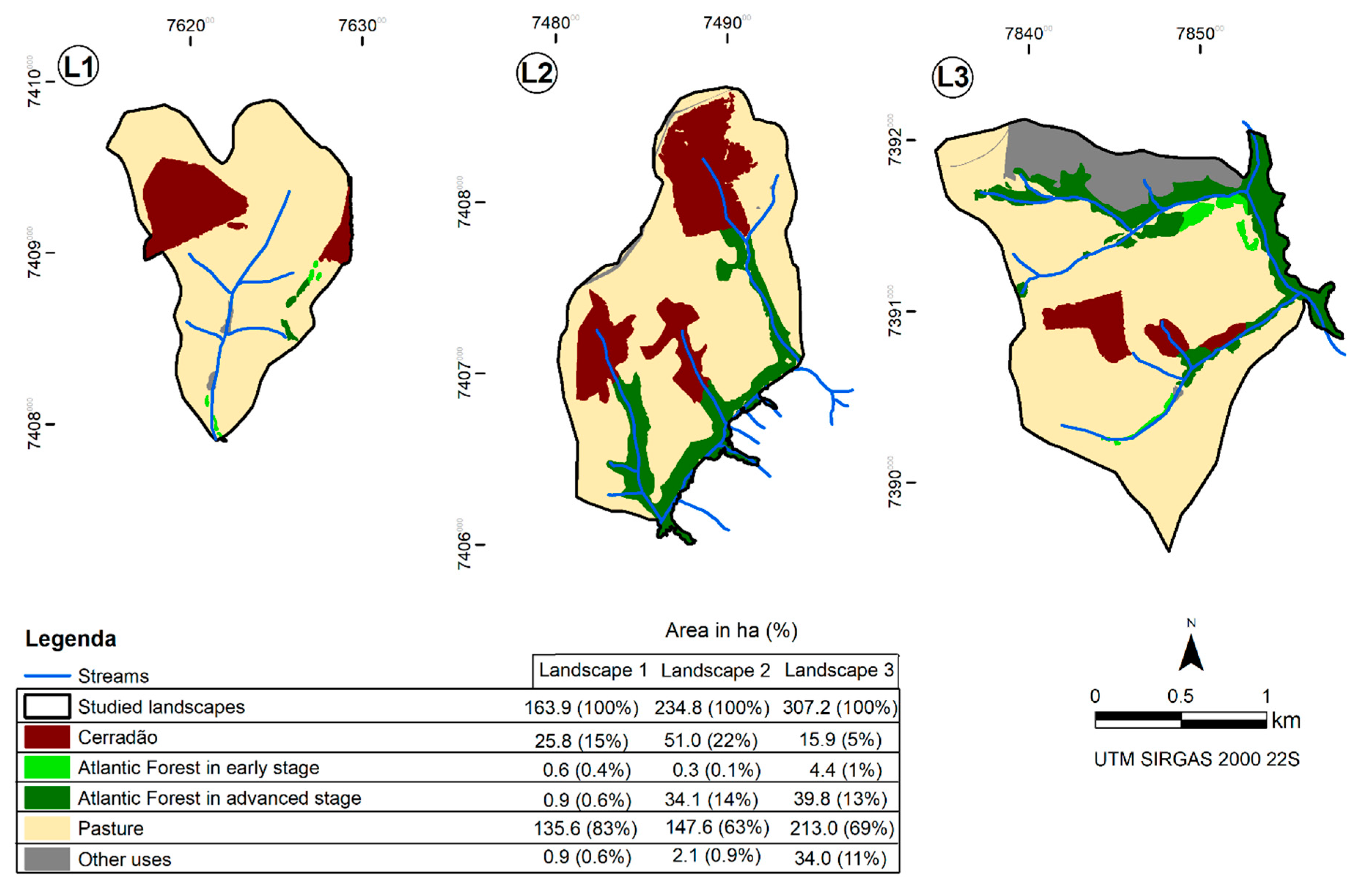
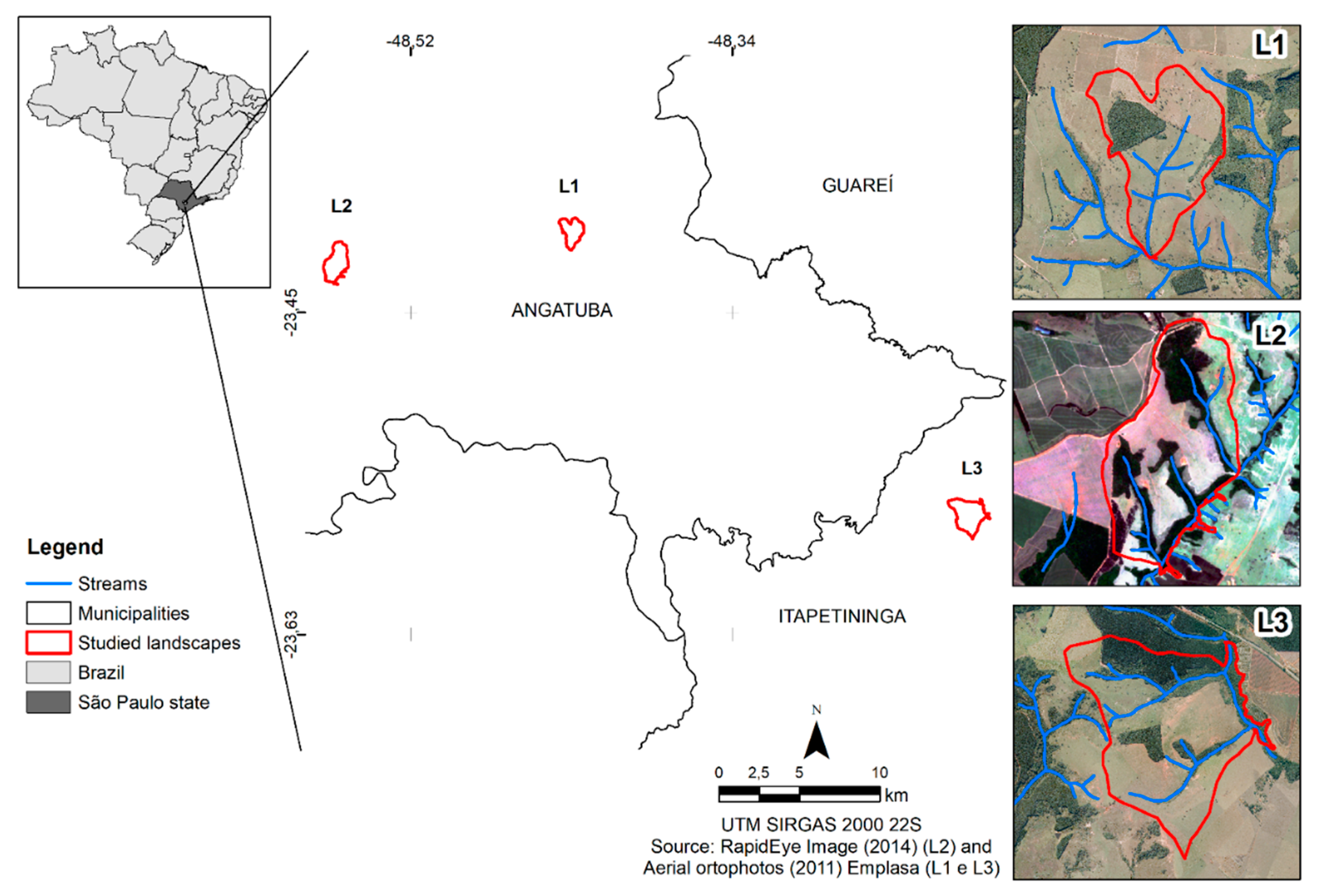
2.1. Selection and Mapping of the Study Area

This study was carried out in the state of São Paulo in three representative landscapes of pasture matrix in an area of the Cerrado domain. In this area, the last remnants of cerradão (CER, a Cerrado forest physiognomy), which are immersed in anthropogenic uses, are mixed with seasonal semideciduous forest, remnants of the Atlantic Forest biome (AF). The size of the fragments (median 9.3, mean 10.3 ± 9.6 ha) in the studied landscapes is characteristic of the Cerrado remnants in the São Paulo state, where for more than a decade, 70.8% of the fragments have had an area of up to 20 ha [24]. The study areas were defined by the limits of the third order basin (the main watercourse drainage resulting from the confluence of two second order rivers). The choice of this geomorphological unit as a scale of analysis is consistent with its ability to reflect the impacts of human activities in the context of local agricultural properties and is usually used as a basic planning unit for the preservation of natural resources and agricultural production [25]. Furthermore, it may influence the dispersal process of the flora affected by landscape characteristics, such as slope and terrain elevation [26,27,28]. Using Google Earth® images and maps of vegetation cover (official forest inventory of 2010) [29], hydrography, and contour lines [30], all the basins in the region that met the following criteria were initially pre-selected: (i) a homogeneous pasture matrix, (ii) a minimum of two CER forest patches, and (iii) a maximum of 10% of other types of land use. After confirming the type of forest (CER or AF) in loco (2018) in the 10 pre-selected landscapes, only three met criteria (ii) (Figure 1). It is important to highlight that there are almost no more remnants of cerradão in pasture matrices in this region. The low number of landscape repetitions is a result of the history of the Cerrado conversion to pasture in the study region and to other types of anthropic exploration in São Paulo state. The loss and fragmentation of the Cerrado in São Paulo accelerated after 1950 with the expansion of agricultural activities to the interior of the State [31]. This loss reached at least 88.5% between 1960 and 2000 [24], and, currently, the coverage of Cerrado occupies less than 1% of São Paulo state, which corresponds to 17% of its original coverage [32]. In Brazil, apart from in the Amazon region, the current policy for the protection of the Cerrado biome requires that 20% of private lands be set aside for conservation [33]. Despite that, in general, Brazil has a history of low environmental law compliance [34,35,36,37], which might help to explain why only three of the pre-selected landscapes met the criteria.
The delimitation in the basins and the creation of the land use and land cover (LULC) maps of the studied landscapes (L1, L2, and L3) were carried out in ArcGIS® version 10.4. The basin boundaries were mapped using topographic maps from the Geographic and Cartographic Institute of the State of São Paulo (IGC—Instituto Geográfico e Cartográfico do Estado de São Paulo) on a 1:10,000 scale, available online on the DataGeo portal [38], coupled with ArcGIS®. The LULC maps were created through visual interpretation performed by only one photo interpreter at a display scale of 1:3000 using aerial photographs from 2011, with a scale of 1:25,000 and 1 m pixel, provided by the São Paulo State Planning Company (EMPLASA—Empresa de Planejamento do Estado de São Paulo). The validation of the mapped LULC categories (CER, AF in early and intermediate–advanced stages, pasture, and other land uses, such as forestry, lakes/ponds, and roads) was carried out after the field surveys and updates of the satellite images (2018) from Google Earth® Pro.

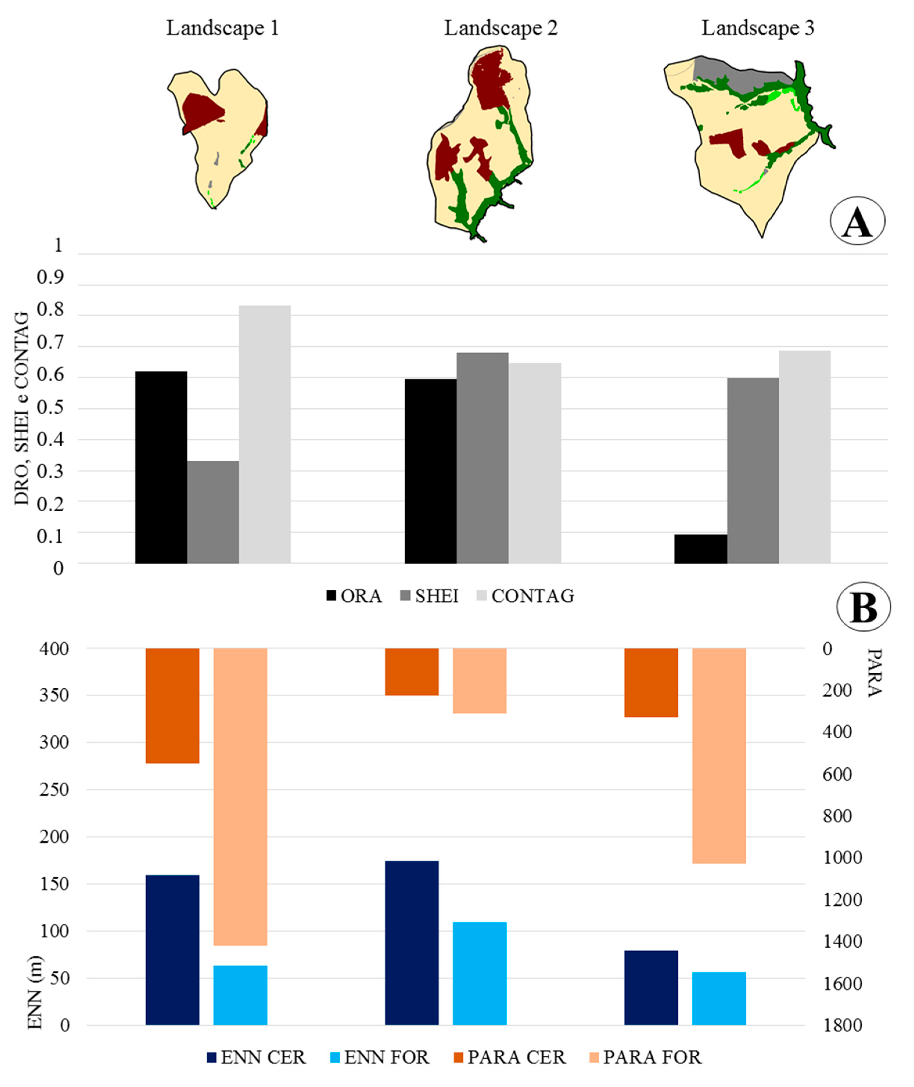
2.2. Measures of Landscape Structure

The analysis of the landscape structure was performed using a set of metrics usually applied in the studies of landscape ecology for biological conservation [35,39,40,41] (Table 1, Equations (1)–(6)). Forest patches were assessed for their Optimal Resource Availability (ORA), calculated in ArcGIS® (extension V-Late) using information on shape (Fsh), their size coefficients (CS), and the physiognomic importance of the forest patches (CF), an adaptation of the literature [39,42] with the inclusion of CF. Weighting CF was performed to enhance the natural habitat of the Cerrado species used in the functional analysis of this study, some of which are exclusive to this Biome. The following values were assigned: (3) for CER patches, (2) for AF at intermediate–advanced stages, and (1) for AF at an early stage. Forest fragmentation was evaluated based on a set of simple and common metrics that represents the main variables of importance for forest conservation and quality using structural measures: number (NP), shape (determined by the Perimeter/Area ratio—PARA), and the isolation (ENN_MN) of patches, all calculated using Fragstats® version 4.2 [15]. With this same software, measurements of landscape heterogeneity and aggregation were also obtained using the Shannon Evenness (SHEI) and Contagion (CONTAG) indexes.
The calculation of these landscape structural measures included: (i) entire forest cover (FOR = CER + AF) and (ii) CER patches. The comparison of these analyses allowed evaluation of the Atlantic Forest contribution in the conservation of the study landscapes, considering its relative importance in maintaining the connectivity of the Cerrado in these pasture matrices.

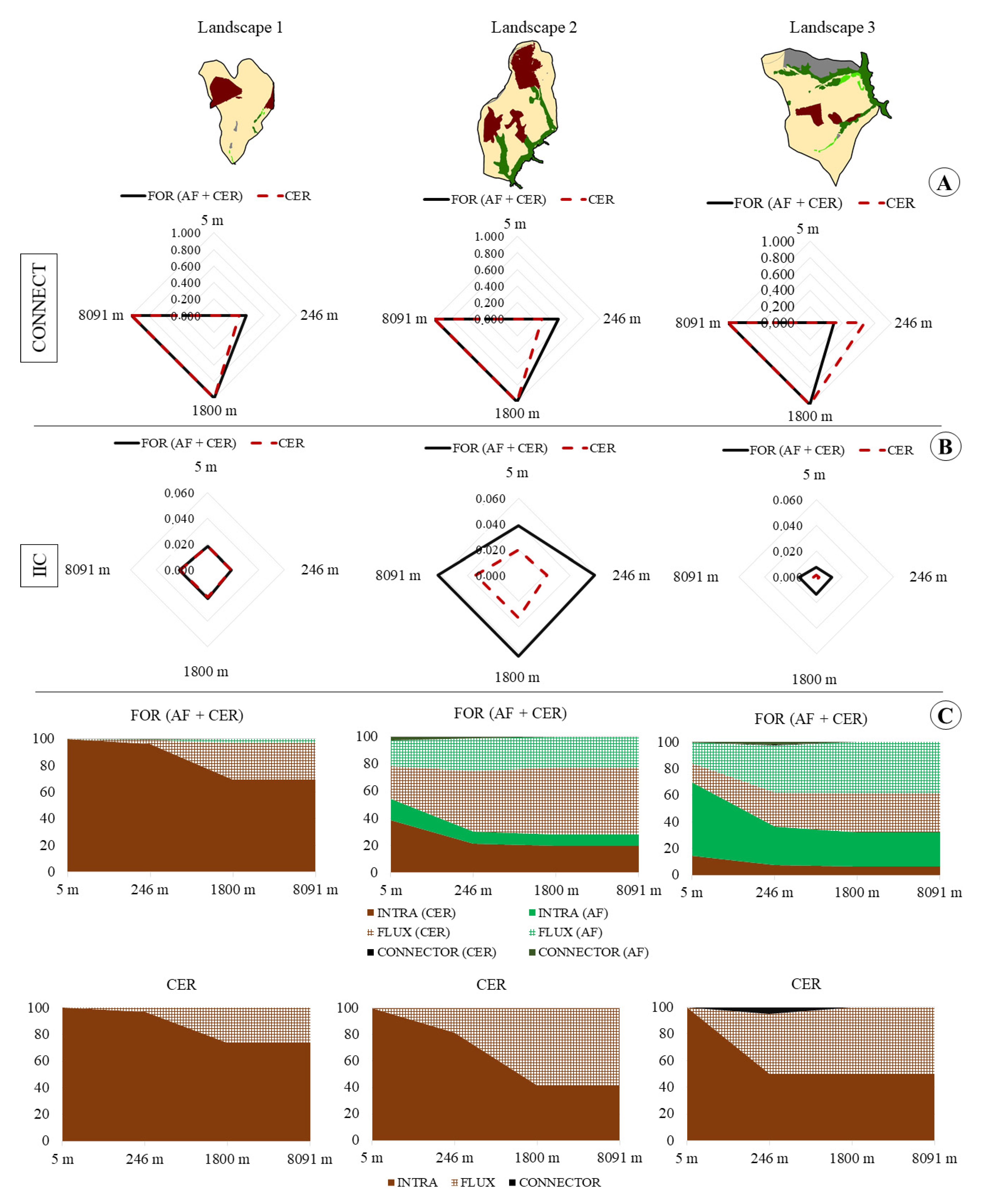
2.3. Measures of Landscape Functional Connectivity

In the functional connectivity estimation, four categories of plant species dispersal distance were considered: short, medium, medium–long, and long. These categories were defined based on secondary data on the dispersal capacity of a set of indicator species (Table 2). The application of these measures indirectly allowed an assessment of the capacity of the study landscapes to promote plant species flow between habitat patches and inferences to be made about the potential for the recolonization of new areas.
Most of the distance values used were based on empirical data on the zoochoric seed dispersal of typical Cerrado species [43,44,45], with a wide geographic distribution in Brazil and occurrences in the state of São Paulo [46] and in the study landscapes. Short dispersal, which potentially also represents propagation by resprouting, was the only category with reference values of dispersal from temperate plant formations [47] due to the lack of distance data for this dispersal category in the Cerrado.
Measures of functional connectivity were obtained from the Connectance Index (CONNECT) and Integral Index Connectivity (IIC), using the Fragstats® and Conefor Sensinode® software version 2.6, respectively [15,48] (Table 1, Equations (7) and (8)). Both measures are a binary model in which functional connections exist (1) or not (0) for a given threshold of dispersal distance, differentiated into the four categories previously described (maximum distances in Table 2).
The methodological difference of the IIC is the graph theory, which represents the landscape as a set of nodes and links [49]. This approach allowed an assessment of the importance of landscape elements to the maintenance of connectivity (dIIC), based on the quality of the habitat patches (intrapatch connectivity), the flow they are capable of providing (flux), and their connections in the landscape (interpatch connectivity) [18]. Based on the sum of the AF and CER patches, their contributions to landscape connectivity maintenance were estimated. In practice, three sets of information were used in the plugin ArcGIS® Conefor inputs: (i) distance threshold (m), based on the maximum dispersal capacity of the species in the four distance profiles considered; (ii) node file, with a quality attribute for each habitat patch, assessed by the product between its cover area (m2) and the coefficient of importance of the forest physiognomy (CF, Table 1); and (iii) connection file, with Euclidean distances between the edges of the habitat patches (m). We have highlighted the use of maximum dispersal distances, rather than the median, in accordance with the application of binary metrics, where the connection exists or does not. Appendix A Figure A1 provides more details about the choice of binary model and shows the same analysis for a probabilistic model (Probability of Connectivity—PC) [50].

3. Results

Landscape 2 (L2) had the highest percentage of total forest cover (FOR2 = 36%) and of cerradão (CER2 = 22%) (Figure 2). Landscapes 1 and 3 (L1 and L3) had similar total values (FOR1 = 16% and FOR3 = 19%), but the percentage of cerradão in L1 was three times that in L3 (CER1 = 15% and CER3 = 5%). Regarding optimal resource availability, L1 and L2 were similar (ORA1 = 0.62; ORA2 = 0.59), while the ORA in L3 was approximately 85% smaller (ORA3 = 0.09) (Figure 3A).
All landscapes had the same number of CER patches (NPCER = 3), but they varied in the quantity of AF patches (NPAF1 = 8; NPAF2 = 2; NPAF3 = 12) (Figure 3B). Most of the L2 and L3 AF patches formed corridors contiguous to CER patches, forming the same fragment of native vegetation (Figure 2). In L2, the FOR and CER had the most regular and uniform shapes (PARAFOR1 = 1419; PARACER1 = 553; PARAFOR2 = 312; PARACER2 = 229; PARAFOR3 = 1029; PARACER3 = 331) (Figure 3B), despite the corridor shape of the AF patches. However, the mean isolation of this landscape was approximately twice that of the others (ENN_MN1 = 62 m; ENN_MN2 = 109 m; ENN_MN3 = 55 m).
Landscape 1 was the most homogeneous and had classes of more aggregated patches (SHEI1 = 0.33 and CONTAG1 = 0.83) (Figure 3A). L2 and L3 had similar diversity and contagion indices, but they were moderately homogeneous and aggregated (SHEI2 = 0.68; SHEI3 = 0.60; CONTAG2 = 0.64 and CONTAG3 = 0.69).
The measure based on CONNECT indicated that the three landscapes had no functional connectivity for short-distance (5 m) dispersal and were 100% connected for medium–long- (1800 m) and long-distance (8091 m) dispersal (Figure 4A). Regarding the mean distance (246 m), functional connectivity was variable—higher in L2 when considering the FOR (CONNECTFOR1 = 38; CONNECTFOR2 = 50; CONNECTFOR3 = 30) and higher in L3 based on the CER (CONNECTCER1 = 33; CONNECTCER2 = 33; CONNECTCER3 = 66).
However, based on the IIC metric, the three landscapes had a low potential for functional connectivity for the plant species evaluated regardless of dispersal profile, as the highest IIC value obtained was 0.063. In all dispersal profiles, L2 represented the best scenario for plant functional connectivity (IICFOR1 = 0.022; IICFOR2 = 0.063; IICFOR3 = 0.014) (Figure 4B). This same pattern was observed for the CER (IICCER1 = 0.021; IICCER2 = 0.033; IICCER3 = 0.002). The contribution of the AF to the maintenance of the functional connectivity was greater in L2 and L3 and almost insignificant in L1.
There was a clear distinction in the contribution of patch quality (dIICINTRA) to the connectivity of L1 (Figure 4C). The flow in this landscape was null (dIICFLUX) for short (autochory) and medium (zoochory) distance dispersal but potentially good for species with greater dispersal capacity. In the other two landscapes, the values of functional connectivity were directly associated with the highest dIICFLUX, although mainly for short- and medium-distance dispersal. Despite this, based only on the CER cover, in none of the landscapes was flow observed for short-distance dispersal. Landscape 3 differed from the others because of the greater contribution of the AF to the functional connectivity by providing a habitat for short-distance dispersal and the improvement of flow compared to the mean. In the three landscapes, the contribution of the interpatch connectivity (dIICCONNECTOR) was insignificant to the IIC; thus, habitat patches did not act as a connecting element to other patches in the landscape connectivity.

4. Discussion

The quantity of the remaining habitat, although with limitations, has been considered by some researchers to be the most direct and commonly used measure to assess the conservation of a biome, a characteristic inversely proportional to habitat loss [51,52]. The habitat amount hypothesis proposes that this trait is the only predictor variable influencing species diversity in landscapes of the same size [53,54]. Based on this hypothesis, some studies have indicated a threshold of 40% in habitat cover rate, below which negative consequences for biodiversity are observed, such as changes in forest strata and a reduction in the diversity of birds and other species [55,56,57]. Considering only this perspective, the percentage of forest cover in the study landscapes is between 16 and 36% below the threshold proposed in the literature, which has possible negative consequences for the conservation of species in the Cerrado. The use of biodiversity conservation thresholds can be important, and they are useful for conservation planning mainly due to the simplicity of the analysis [58,59]. However, there is still no consensus on scientific findings. Other studies agree that the amount of habitat is an important predictive variable for biodiversity, but they refute that it is the only one [60,61]. The habitat spatial configuration and its isolation are also important variables, especially in landscapes with a small amount of habitat [62,63]. We do not fully agree that these limits may be significant based only on the quantity of forest remnants, but we believe that the degree of isolation of the forest fragment can be crucial for the assessment of conservation. Lower forest coverage, as in the study areas, can be of less concern if the fragments are spread evenly, promoting a connected landscape for most zoochoric vectors and, consequently, for plants. For these reasons, this study emphasizes the need to incorporate other composition metrics (e.g., the landscape heterogeneity index), in addition to the spatial configuration measures (e.g., distance between habitat patches), in the decision-making process for conservation.
Measures of the quality of habitat patches, such as ORA, could offset the negative effects of small size and low connectivity among habitats [64,65] and, in principle, minimize the effects generated by the low rates of habitat cover of the studied landscapes. This compensation is exemplified in L1, which, despite having the lowest rate of forest cover, presented the best forest quality (>ORA). This was mainly due to the predominance of cerradão (a habitat of maximum physiognomic importance in the model) with more homogeneous and uniformly shaped patches (>PARA).
The assessment of the landscape structural connectivity using ENN_MN indicated the lowest isolation in L3 and the highest in L2, which is contrary to that suggested by the functional connectivity measures based on the IIC, regardless of the dispersal profile of the species evaluated. This result supports the hypothesis that structural connectivity increases when physical relationships between habitats are intensified, but this does not necessarily lead to an increase in the level of movement or the flow of organisms through landscape functional connectivity [23]. However, although ENN may be the simplest measure at the patch level and widely used in the quantification of isolation [15], the interpretation of ENN_MN at the class level requires caution because this metric is sensitive to the number of forest class patches in the landscape; thus, potentially underestimating the isolation in highly fragmented landscapes (>NP). The effect of this sensitivity was evident in the comparison between the three landscapes, in which the lowest number of forest patches in L2 resulted in the highest isolation value, despite the spatial configuration of these patches suggesting greater physical contact. Thus, the effectiveness of the interpretation of this metric (ENN_MN) as a strategy for assessing and planning connectivity seems to be compromised, especially if we consider the functional influence of species-response particularity, which depends on the capacities of vector dispersal.
The values of heterogeneity (SHEI) and aggregation (CONTAG) observed in the landscapes were expected given the selection criteria of these areas (homogeneous pasture matrix with a maximum of 10% of other uses) and the conditions of the pasture occupation in this area of Brazil. These metrics were incorporated into the analysis in order to support the evaluation of the connection between patches by the least-cost path [66]. The latter was defined by the Euclidean distance, since the homogeneity and dominance of the pasture matrix result in a single pattern of resistance in the landscape. Thus, it is unnecessary to incorporate more robust measures for the preferred methods of promoting flow between patches [67,68], which is especially indicated for landscapes with a heterogeneous matrix [69,70], where the flow is influenced by differences in the resistance between land uses and matrix cover [67,71].
The metrics of functional connectivity (CONNECT—Fragstats®; IIC—Conefor®) showed different results. According to CONNECT, the landscapes were 100% connected for medium–long and long distances and null for short distances, while using the IIC, the connection was less than 10% for any distance but never null. In addition, in the ranking of landscapes, the functional connectivity between the Cerrado patches in L3 was the highest using CONNECT and the lowest using the IIC. These differences occur because CONNECT is calculated using the number of existing patches in the landscape, while the IIC incorporates the interference of quality in the availability of resources and, consequently, in the promotion of movement between them based on intrapatch connectivity [72]. This makes the IIC more comprehensive and, therefore, reflects reality better than the other metrics selected in this study. As a result of the IIC equation, landscapes with different characteristics, such as L1, that are of higher quality (ORA) and have greater isolation (ENN_MN), and L3, with a lower quality (ORA) and less isolation (ENN_MN), are the most similar in terms of functional connectivity (IIC). This relationship demonstrates the effect of complementary quality (intrapatch connectivity) and the distance between patches (interpatch connectivity) since, if evaluated separately, they would not be sufficient to ensure the flow levels observed in the landscapes.
The results also indicate that the Cerrado species with medium–long- and long-distance dispersal capacity would be less affected by the current fragmentation of pasture matrices. However, the establishment, growth, and reproduction of plants are directly associated with the distance and movement behavior of their dispersal vectors. Between 70% and 90% of tropical woody plants rely on vertebrate fauna, which is affected by local resource availability [73,74,75]. Thus, even though the composition and configuration of habitat patches in the studied landscapes promote conditions that favor connectivity for this category of dispersal distance, the optimism of this result is conditioned by the presence of its vectors. For example, Annona crassiflora, a species used as an indicator of the functional connectivity of the studied landscapes, has the tapir (Tapirus terrestris) as an active disperser, one of the largest frugivores of the neotropics [45,74]. This is a threatened species in the state of São Paulo [76] that has not been reported in the latest surveys in the study area [77,78]. In the Cerrado, despite the expressive number of zoochoric species [45,79,80], the most common form of the vegetative propagation of plants is by resprouting, accounting for more propagation than by the establishment of seeds [81,82,83]. In the case of species with a low dispersal capacity, represented in this study by autochory and resprouting, our results indicate their complete isolation in the patches. Despite this, resprouting may be more closely associated with its contribution to the soil seed bank than to dispersal among habitat patches, which is why it has been used as an important strategy for natural regeneration in the Cerrado, especially in pasture matrices with low intensity use [84]. In addition, the functional connectivity of species with medium dispersal capacity varied with the landscape and was directly associated with the configuration of habitat patches in the matrix. For species with medium dispersal capacity, the low rate of native vegetation cover observed in all landscapes might be partially offset by the presence of the Atlantic Forest corridors in L2 and L3.
Nonetheless, when considering the circuit theory as a way to understand how landscape connectivity (effective conductivity) can be influenced by the available flow paths [67,68], important structural differences are observed. For example, L1 could be described as an open circuit in a matrix that exerts greater resistance to flow, with a tendency for less movement between patches due to the lack of connecting structures. L2 and L3 would be closed and semi-closed circuits, respectively. The presence of elongated fragments (corridors) of Atlantic Forest connecting patches of optimal habitat (cerradão) can be considered as preferential paths for zoochory, which can increase the potential for connectivity in these landscapes, depending on the species. However, we need to consider that the L2 and L3 corridors have a width of around 90 m, and, in many cases, they represent areas with edge effects that are not sufficient for specialist species that need a core area for their habitat [85,86,87]. Furthermore, these corridors are less essential for flying species than for other fauna groups, although the presence of these connecting structures can encourage an edge-following behavior in them [88]. These observations, however, are often landscape- and species-specific [89].
Corridors are effective connecting structures that increase the movement of species in fragmented landscapes [90], although in some situations, they are more efficient at providing a new habitat [91]. These alternating benefits provided by corridors varied with the dispersal capacities assessed. Efficiency was higher when providing a habitat for short-distance dispersal (e.g., Vochisia haenkiana (anemochory) [92] and Attalea geraensis (autochory) [93]), while, on average, long-distance dispersal (e.g., Hymenaea stigonocarpa [44]) improved the flow between habitats. This variety of benefits provided by the Atlantic Forest corridors in maintaining functional connectivity emphasizes the importance of legal protection for native vegetation in private areas, as most or all corridors are part of the Permanent Preservation Areas (PPA) surrounding water bodies under the Brazilian Native Vegetation Protection Law [33]. It is important to highlight that corridor design is strictly scale-dependent and corridors defined at a regional scale should be complemented with corridors that are created at supraregional and local scales, thus configuring a multiple-scale network of effective linkages [94].
It should be noted that, in terms of conservation planning, the application of metrics associated with functional connectivity (e.g., the. IIC), in the majority of cases, depends on indirect assumptions about species dispersal skills (e.g., expert opinion and empirical secondary data), as these analyses are less expensive [95] and fast. However, at least in Brazil, this seems to be hindered and often made impossible by the lack of information on species functionality, given the specificity of the landscape evaluated and the species of interest.
The absence of empirical data on the species dispersal distance was both a challenge faced by this study and its limitation. We had to obtain information about the dispersal profiles of Cerrado plant species in locations other than the study area and, most of the time, sampled within the habitat without considering the effects of the matrix [43,44,45,47]. Therefore, the results showing a low functional connectivity for all the landscapes evaluated may be overestimated and, if the landscapes were studied in loco, the functional connectivity would probably be lower than that based on the metrics. It is important to note that the long-distance dispersion (8091 m) exceeds the landscape size (diagonal of the smallest landscape, L1, is about 2000 m). However, we conducted the long-distance analysis in order to represent all the dispersion capacity profiles of the plant species, from short to long (Table 2). This means that, in the scale of analysis of this study, there is a tendency towards dispersion effectiveness for long-distance dispersal (measured by CONNECT). However, this does not occur in the measure of the functional connectivity by the IIC, as it is influenced by the intrapatch quality (IICintra) with a better qualification for the cerradão (physiognomic coefficient 3).

5. Practical Implications for Biodiversity Conservation Planning

The comparison between the landscapes evaluated indicated that interpretations of the structural and functional measures carried out separately can often be divergent or even antagonistic. Thus, the assessment and planning of biodiversity conservation based on landscape connectivity are strongly influenced by the set of metrics selected.
The dichotomy of the concept of connectivity in terms of its structure and function would not be feasible if we consider that the landscape is only connected when there is a structure that allows the intrinsic capacity of organisms to move between habitats [23,96]. In this context, because functional connectivity indexes, such as the IIC used in this study, include components that influence the ability to move, they are potentially efficient at indicating priority areas for restoration and conservation [95] and in creating scenarios to restore connectivity [97,98]. This was observed in the results regarding the potential contribution of the Atlantic Forest in maintaining the connectivity of Cerrado species and the lack of patches or links with a topological position in the network that substantially influence the connectivity of the landscapes evaluated (dIIC connector).
In a decision-making process aimed at the biodiversity conservation of landscapes with the same profile of study areas, the need to include new connecting structures between cerradão patches is evident. This can be achieved by creating stepping stones or corridors, even if they consist of Atlantic Forest. By reducing distances and the barriers to movement between habitats [99] in the pasture matrix, a restoration scenario might promote the conservation of short- and medium-distance species, currently potentially isolated or with limited recolonization capacity. Regarding actions to improve resource availability, such as enrichment with native species [100] or an increase in habitat patch size, the results of the contribution of the quality of the Cerrado patches (intra dIIC) do not show this as a limiting factor for species conservation, regardless of their dispersal profile, and, therefore, it could be a complementary or secondary action. There is a lack of field sampling to estimate dispersal relationships in loco to validate the debate on whether a large patch would be more beneficial to biodiversity than several small patches, a question known as SLOSS (single large or several smalls), which does not have a consensus among experts in the field and has been under continuous discussion since 1970 [101]. As mentioned before, in our specific case, the analysis suggests that several small habitat patches could be more beneficial for species conservation, especially for small and medium dispersals. Moreover, it would be unrealistic to expect landowners to agree with the restoration of large habitat patches in these agricultural areas.
Despite the worldwide trend of growth in academic studies estimating the flow capacity of species, the use of these data in conservation planning faces another challenge: the choice of the ecological organism or group of interest that represents the best scenario for conservation biodiversity [102]. Ideally, this choice should ensure “umbrella connectivity”, determined by the traits of the species, as well as the responses to its interactions and the characteristics of the landscape, such as the amount of habitat, the degree of fragmentation, and the matrix permeability [102]. One possible approach is to define species based on the range of profiles of the functionality of interest, such as the different categories of dispersal capacity of species selected for this study.
The search for the most accurate representation of landscape functionality to guide biodiversity conservation and landscape connectivity planning remains relevant to science and a bottleneck for governmental agencies and decision-makers in general. Despite the difficulties in acquiring data in loco, the use of functional connectivity metrics, even if based on secondary data, as observed in other studies [1,2,39], was more accurate when comparing areas than applying simple structural metrics. However, the applicability of this measure faces dilemmas, such as the transposition of information from a local to a global scale, for example, data on the dispersal of species [103]. Even in cases of successfully transferring theoretical and practical knowledge from science to practical management, the monitoring and implementation stages are rarely documented in the formal literature, which makes it difficult to identify the best conservation planning practices [104,105] and evaluate the practical scope of the knowledge generated by science. Additionally, conservation planning has always been a process in which social, political, and economic interests can alter scientific prescriptions [106]. In view of these obstacles, if functional measures cannot be used, the usefulness of the application of a set of simple and complementary structural metrics, such as those in the present study, should not be ruled out as long as caution is taken in interpreting the limitations of the results due to the conceptual and mathematical computation of these measures.
Although there is interest from a social and scientific point of view in the use of species-based conservation measures [107], an alternative for conservation decisions, not considered in this study of different plant dispersal profiles, is the evaluation of the maintenance of ecological processes that generate that biodiversity. Functional connectivity can be studied according to the processes or flows of matter, energy, and information that connect the different places in the landscape and that can be made operational through the boundaries between the patches of the different uses evaluated [108,109,110,111,112,113]. This analysis, based on cross-border flows, would imply a functional assessment based on processes and not on biological species [114,115]. In this sense, the contradictory decisions on conservation actions in the Brazilian savanna and many other territories may be due to this difference between the functional connectivity estimated through the possibilities of propagation of different organisms and that of the maintenance of ecosystem functioning processes.

6. Conclusions

The evaluated landscapes had low functional connectivity (IIC) for Cerrado plants, especially those with a short-distance dispersal capacity. This may be associated with the low rates of habitat cover in the Cerrado areas of São Paulo state.
This study demonstrated that different sets of metrics could lead to discordant and, sometimes, antagonistic conservation decisions in the Cerrado. Thus, more than one type of index needs to be used, and the results obtained by the set of measures adopted should be carefully evaluated.
In agreement with the literature, the use of functional connectivity indexes is a more robust and accurate approach to species dispersal variability than just distances (structure). However, their use is subject to the availability of data on dispersal and the choice of one or more representative organisms for the measurement of connectivity.

Author Contributions

Conceptualization, T.M.I., E.F.L.P.-S., C.T.L.d.P., R.F.d.S. and E.H.; data curation, T.M.I. and E.F.L.P.-S.; formal analysis, T.M.I.; funding acquisition, E.H.; methodology, T.M.I., E.F.L.P.-S., C.T.L.d.P. and E.H.; project administration, E.H.; software, T.M.I.; supervision, E.F.L.P.-S. and E.H.; validation, E.H.; writing—original draft, T.M.I.; writing—review and editing, E.F.L.P.-S., C.T.L.d.P., R.F.d.S. and E.H. All authors have read and agreed to the published version of the manuscript.

Funding

This research was funded by Coordenação de Aperfeiçoamento de Pessoal de Nível Superior (CAPES), the Social Demand Program (SD), and the Post-Graduate Support Program (PROAP), grant number 88882.430853/2019-01.

Acknowledgments

The authors acknowledge the Laboratory of Ecology and Nature Conservancy (LECON), especially the Landscape Ecology and Conservation Planning group (LEPLAN) for their technical support for this research.

Conflicts of Interest

The authors declare no conflict of interest.

Appendix A

The functional connectivity analysis using the Integral Index Connectivity (IIC) binary model [72], where connections exist (1) or not (0) for a given threshold of dispersal distance, was chosen for two reasons: (i) it is a model of simpler application and interpretation to guide planning and landscape management decisions; and (ii) the studied landscapes have only one type of homogeneous matrix (pasture) and, consequently, a single pattern of resistance in the landscape, which would not require the most robust connectivity analysis that is normally suggested for heterogeneous landscapes [67,69,70,71,116,117].
The analysis of functional connectivity by a probabilistic model was also calculated in the software Conefor Sensinode® using the Probability of Connectivity (PC) [50], considering the median of the distances of the four dispersion profiles of plant species (Table 2): short—1 m; medium—167.5 m; medium–long—1687 m; and long—1750 m). The medians were calculated using the empirical dispersion distance frequency data obtained from the secondary data used in this study [43,44,45,47]. The probabilistic model results, although slightly different from those obtained for the binary model, have practically the same interpretation for the studied landscapes, showing very low values of functional connectivity (Figure A1).
Figure A1. Measures of functional connectivity of the three landscapes in the four distance profiles of plant dispersal (short, medium, medium–long, and long) for all forest cover (FOR) and for cerradão (CER) only: (A) Probability of Connectivity (PC); (B) Integral Connectivity Index (IIC).
Land 09 00459 g0a1

Appendix B

Measures of landscape structure and functional connectivity in the three landscapes for the four distance profiles of plant dispersal (short—5 m/medium—246 m/medium–long—1800 m/long—8091 m) for all forest cover (FOR) and for cerradão (CER) only: Optimal resource availability (ORA); Number of patches (NP); Perimeter/area relationship (PARA); mean Euclidean distance from the nearest neighbor (ENN_MN); Shannon evenness index (SHEI); Contagion index (CONTAG); Connectivity index (CONNECT); and Integral Connectivity Index (IIC), considering the contribution of intra, flux, and connector fractions to the IIC.
Table A1. Metrics results of the three landscapes for all forest cover (FOR) and for cerradão (CER) only. Structural measures of landscapes: Optimal resource availability (ORA), Number of patches (NP), Perimeter/area relationship (PARA), mean Euclidean distance from the nearest neighbor (ENN_MN), Shannon evenness index (SHEI), and Contagion index (CONTAG). Measures of the functional connectivity in the four distance profiles of plant dispersal (short—5 m, medium—246 m, medium–long—1800 m, and long—8091 m): Connectivity index (CONNECT), Integral connectivity index (IIC), variations (%), and contribution of intra, flux, and connector fractions to the general IIC.
Landscape 1Landscape 2Landscape 3
LANDSCAPE STRUCTURE
ORAFOR0.620.590.09
NPFOR11515
NPCER333
PARAFOR1419.40311.991029.51
PARACER552.87228.59330.64
ENN_MNFOR62.92109.3255.91
ENNCER159.41174.2679.24
SHEI0.530.940.98
CONTAG83.1964.6768.86
FUNCTIONAL CONNECTIVITY
5 m246 m1800 m8091 m5 m246 m1800 m8091 m5 m246 m1800 m8091 m
CONNECTFOR00.381100.51100.3011
CONNECTCER00.331100.331100.6711
IICFOR0.0180.0190.0220.0220.0380.0590.0630.0630.0080.0120.0140.014
IICCER0.0180.0180.0210.0210.0200.0220.0330.0330.00140.00200.00200.0020
Variation (%)0.030.483.573.5749.0063.1147.0447.0483.0583.9385.0685.06
Intra FOR10098.1581.8781.8771.7746.7043.7343.7382.2954.0348.5048.50
Flux FOR0.00393.7036.2536.2556.46106.60112.54112.5435.4191.93103.00103.00
Connector FOR00.033003.801.91000.763.5000
Intra CER10098.5984.8884.8810089.9558.6758.6710069.2666.8966.89
Flux CER02.8130.2330.23020.1082.6582.65061.4866.2266.22
Connector CER0000000007.0800

References

  1. De la Cruz, M.; Maestre, F.T. Avances en el Análisis Espacial de Datos Ecológicos: Aspectos Metodológicos y Aplicados (In Spainish); Ecological Asociation of Terrerstrial Ecology-AEET: Madrid, Spain, 2013; ISBN 9788461634484. [Google Scholar]
  2. Hardt, E.; Borgomeo, E.; dos Santos, R.F.; Pinto, L.F.G.; Metzger, J.P.; Sparovek, G. Does certification improve biodiversity conservation in Brazilian coffee farms? For. Ecol. Manage. 2015, 357, 181–194. [Google Scholar] [CrossRef]
  3. With, K.A.; Gardner, R.H.; Turner, M.G. Landscape Connectivity and Population Distributions in Heterogeneous Environments. Oikos 1997, 78, 151–169. [Google Scholar] [CrossRef] [Green Version]
  4. Boscolo, D.; Ferreira, P.A.; Lopes, L.E. Da matriz à matiz: Em busca de uma abordagem funcional na Ecologia de Paisagens. Filos. e História da Biol. 2016, 11, 157–187. [Google Scholar]
  5. Herrmann, J.D.; Haddad, N.M.; Levey, D.J. Testing the relative importance of local resources and landscape connectivity on Bombus impatiens (Hymenoptera, Apidae) colonies. Apidologie 2017, 48, 545–555. [Google Scholar] [CrossRef] [Green Version]
  6. Mikoláš, M.; Tejkal, M.; Kuemmerle, T.; Griffiths, P.; Svoboda, M.; Hlásny, T.; Leitão, P.J.; Morrissey, R.C. Forest management impacts on capercaillie (Tetrao urogallus) habitat distribution and connectivity in the Carpathians. Landsc. Ecol. 2017, 32, 163–179. [Google Scholar] [CrossRef]
  7. Velázquez, J.; Gutiérrez, J.; Hernando, A.; García-Abril, A. Evaluating landscape connectivity in fragmented habitats: Cantabrian capercaillie (Tetrao urogallus cantabricus) in northern Spain. For. Ecol. Manage. 2017, 389, 59–67. [Google Scholar] [CrossRef]
  8. Ramirez-Reyes, C.; Bateman, B.L.; Radeloff, V.C. Effects of habitat suitability and minimum patch size thresholds on the assessment of landscape connectivity for jaguars in the Sierra Gorda, Mexico. Biol. Conserv. 2016, 204, 296–305. [Google Scholar] [CrossRef]
  9. de la Torre, J.A.; Núñez, J.M.; Medellín, R.A. Habitat availability and connectivity for jaguars (Panthera onca) in the Southern Mayan Forest: Conservation priorities for a fragmented landscape. Biol. Conserv. 2016, 206, 270–282. [Google Scholar] [CrossRef]
  10. Brudvig, L.A.; Damschen, E.I.; Tewksbury, J.J.; Haddad, N.M.; Levey, D.J. Landscape connectivity promotes plant biodiversity spillover into non-target habitats. Proc. Natl. Acad. Sci. USA 2009, 106, 9328–9332. [Google Scholar] [CrossRef] [Green Version]
  11. Auffret, A.G.; Rico, Y.; Bullock, J.M.; Hooftman, D.A.P.; Pakeman, R.J.; Soons, M.B.; Suárez-Esteban, A.; Traveset, A.; Wagner, H.H.; Cousins, S.A.O. Plant functional connectivity–integrating landscape structure and effective dispersal. J. Ecol. 2017, 105, 1648–1656. [Google Scholar] [CrossRef]
  12. Damschen, E.I.; Baker, D.V.; Bohrer, G.; Nathan, R.; Orrock, J.L.; Turner, J.R.; Brudvig, L.A.; Haddad, N.M.; Levey, D.J.; Tewksbury, J.J. How fragmentation and corridors affect wind dynamics and seed dispersal in open habitats. Proc. Natl. Acad. Sci. USA 2014, 111, 3484–3489. [Google Scholar] [CrossRef] [PubMed] [Green Version]
  13. Trakhtenbrot, A.; Katul, G.G.; Nathan, R. Mechanistic modeling of seed dispersal by wind over hilly terrain. Ecol. Modell. 2014. [Google Scholar] [CrossRef]
  14. McConkey, K.R.; Prasad, S.; Corlett, R.T.; Campos-Arceiz, A.; Brodie, J.F.; Rogers, H.; Santamaria, L. Seed dispersal in changing landscapes. Biol. Conserv. 2012, 146, 1–13. [Google Scholar] [CrossRef]
  15. McGarigal, K.; Marks, B.J. FRAGSTATS: Spatial Pattern Analysis Program for Quantifying Landscape Structure; US Department of Agriculture, Forest Service, Pacific Northwest Research Station: Corvallis, OR, USA, 1995. [Google Scholar]
  16. Guo, X.; Coops, N.C.; Gergel, S.E.; Bater, C.W.; Nielsen, S.E.; Stadt, J.J.; Drever, M. Integrating airborne lidar and satellite imagery to model habitat connectivity dynamics for spatial conservation prioritization. Landsc. Ecol. 2018, 33, 491–511. [Google Scholar] [CrossRef]
  17. Saura, S.; Torné, J. Conefor Sensinode 2.2: A software package for quantifying the importance of habitat patches for landscape connectivity. Environ. Model. Softw. 2009, 24, 135–139. [Google Scholar] [CrossRef]
  18. Saura, S.; Rubio, L.S. A common currency for the different ways in which patches and links can contribute to habitat availability and connectivity in the landscape. Ecography (Cop.) 2010, 33, 523–537. [Google Scholar] [CrossRef]
  19. Gatica-Saavedra, P.; Echeverría, C.; Nelson, C.R. Ecological indicators for assessing ecological success of forest restoration: A world review. Restor. Ecol. 2017, 25, 850–857. [Google Scholar] [CrossRef]
  20. IBGE Mapa de Biomas; Instituto Brasileiro de Geografia e Estatística: Rio de Janeiro, Brazil. 2004. Available online: https://www.ibge.gov.br/geociencias/informacoes-ambientais/15842-biomas.html?=&t=downloads (accessed on 1 February 2020).
  21. Strassburg, B.B.N.; Brooks, T.; Feltran-Barbieri, R.; Iribarrem, A.; Crouzeilles, R.; Loyola, R.D.; Latawiec, A.E.; Oliveira Filho, F.J.B.; De Scaramuzza, C.A.M.; Scarano, F.R.; et al. Moment of truth for the Cerrado hotspot. Nat. Ecol. Evol. 2017, 1, 1–3. [Google Scholar] [CrossRef]
  22. IBGE Censo agropecuário: Resultados preliminares. Inst. Bras. Geogr. e Estatística. 2017, 7, 1–180.
  23. Taylor, P.D.; Fahrig, L.; With, K.A. Landscape connectivity: A return to the basics. In Connectivity Conservation; Cambridge University Press: Cambridge, UK, 2010; pp. 29–43. [Google Scholar] [CrossRef]
  24. Kronka, F.J.N. Inventário Florestal da Vegetação Natural do Estado de São Paulo; Secretaria do Meio Ambiente: Instituto Florestal. Impensa Oficial: São Paulo, Brazil, 2005; p. 200. [Google Scholar]
  25. Attanasio, C.M.; Lima, W.D.P.; Gandolfi, S.; Zakia, M.J.; Veniziani Júnior, J.C.T. Método para a identificação da zona ripária: Microbacia hidrográfica do Ribeirão São João (Mineiros do Tietê, SP). Sci. Florestalis 2006, 71, 131–140. [Google Scholar]
  26. Nascimbene, J.; Marini, L.; Ivan, D.; Zottini, M. Management Intensity and Topography Determined Plant Diversity in Vineyards. PLoS ONE 2013, 8, 1–8. [Google Scholar] [CrossRef] [PubMed] [Green Version]
  27. Cheesman, A.W.; Preece, N.D.; van Oosterzee, P.; Erskine, P.D.; Cernusak, L.A. The role of topography and plant functional traits in determining tropical reforestation success. J. Appl. Ecol. 2018, 55, 1029–1039. [Google Scholar] [CrossRef] [Green Version]
  28. Penrod, K.; Cabañero, C.; Beier, P.; Luke, C.; Spencer, W.; Rubin, E.; Sauvajot, R.; Riley, S.; Kamradt, D. South Coast Missing Linkages Project: A Linkage Design for the Santa Monica-Sierra Madre Connection; South Coast Wildlands: Idyllwild, CA, USA, 2006. [Google Scholar]
  29. Inventário Florestal. Apresenta a Distribuição dos Remanescentes de Vegetação Natural Existentes no Estado de São Paulo, Classificados por Fitofisionomia. Mapeamento Realizado Com Imagens de Satélite 2008 e 2009, Escala de Interpretação 1:25.000. 2010. Available online: http://snif.florestal.gov.br/pt-br/ (accessed on 1 May 2019).
  30. SMA Arquivos Shapefile Disponibilizados pela Coordenadoria de Planejamento Ambiental: São Paulo, Brazil. 2018. Available online: https://www.infraestruturameioambiente.sp.gov.br/cpla/> (accessed on 1 November 2018).
  31. Mendonça, R.A.; Costa, C.G. O negligenciado cerrado paulista. Rev. Bras. Geogr. 2018, 63, 129–155. [Google Scholar] [CrossRef] [Green Version]
  32. MMA Mapeamento do uso e cobertura do Cerrado: Projeto TerraClass Cerrado 2013; MMA: São Paulo, Brazil, 2015; ISBN 978-85-7738-255-2.
  33. Brasil Lei no 12.651, de 25 de maio de 2012. Dispõe Sobre a Proteção da Vegetação Nativa; Altera as Leis Nos 6.938, de 31 de Agosto de 1981, 9.393, de 19 de Dezembro de 1996, e 11.428, de 22 de Dezembro de 2006; Revoga as Leis nos 4.771, de 15 de Setembro de 1965. Casa Civil. 2012. Available online: http://www.planalto.gov.br/ccivil_03/_Ato2011-2014/2012/Lei/L12651.htm (accessed on 30 January 2019).
  34. Hardt, E.; Ferreira dos Santos, R.; Lopes Pereira-Silva, E.F. Landscape changes in Serra do Japi: Legal protection or scientific expectation? Bosque (Valdivia) 2012, 33, 37–38. [Google Scholar] [CrossRef] [Green Version]
  35. Issii, T.M.; Romero, A.C.; Pereira-Silva, E.F.L.; Attanasio, M.R.; Hardt, E. The role of legal protection in forest conservation in an urban matrix. Land Use Policy 2020, 91, 104366. [Google Scholar] [CrossRef]
  36. Alvim, A.T.B.; Kato, V.R.C.; Rosin, J.R.D.G. A urgência das águas: Intervenções urbanas em áreas de mananciais. Cad. Metrópole 2015, 17, 83–107. [Google Scholar] [CrossRef]
  37. Alvim, A.T.B.; Bruna, G.C.; Kato, V.R.C. Políticas ambientais e urbanas em áreas de mananciais: Interfaces e conflitos. Cad. Metrópole 2008, 143, 143–164. [Google Scholar]
  38. IDEA-SP Infraestrutura de Dados Espaciais Ambientais do Estado de São Paulo: Base Territorial Ambiental Unificada (Geoportal–DataGEO); 2019. Available online: https://datageo.ambiente.sp.gov.br/ (accessed on 30 January 2019).
  39. Hardt, E.; Dos Santos, R.F.; Pereira-Silva, E.F.L. Evaluating the ecological effects of social agent scenarios for a housing development in the Atlantic Forest. Ecol. Indic. 2014, 36, 120–130. [Google Scholar] [CrossRef]
  40. Martinez del Castillo, E.; García-Martin, A.; Longares Aladrén, L.A.; de Luis, M. Evaluation of forest cover change using remote sensing techniques and landscape metrics in Moncayo Natural Park (Spain). Appl. Geogr. 2015, 62, 247–255. [Google Scholar] [CrossRef]
  41. Romero, A.C.; Issii, T.M.; Pereira-Silva, E.F.L.; Hardt, E. Effects of Urban Sprawl on Forest Conservation in a Metropolitan Water Source Area. Rev. Árvore 2018, 42. [Google Scholar] [CrossRef]
  42. Hardt, E.; dos Santos, R.F.; de Pablo, C.L.; de Agar, P.M.; Pereira-Silva, E.F.L. Utility of landscape mosaics and boundaries in forest conservation decision making in the Atlantic Forest of Brazil. Landsc. Ecol. 2013, 28, 385–399. [Google Scholar] [CrossRef]
  43. Tarazi, R.; Sebbenn, A.M.; Kageyama, P.Y.; Vencovsky, R. Long-distance dispersal in a fire- and livestock-protected savanna. Ecol. Evol. 2013, 3, 1003–1015. [Google Scholar] [CrossRef] [PubMed]
  44. Moraes, M.A.; Kubota, T.Y.K.; Rossini, B.C.; Marino, C.L.; Freitas, M.L.M.; Moraes, M.L.T.; Da Silva, A.M.; Cambuim, J.; Sebbenn, A.M. Long-distance pollen and seed dispersal and inbreeding depression in Hymenaea stigonocarpa (Fabaceae: Caesalpinioideae) in the Brazilian savannah. Int. J. Bus. Innov. Res. 2018, 17, 7800–7816. [Google Scholar] [CrossRef] [PubMed] [Green Version]
  45. Golin, V.; Santos-Filho, M.; Pereira, M.J.B. Dispersal and predation of araticum seeds in the Cerrado of Mato Grosso, Brazil. Cienc. Rural 2011, 41, 101–107. [Google Scholar] [CrossRef] [Green Version]
  46. Flora do Brasil 2020 em Construção. Jardim Botânico do Rio de Janeiro: Rio de Janeiro, Brazil. 2020. Available online: http://floradobrasil.jbrj.gov.br/reflora/listaBrasil/ConsultaPublicaUC/ConsultaPublicaUC.do (accessed on 25 May 2020).
  47. Vittoz, P.; Engler, R. Seed dispersal distances: A typology based on dispersal modes and plant traits. Bot. Helv. 2007, 117, 109–124. [Google Scholar] [CrossRef] [Green Version]
  48. Saura, S.; Torne, J. CONEFOR 2.6 User Manual. 2012, pp. 1–19. Available online: http://www.conefor.org/files/usuarios/Manual_Conefor_26.pdf (accessed on 18 November 2020).
  49. Urban, D.; Keitt, T. Landscape Connectivity: A Graph-Theoretic Perspective. Ecology 2001, 82, 1205. [Google Scholar] [CrossRef]
  50. Saura, S.; Pascual-Hortal, L. A new habitat availability index to integrate connectivity in landscape conservation planning: Comparison with existing indices and application to a case study. Landsc. Urban Plan. 2007, 83, 91–103. [Google Scholar] [CrossRef]
  51. Wilson, M.C.; Chen, X.Y.; Corlett, R.T.; Didham, R.K.; Ding, P.; Holt, R.D.; Holyoak, M.; Hu, G.; Hughes, A.C.; Jiang, L.; et al. Habitat fragmentation and biodiversity conservation: Key findings and future challenges. Landsc. Ecol. 2016, 31, 219–227. [Google Scholar] [CrossRef] [Green Version]
  52. Wu, J. Key concepts and research topics in landscape ecology revisited: 30 years after the Allerton Park workshop. Landsc. Ecol. 2013, 28, 1–11. [Google Scholar] [CrossRef]
  53. Andrén, H. Effects of habitat fragmentation on birds and mammals in landscapes with different proportions of suitable habitat: A review. Oikos 1994, 71, 355–366. [Google Scholar] [CrossRef] [Green Version]
  54. Fahrig, L. Rethinking patch size and isolation effects: The habitat amount hypothesis. J. Biogeogr. 2013, 40, 1649–1663. [Google Scholar] [CrossRef]
  55. Rocha-Santos, L.; Pessoa, M.S.; Cassano, C.R.; Talora, D.C.; Orihuela, R.L.L.; Mariano-neto, E.; Morante-filho, J.C.; Faria, D.; Cazetta, E. The shrinkage of a forest: Landscape-scale deforestation leading to overall changes in local forest structure. BIOC 2016, 196, 1–9. [Google Scholar] [CrossRef]
  56. Yin, D.; Leroux, S.J.; He, F. Methods and models for identifying thresholds of habitat loss. Ecography (Cop.) 2017, 40, 131–143. [Google Scholar] [CrossRef] [Green Version]
  57. Boesing, A.L.; Nichols, E.; Metzger, J.P. Biodiversity extinction thresholds are modulated by matrix type. Ecography (Cop.) 2018, 41, 1520–1533. [Google Scholar] [CrossRef] [Green Version]
  58. Huggett, A.J. The concept and utility of “ecological thresholds” in biodiversity conservation. Biol. Conserv. 2005, 124, 301–310. [Google Scholar] [CrossRef]
  59. Panetta, F.; Gooden, B. Managing for biodiversity: Impact and action thresholds for invasive plants in natural ecosystems. NeoBiota 2017, 34, 53–66. [Google Scholar] [CrossRef] [Green Version]
  60. Evju, M.; Sverdrup-Thygeson, A. Spatial configuration matters: A test of the habitat amount hypothesis for plants in calcareous grasslands. Landsc. Ecol. 2016, 31, 1891–1902. [Google Scholar] [CrossRef]
  61. Haddad, N.M.; Gonzalez, A.; Brudvig, L.A.; Burt, M.A.; Levey, D.J.; Damschen, E.I. Experimental evidence does not support the Habitat Amount Hypothesis. Ecography (Cop.) 2017, 40, 48–55. [Google Scholar] [CrossRef] [Green Version]
  62. Rybicki, J.; Hanski, I. Species-area relationships and extinctions caused by habitat loss and fragmentation. Ecol. Lett. 2013, 16, 27–38. [Google Scholar] [CrossRef]
  63. Coudrain, V.; Schüepp, C.; Herzog, F.; Albrecht, M.; Entling, M.H. Habitat amount modulates the effect of patch isolation on host-parasitoid interactions. Front. Environ. Sci. 2014, 2, 1–8. [Google Scholar] [CrossRef] [Green Version]
  64. Lynch, J.F.; Whigham, D.F. Effects of forest fragmentation on breeding bird communities in Maryland, USA. Biol. Conserv. 1984, 28, 287–324. [Google Scholar] [CrossRef]
  65. Pivello, V.R.; Petenon, D.; De Jesus, F.M.; Meirelles, S.T.; Vidal, M.M.; Alonso, R.D.A.S.; Franco, G.A.D.C.; Metzger, J.P. Chuva de sementes em fragmentos de Floresta Atlântica (São Paulo, SP, Brasil), sob diferentes situações de conectividade, estrutura florestal e proximidade da borda. Acta Bot. Brasilica 2006, 20, 845–859. [Google Scholar] [CrossRef] [Green Version]
  66. Gurrutxaga, M.; Rubio, L.; Saura, S. Key connectors in protected forest area networks and the impact of highways: A transnational case study from the Cantabrian Range to the Western Alps (SW Europe). Landsc. Urban Plan. 2011, 101, 310–320. [Google Scholar] [CrossRef]
  67. McRae, B.H.; Dickson, B.G.; Keitt, T.H.; Shah, V.B. Using circuit theory to model connectivity in ecology, evolution, and conservation. Ecology 2008, 89, 2712–2724. [Google Scholar] [CrossRef] [PubMed]
  68. Dickson, B.G.; Albano, C.M.; Anantharaman, R.; Beier, P.; Fargione, J.; Graves, T.A.; Gray, M.E.; Hall, K.R.; Lawler, J.J.; Leonard, P.B.; et al. Circuit-theory applications to connectivity science and conservation. Conserv. Biol. 2018, 33, 239–249. [Google Scholar] [CrossRef]
  69. McRae, B.H. Isolation By Resistance. Evolution (N. Y). 2006, 60, 1551. [Google Scholar] [CrossRef]
  70. McRae, B.H.; Beier, P. Circuit theory predicts gene flow in plant and animal populations. Proc. Natl. Acad. Sci. USA 2007, 104, 19885–19890. [Google Scholar] [CrossRef] [Green Version]
  71. Driscoll, D.A.; Banks, S.C.; Barton, P.S.; Lindenmayer, D.B.; Smith, A.L. Conceptual domain of the matrix in fragmented landscapes. Trends Ecol. Evol. 2013, 28, 605–613. [Google Scholar] [CrossRef]
  72. Pascual-Hortal, L.; Saura, S. Comparison and development of new graph-based landscape connectivity indices: Towards the priorization of habitat patches and corridors for conservation. Landsc. Ecol. 2006, 21, 959–967. [Google Scholar] [CrossRef]
  73. Mix, C.; Arens, P.F.P.; Rengelink, R.; Smulders, M.J.M.; Van Groenendael, J.M.; Ouborg, N.J. Regional gene flow and population structure of the wind-dispersed plant species Hypochaeris radicata (Asteraceae) in an agricultural landscape. Mol. Ecol. 2006. [Google Scholar] [CrossRef]
  74. Donatti, C.I.; Galetti, M.; Pizo, M.A.; Guimarães, P.R.; Jordano, P. Living in the land of ghosts: Fruit traits and the importance of large mammals as seed dispersers in the Pantanal, Brazil. In Seed Dispersal Theory Its Appl. a Chang. World; CAB International: Wallinford, UK, 2009; pp. 104–123. [Google Scholar] [CrossRef] [Green Version]
  75. Croteau, E.K. Causes and Consequences of Dispersal in Plants and Animals. Nat. Educ. Knowl. 2010, 3, 12. [Google Scholar]
  76. ICMBio. Livro Vermelho da Fauna Brasileira Ameaçada de Extinção: Volume II-Mamíferos. In Livro Vermelho da Fauna Bras. Ameaçada Extinção; ICMBio: Jaú National Park: Novo Airão - AM, Brazil, 2018; p. 622. Available online: https://www.icmbio.gov.br/portal/images/stories/comunicacao/publicacoes/publicacoes-diversas/livro_vermelho_2018_vol2.pdf (accessed on 25 January 2020).
  77. Monteiro, C.H.B.; do Prado, B.H.; Dias, A.C. Plano de Manejo da Estação Ecológica de Angatuba; Páginas & Letras-Editora e Gráfica Ltda: Belenzinho, São Paulo, Brazil, 2009; ISBN 978-85-8191-044-0. Available online: http://arquivo.ambiente.sp.gov.br/consema/2011/11/oficio_consema_2009_056/Plano_de_Manejo_Estacao_Ecologica_Angatuba.pdf (accessed on 25 January 2020).
  78. Gheler-Costa, C.; Verdade, L.M.; Lyra-Jorge, M.C.; Martin, P.S.; Calaboni, A.; Pinto, A.P.R. Mamíferos da região de Angatuba; Edição do autor.: São Paulo, Brazil, 2018. [Google Scholar]
  79. Passos, F.C.; Silva, W.R.; Pedro, W.A.; Bonin, M.R. Frugivoria em morcegos (Mammalia, Chiroptera) no Parque Estadual Intervales, sudeste do Brasil. Rev. Bras. Zool. 2003, 20, 511–517. [Google Scholar] [CrossRef] [Green Version]
  80. Bueno, A.D.A.; Motta-Junior, J.C. Food habits of two syntopic canids, the maned wolf (Chrysocyon brachyurus) and the crab-eating fox (Cerdocyon thous), in southeastern Brazil. Rev. Chil. História Nat. 2004, 77, 5–14. [Google Scholar] [CrossRef] [Green Version]
  81. Gottsberger, G.; Silberbauer-Gottsberger, I. Life in the Cerrado: A South American Tropical Seasonal Ecosystem; Reta Verlag: Berlin, Germany, 2006; ISBN 9783000179280. [Google Scholar]
  82. Klimešová, J.; Klimeš, L. Bud banks and their role in vegetative regeneration-A literature review and proposal for simple classification and assessment. Perspect. Plant Ecol. Evol. Syst. 2007, 8, 115–129. [Google Scholar] [CrossRef]
  83. Ferreira, M.C.; Walter, B.M.T.; Vieira, D.L.M. Topsoil translocation for Brazilian savanna restoration: Propagation of herbs, shrubs, and trees. Restor. Ecol. 2015, 23, 723–728. [Google Scholar] [CrossRef]
  84. Cava, M.G.D.B.; Isernhagen, I.; de Mendonça, A.H.; Durigan, G. Comparação de técnicas para restauração da vegetação lenhosa de Cerrado em pastagens abandonadas. Hoehnea 2016, 43, 301–315. [Google Scholar] [CrossRef] [Green Version]
  85. Hardt, E.; Pereira-Silva, E.F.L.; Dos Santos, R.F.; Tamashiro, J.Y.; Ragazzi, S.; Lins, D.B.D.S. The influence of natural and anthropogenic landscapes on edge effects. Landsc. Urban Plan. 2013, 120, 59–69. [Google Scholar] [CrossRef]
  86. Ries, L.; Sisk, T.D. A predictive model of edge effects. Ecology 2004, 85, 2917–2926. [Google Scholar] [CrossRef] [Green Version]
  87. Schneider-Maunoury, L.; Lefebvre, V.; Ewers, R.M.; Medina-Rangel, G.F.; Peres, C.A.; Somarriba, E.; Urbina-Cardona, N.; Pfeifer, M. Abundance signals of amphibians and reptiles indicate strong edge effects in Neotropical fragmented forest landscapes. Biol. Conserv. 2016, 200, 207–215. [Google Scholar] [CrossRef] [Green Version]
  88. Levey, D.J.; Bolker, B.M.; Tewksbury, J.J.; Sargent, S.; Haddad, N.M. Effects of landscape corridors on seed dispersal by birds. Science (80-. ) 2005, 309, 146–148. [Google Scholar] [CrossRef] [Green Version]
  89. Pérez-Hernández, C.G.; Vergara, P.M.; Saura, S.; Hernández, J. Do corridors promote connectivity for bird-dispersed trees? The case of Persea lingue in Chilean fragmented landscapes. Landsc. Ecol. 2014, 30, 77–90. [Google Scholar] [CrossRef]
  90. Gilbert-Norton, L.; Wilson, R.; Stevens, J.R.; Beard, K.H. A Meta-Analytic Review of Corridor Effectiveness. Conserv. Biol. 2010, 24, 660–668. [Google Scholar] [CrossRef] [PubMed]
  91. Doerr, V.; Doerr, E.; Davies, M. Does structural connectivity facilitate dispersal of native species in Australia’s fragmented terrestrial landscapes. CEE Rev. 2010, 7, 08-007. [Google Scholar] [CrossRef] [Green Version]
  92. Zanirato, R.B.D.C.A.; de Pádua Melo, C.E.S. Sistema reprodutivo de Anadenanthera peregrina (L.) Speg e Vochysia haenkiana (Spreng.) Mart. em fragmento de cerrado na Chapada dos Guimarães-MT. Ciência Rural 2003, 33, 305–310. [Google Scholar] [CrossRef] [Green Version]
  93. Bonjorne de Almeida, L.; Galetti, M. Seed dispersal and spatial distribution of Attalea geraensis (Arecaceae) in two remnants of Cerrado in Southeastern Brazil. Acta Oecologica 2007, 32, 180–187. [Google Scholar] [CrossRef]
  94. Fichera, C.R.; Laudari, L.; Modica, G. Application, validation and comparison in different geographical contexts of an integrated model for the design of ecological networks. J. Agric. Eng. 2015, 46, 52. [Google Scholar] [CrossRef] [Green Version]
  95. de la Fuente, B.; Mateo-Sánchez, M.C.; Rodríguez, G.; Gastón, A.; Pérez de Ayala, R.; Colomina-Pérez, D.; Melero, M.; Saura, S. Natura 2000 sites, public forests and riparian corridors: The connectivity backbone of forest green infrastructure. Land Use Policy 2018, 75, 429–441. [Google Scholar] [CrossRef]
  96. D’Eon, R.G.; Glenn, S.M.; Parfitt, I.; Fortin, M.-J. Landscape Connectivity as a Function of Scale and Organism Vagility in a Real Forested Landscape. Conserv. Ecol. 2002, 6, 129–138. [Google Scholar] [CrossRef] [Green Version]
  97. Borda-Niño, M.; Hernández-Muciño, D.; Ceccon, E. Planning restoration in human-modified landscapes: New insights linking different scales. Appl. Geogr. 2017, 83, 118–129. [Google Scholar] [CrossRef]
  98. Molin, P.G.; Chazdon, R.; Frosini de Barros Ferraz, S.; Brancalion, P.H.S. A landscape approach for cost-effective large-scale forest restoration. J. Appl. Ecol. 2018, 55, 2767–2778. [Google Scholar] [CrossRef]
  99. Herrera, L.P.; Sabatino, M.C.; Jaimes, F.R.; Saura, S. Landscape connectivity and the role of small habitat patches as stepping stones: An assessment of the grassland biome in South America. Biodivers. Conserv. 2017, 26, 3465–3479. [Google Scholar] [CrossRef]
  100. Yeong, K.L.; Reynolds, G.; Hill, J.K. Enrichment planting to improve habitat quality and conservation value of tropical rainforest fragments. Biodivers. Conserv. 2016, 25, 957–973. [Google Scholar] [CrossRef]
  101. Tjørve, E. How to resolve the SLOSS debate: Lessons from species-diversity models. J. Theor. Biol. 2010, 264, 604–612. [Google Scholar] [CrossRef]
  102. Diniz, M.F.; Machado, R.B.; Bispo, A.A.; Júnior, P.D.M. Can we face different types of storms under the same umbrella? Efficiency and consistency of connectivity umbrellas across different patchy landscape patterns. Landsc. Ecol. 2018, 33, 1911–1923. [Google Scholar] [CrossRef]
  103. Miller-Rushing, A.J.; Primack, R.B.; Devictor, V.; Corlett, R.T.; Cumming, G.S.; Loyola, R.; Maas, B.; Pejchar, L. How does habitat fragmentation affect biodiversity? A controversial question at the core of conservation biology. Biol. Conserv. 2019, 232, 271–273. [Google Scholar] [CrossRef]
  104. Adams, V.M.; Mills, M.; Weeks, R.; Segan, D.B.; Pressey, R.L.; Gurney, G.G.; Groves, C.; Davis, F.W.; Álvarez-Romero, J.G. Implementation strategies for systematic conservation planning. Ambio 2019, 48, 139–152. [Google Scholar] [CrossRef]
  105. Botts, E.A.; Pence, G.; Holness, S.; Sink, K.; Skowno, A.; Driver, A.; Harris, L.R.; Desmet, P.; Escott, B.; Lötter, M.; et al. Practical actions for applied systematic conservation planning. Conserv. Biol. 2019, 33, 1235–1246. [Google Scholar] [CrossRef]
  106. Margules, C.R.; Pressey, R.L. Systematic conservation planning. Nature 2000, 405, 243–253. [Google Scholar] [CrossRef]
  107. Alfaya, P.; de Pablo, C.T.L.; de Agar, P.M.; Alonso, G. Assessing the influence of ecological interaction patterns among habitat types on species distribution: Studying the Iberian lynx (Lynx pardinus Temminck 1827) in central Spain. Landsc. Ecol. 2020, 35, 1923–1944. [Google Scholar] [CrossRef]
  108. Hansen, A.I.; Di Castri, F. Landscape Boundaries: Consequences for Biological Diversity and Ecological Flows; Springer: New York, NY, USA, 1992. [Google Scholar]
  109. Mander, U.; Kull, A.; Kuusemets, V. Nutrient flows and land use change in a rural catchment: A modeling approach. Landsc. Ecol. 2000, 15, 187–199. [Google Scholar] [CrossRef]
  110. Hood, E.W.; Williams, M.W.; Caine, N. Landscape Controls on Organic and Inorganic Nitrogen Leaching across an Alpine/Subalpine Ecotone, Green Lakes Valley, Colorado Front Range. Ecosystems 2003, 6, 0031–0045. [Google Scholar] [CrossRef]
  111. Ecosystem Function in Heterogeneous Landscapes; Lovett, G.M.; Turner, M.G.; Jones, C.G.; Weathers, K.C. (Eds.) Springer New York: New York, NY, USA, 2005; ISBN 978-0-387-24089-3. [Google Scholar]
  112. López-Barrera, F.; Armesto, J.J.; Williams-Linera, G.; Smith-Ramírez, C.; Manson, R.H. Fragmentation and edge effects on plant-animal interactions, ecological processes and biodiversity. In Biodiversity Loss and Conservation in Fragmented Forest Landscapes: The Forests of Montane Mexico and Temperate South America; CABI: Wallingford, UK, 2007; pp. 69–101. [Google Scholar]
  113. Bastian, O.; Grunewald, K.; Khoroshev, A.V. The significance of geosystem and landscape concepts for the assessment of ecosystem services: Exemplified in a case study in Russia. Landsc. Ecol. 2015, 30, 1145–1164. [Google Scholar] [CrossRef]
  114. Martín de Agar, P.; Ortega, M.; de Pablo, C.L. A procedure of landscape services assessment based on mosaics of patches and boundaries. J. Environ. Manage. 2016, 180, 214–227. [Google Scholar] [CrossRef] [PubMed]
  115. Marull, J.; Herrando, S.; Brotons, L.; Melero, Y.; Pino, J.; Cattaneo, C.; Pons, M.; Llobet, J.; Tello, E. Building on Margalef: Testing the links between landscape structure, energy and information flows driven by farming and biodiversity. Sci. Total Environ. 2019, 674, 603–614. [Google Scholar] [CrossRef] [PubMed]
  116. Gómez, J.M. Spatial patterns in long-distance dispersal of Quercus ilex acorns by jays in a heterogeneous landscape. Ecography (Cop.) 2003, 26, 573–584. [Google Scholar] [CrossRef] [Green Version]
  117. Gómez, J.M.; Puerta-Piñero, C.; Schupp, E.W. Effectiveness of rodents as local seed dispersers of Holm oaks. Oecologia 2008, 155, 529–537. [Google Scholar] [CrossRef]
Figure 1. Landscapes with pasture matrix evaluated (L1, L2, and L3) in the Cerrado region in southwestern São Paulo.
Land 09 00459 g001
Figure 2. Land use and land cover of the three studied landscapes, with the occupied areas in hectares (ha) and percentages (%).
Land 09 00459 g002
Figure 3. Structural measures of landscapes: (A) Optimal resource availability (ORA), Shannon evenness index (SHEI), and Contagion index (CONTAG); (B) mean Euclidean distance from the nearest neighbor (ENN_MN), Perimeter/area relationship (PARA), and the Number of patches (NP) for all forest cover (FOR) and for the cerradão (CER) only. Appendix B Table A1 provides these data.
Land 09 00459 g003
Figure 4. Measures of the functional connectivity of the three landscapes in the four distance profiles of plant dispersal (short—5 m, medium—246 m, medium–long—1800 m, and long—8091 m) for all forest cover (FOR) and for the cerradão (CER) only: (A) Connectivity index (CONNECT); (B) Integral connectivity index (IIC); and (C) contribution of intra, flux, and connector fractions to the general IIC. Appendix B Table A1 provides these data.
Land 09 00459 g004
Table 1. Criteria for the structural evaluation and functional connectivity of the landscapes assessed in the Cerrado in the state of São Paulo.
MetricEquationDescription of Measures
Forest resource availabilityOptimal resource availability—ORA
(varies from 0 to 1)
Refs. [39,42] with adaptations
O R A = i = 1 n ( F S h i · C S i · C F i ) T A · C S m á x · C F m á x (1)
FShi for edge of 60 m [42]; CSi varies from 1 to 4: 1 (≤1 ha), 2 (1–10 ha), 3 (10–50 ha), and 4 (≥50 ha); * CFi varies from 1 to 3: 1 (AF in early stages), 2 (AF at intermediate/advanced stages), and 3 (CER)
Potential optimal resource availability of forest in the landscape based on the shape of the patchesi (FShi), size coefficient (CSi), and physiognomic importance (CFi) in relation to the best resource conditions with maximum potential (CSmáx = 4 and CFmáx = 3) for the total landscape area (TA) (in ArcGIS®)
Forest fragmentationNumber of patches—NP (varies from 0 to ∞) N P = n i (2)Subdivision or fragmentation of the landscape given by the quantity (n) of forest class patchesi (in Fragstats®)
Perimeter/area ratio—PARA (>0–∞) P A R A = i = 1 n P i A i n i (3)Shape complexity of the forest class is expressed by the mean of the perimeter (Pi) by area (Ai) ratio in relation to the number of patchesi (ni). High values: more uneven or elongated shapes; low values: more uniform shapes (in Fragstats®)
Euclidean distance from nearest neighbor—ENN_MN (>0–∞) E N N M N = j = 1 n H i j n (4)Isolation of the forest class calculated using the sum of the distance in meters (Hij) from the edge of the patchi to the nearest edge of the patchj divided by the number of patches (n) (in Fragstats®)
Landscape heterogeneity and aggregationShannon evenness index (varies from 0 to 1) S H E I = i = 1 m ( P i | l n P i ) l n m (5)
ln = Napierian logarithm
Landscape heterogeneity calculated using the ratio between the mean of the landscape occupied by the type of classi (Pi) ratio and the number of types of patches (classes) (m) present in the landscape. Close to 0: uneven distribution of classes that may indicate a dominance of a class in a homogeneous landscape. 1: class distribution is perfectly uniform, and the landscape is heterogeneous (in Fragstats®)
Contagion index—CONTAG
(varies from 0 to 100%)
C O N T A G = [ 1 + i = 1 m k = 1 m [ P i g i k k = 1 m g i k ] [ l n ( P i g i k k = 1 m g i k ) ] 2 l n ( m ) ] ( 100 ) (6)
ln = Napierian logarithm
Landscape aggregation is expressed as a percentage based on the mean product of the proportion of the landscape occupied by classi (Pi) and the number of joinings between classesik (gik) in relation to the number of landscape classes (m). 0: classes totally interspersed and disaggregated; 100: fully aggregated classes (in Fragstats®)
Functional landscape connectivityConnectivity index—CONNECT
(varies from 0 to 100)
C O N N E C T = [ j k n C i j k ( n ( n 1 ) 2 ) ] ( 100 ) (7)Functional connections at species-specific distance thresholds (m) between patchesjk (Cijk) of the same classi in relation to the number of patches (n) in the landscape. 0: null functional connectivity; 100: landscape with fully connected patches (in Fragstats®)
Integral index of connectivity—IIC
(varies from 0 to 1)
I I C = i = 1 n j = 1 n a i a j 1 + n l i j ( A L × 3 ) 2 (8)Functional landscape connectivity based on the number of patches (n) in the landscape, the quality of the patchesij (ai and aj), the number of functional connections at species-specific distance thresholds between patchesij (nlij) divided by the total landscape area (AL) multiplied by 3, since the habitat patches had this maximum weight. 0: null functional connectivity; 1: hypothetical landscape completely covered by habitat (in Conefor®)
Table 2. Dispersal distance profiles of plant species used as indicators of dispersal capacity in the Cerrado. N = number of individuals sampled.
Dispersal CapacityDispersal Syndrome Indicator Species NReferences
CategoryMaximum Distance (m)
Short5autochoryTemperate climate speciesvariable[47]
Medium246mammaliochory and ornithochoryCopaifera langsdorffii (Fabaceae)340[43]
Medium–long1800mammaliochoryAnnona crassiflora (Annonaceae)40[45]
Long8091mammaliochory and ornithochoryHymenaea stigonocarpa (Fabaceae: Caesalpinioideae)450[44]
Publisher’s Note: MDPI stays neutral with regard to jurisdictional claims in published maps and institutional affiliations.

