Mapping Conservation Management Practices and Outcomes in the Corn Belt Using the Operational Tillage Information System (OpTIS) and the Denitrification–Decomposition (DNDC) Model

 , ,
, ,
Abstract
1. Introduction
1.1. Background of Conservation Management
1.2. Remote Sensing of Conservation Management
1.3. Modeling of Conservation Management
2. Methods
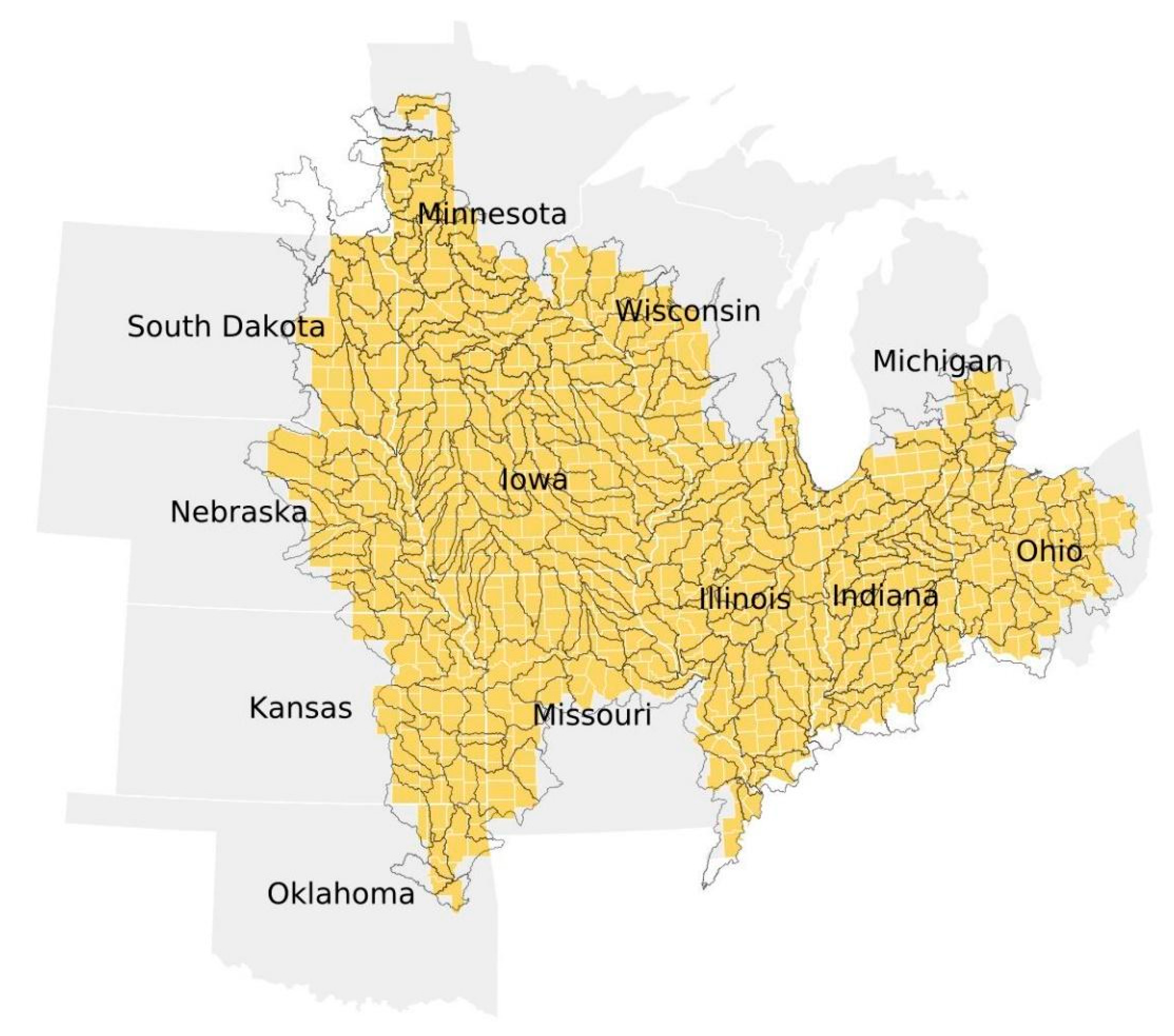
2.1. Study Area
2.2. Aggregating and Reporting
2.3. OpTIS Remote Sensing
2.3.1. Residue Cover
2.3.2. Winter Cover
2.3.3. Mapping Scale
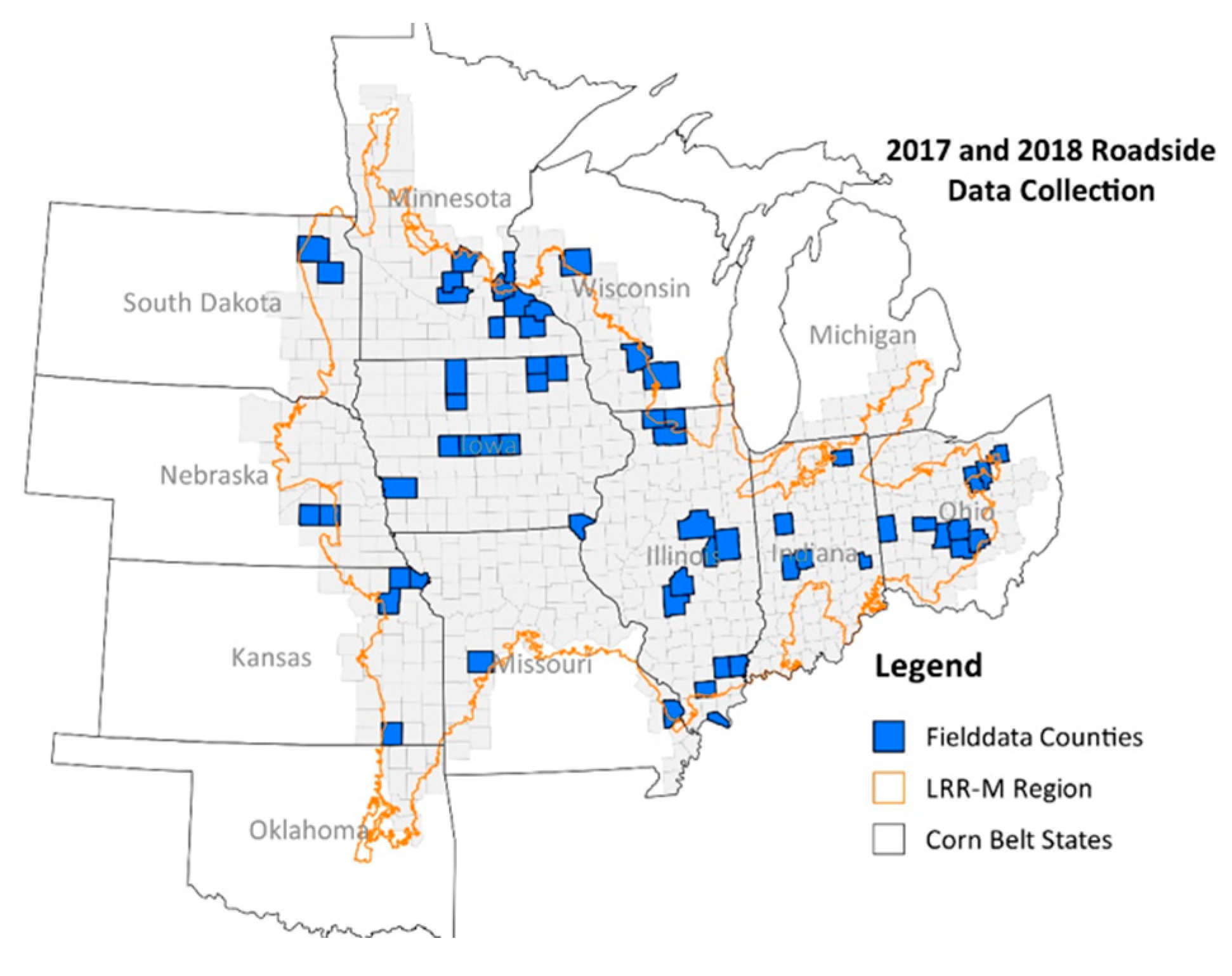
2.4. OpTIS Verification Data
2.4.1. Crop Consultants
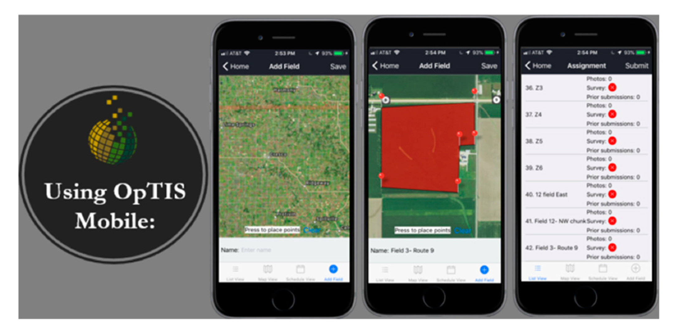
2.4.2. OpTIS Mobile Surveys
2.5. DNDC Modeling
2.5.1. Inputs and Assumptions
2.5.2. Crop Parameter Calibration
2.5.3. Management Simulations
2.5.4. Post-Processing
3. Results and Discussion
3.1. Remote Sensing Validation
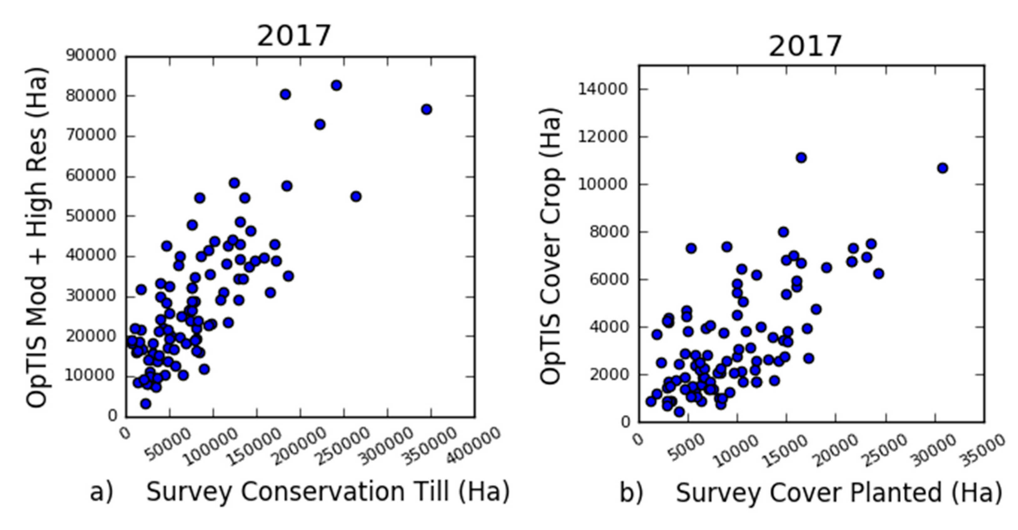
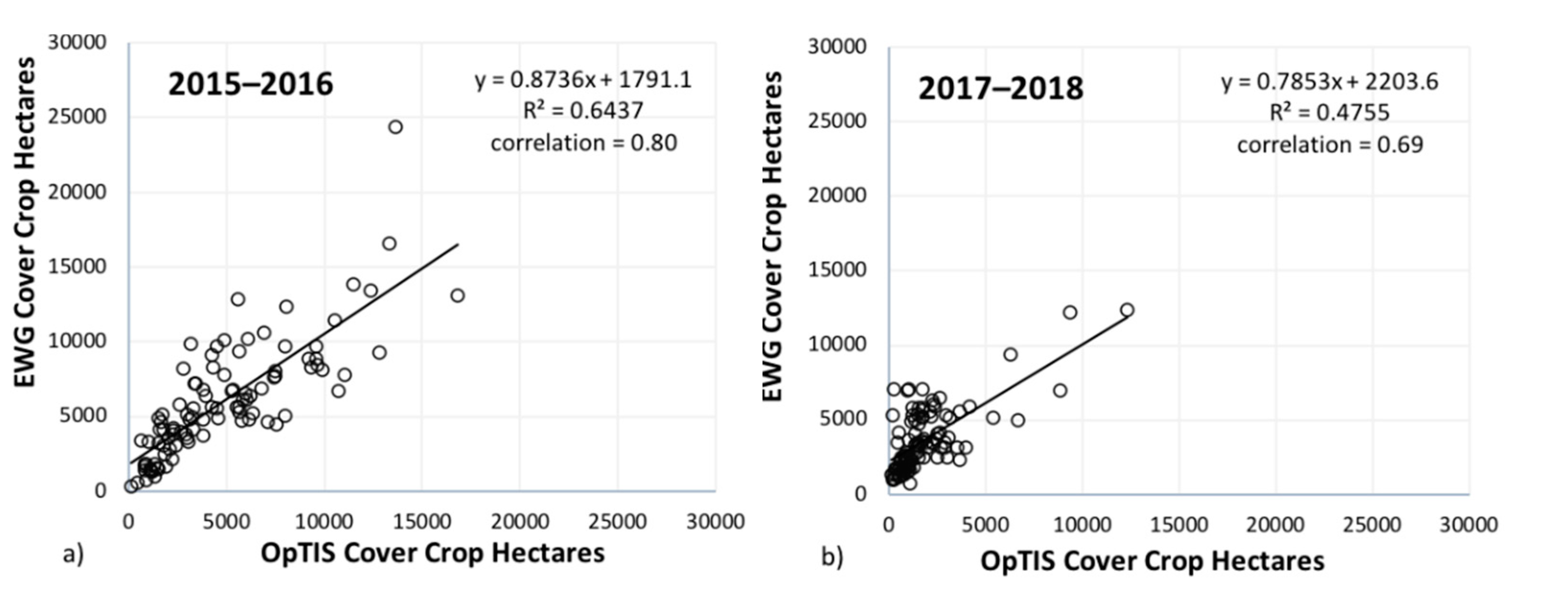
3.1.1. Cover Crops
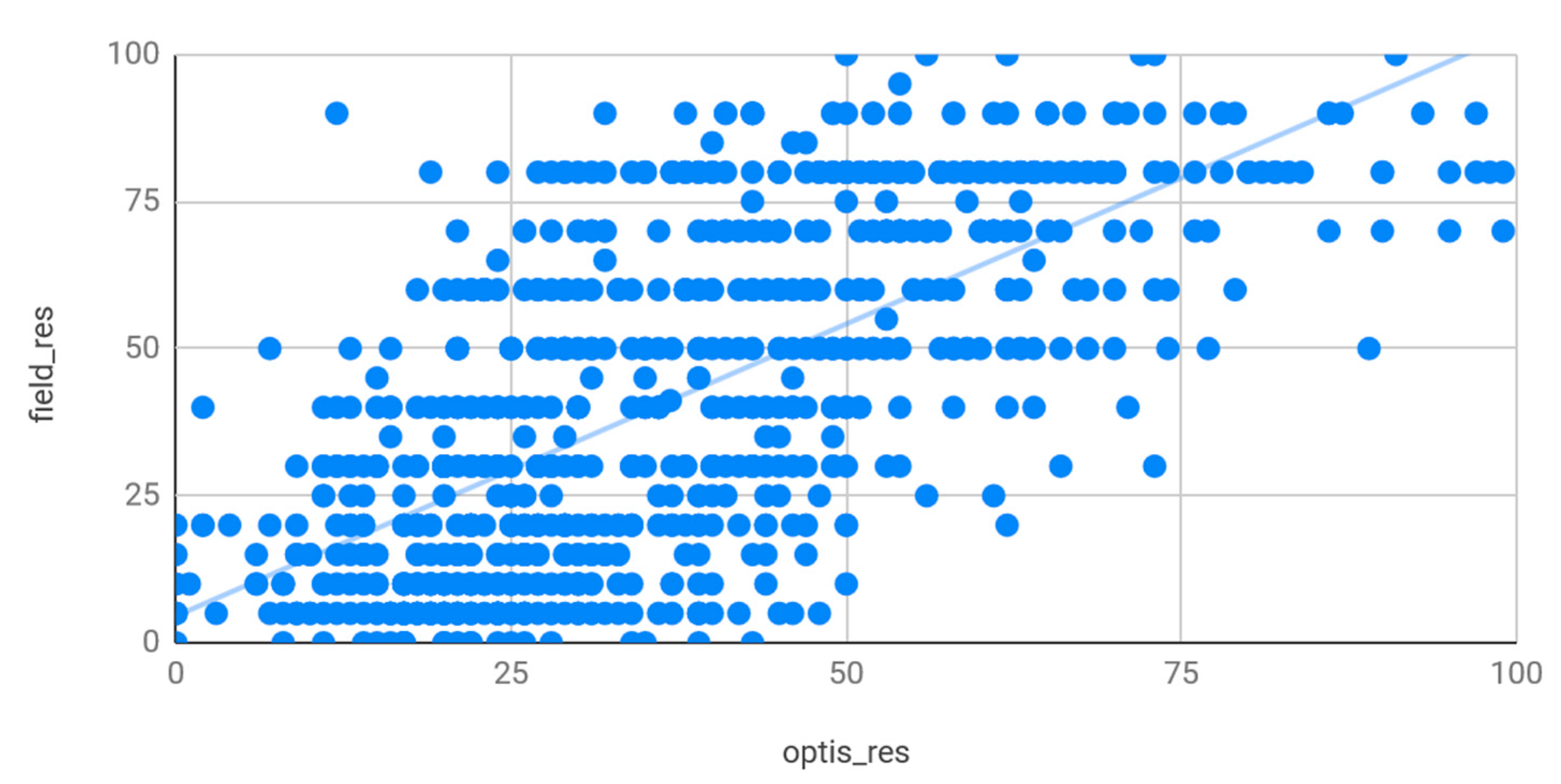
3.1.2. Residue Cover
3.1.3. Misclassification and Bias
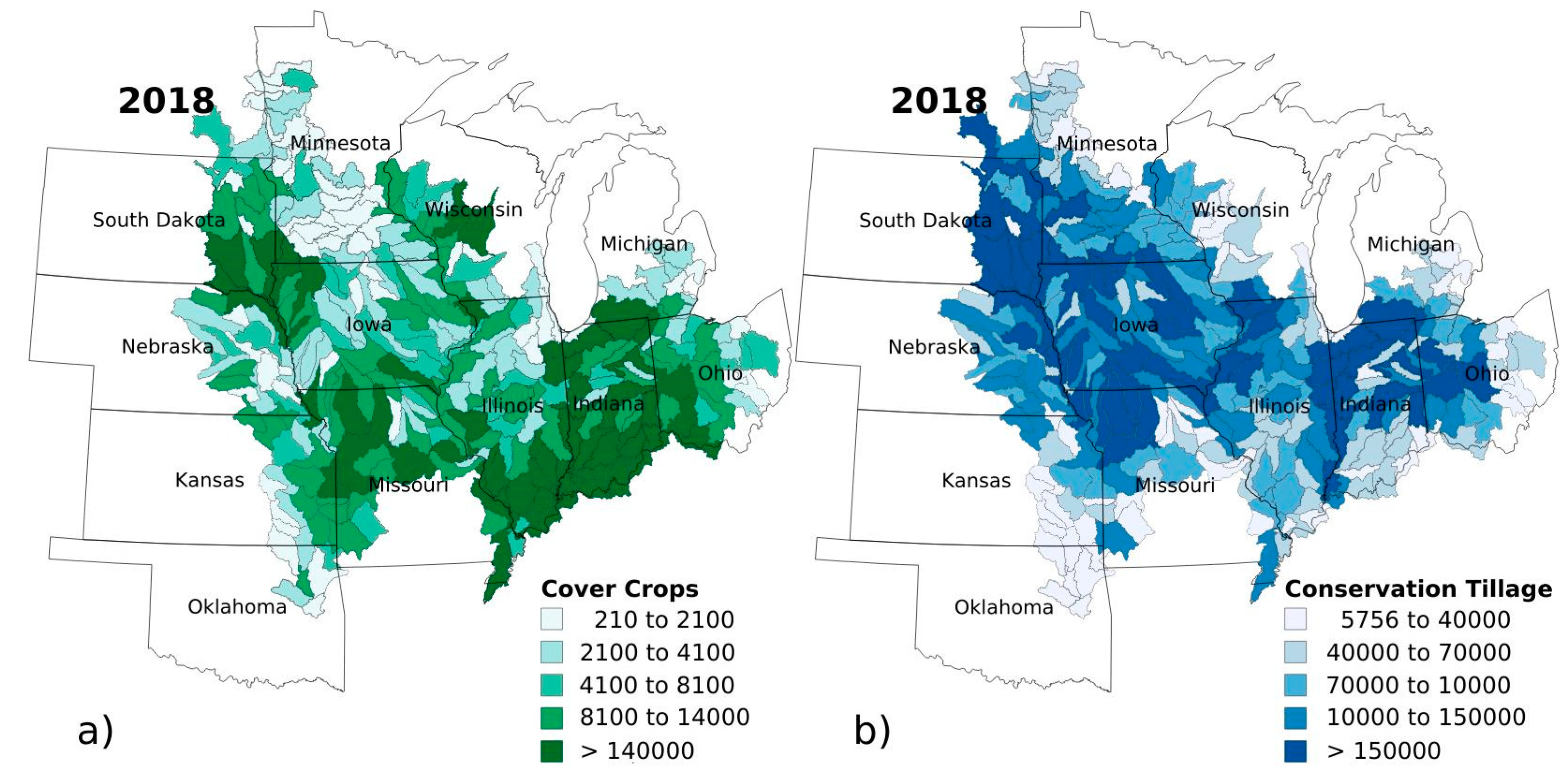
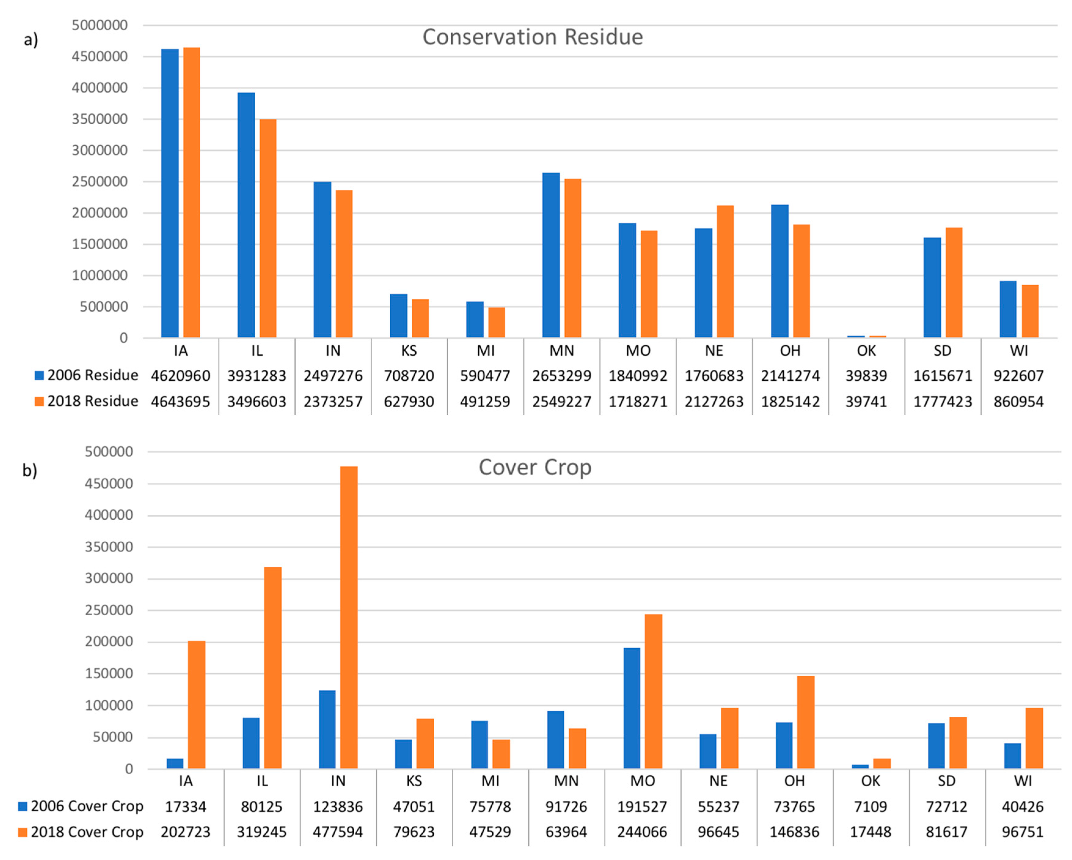
3.2. OpTIS Corn Belt Conservation Mapping Results
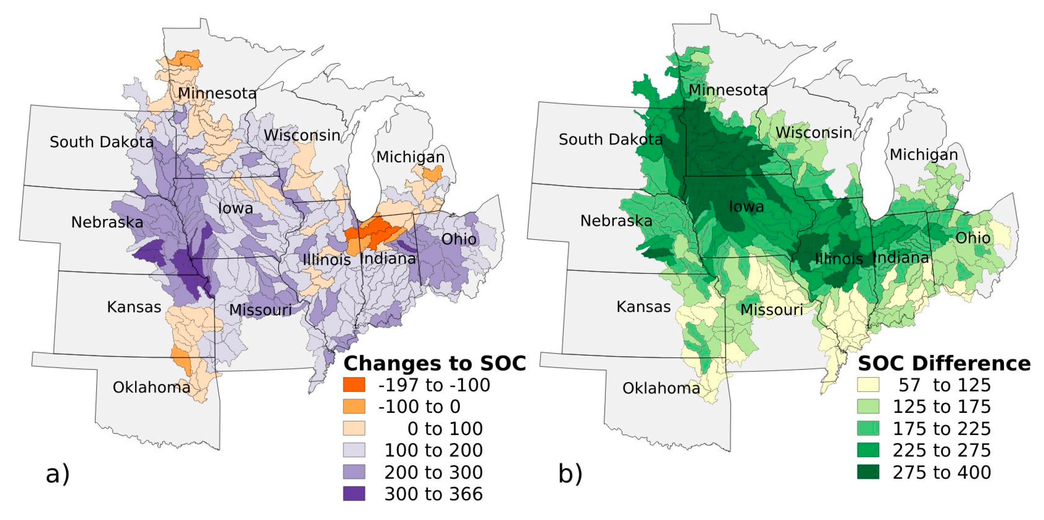
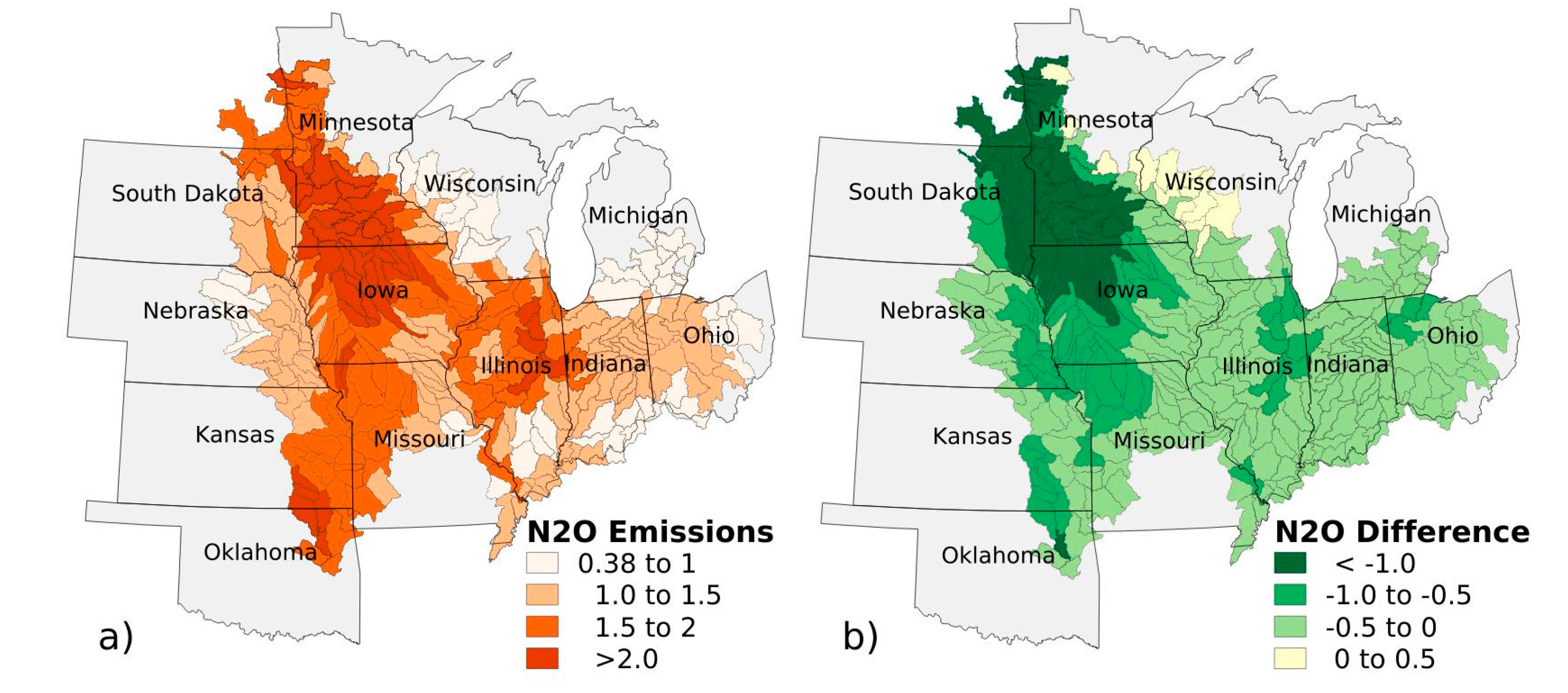
3.3. DNDC Corn Belt Conservation Mapping Results
3.4. Comparison with AgCensus and Other Mapping Efforts
3.5. Follow-on Research and Applications
4. Conclusions
Author Contributions
Funding
Acknowledgments
Conflicts of Interest
References
- Lindsey, R. Climate Change: Atmospheric Carbon Dioxide: NOAA Climate.gov. 2020. Available online: https://www.climate.gov/news-features/understanding-climate/climate-change-atmospheric-carbon-dioxide (accessed on 31 August 2020).
- Hayduk, D.; Satoyama, S.; Vafadari, K. Soils Help to Combat and Adapt to Climate Change by Playing a Key Role in the Carbon Cycle; Food and Agriculture Organization of the United Nations: Rome, Italy, 2015; pp. 1–4. Available online: http://www.fao.org/3/a-i4737e.pdf (accessed on 20 September 2019).
- Janzen, H.H. Janzen Soil carbon: A measure of ecosystem response in a changing world? Can. J. Soil Sci. 2005, 85, 467–480. [Google Scholar] [CrossRef]
- Lal, R.; Follett, R.; Stewart, B.A.; Kimble, J. Soil Carbon Sequestration to Mitigate Climate Change and Advance Food Security. Soil Sci. 2007, 172, 943–956. [Google Scholar] [CrossRef]
- Farm Service Agency (FSA). Crop Acreage Data Reported to FSA. 2019 Crop Year 2019_fsa_acres_web_010220.xlsx; United States Department of Agriculture Farm Service Agency: Washington, DC, USA, 2019. Available online: https://www.fsa.usda.gov/news-room/efoia/electronic-reading-room/frequently-requested-information/crop-acreage-data/index (accessed on 8 August 2019).
- United States Department of Agriculture (USDA). USDA Strategic Plan: FY 2018—2022; USDA: Washington DC, USA, 2018; p. 33.
- Bégué, A.; Arvor, D.; Bellon, B.; Betbeder, J.; de Abelleyra, D.; Ferraz, R.P.D.; Lebourgeois, V.; Lelong, C.; Simões, M.; Verón, S.R. Remote sensing and cropping practices: A review. Remote Sens. 2018, 10, 99. [Google Scholar] [CrossRef]
- Uri, N.D. Factors Affecting the Use of Conservation Tillage in the United States. Water Air Soil Pollut. 1999, 116, 621–638. [Google Scholar] [CrossRef]
- United States Department of Agriculture (USDA); Natural Resources Conservation Service (NRCS). Conservation Practice Standard Overview: Residue and Tillage Management (329) No-Till/Strip Till/Direct Seed. In United States Department of Agriculture Natural Resources Conservation Service; USDA: Washington, DC, USA, 2012; pp. 1–2. [Google Scholar]
- United States Department of Agriculture (USDA); Natural Resources Conservation Service (NRCS). Conservation Practice Standard Overview: Cover Crop (340); United States Department of Agriculture Natural Resources Conservation Service: Washington, DC, USA, 2014; pp. 1–2.
- Conservation Technology Information Center (CTIC). Annual Report 2019–2020 National Cover Crop Survey August 2020; Conservation Technology Information Center: West Lafayette, IN, USA, 2020; Available online: https://www.sare.org/wp-content/uploads/2019-2020-National-Cover-Crop-Survey.pdf (accessed on 4 August 2019).
- United States Department of Agriculture (USDA); Natural Resources Conservation Service (NRCS); Environmental Quality Incentives Program (EQIP). Environmental Quality Incentives Program; United States Department of Agriculture Natural Resources Conservation Service: Washington, DC, USA, 2019. Available online: https://www.nrcs.usda.gov/wps/portal/nrcs/main/national/programs/financial/eqip/ (accessed on 19 July 2019).
- Six, J.; Elliott, E.T.; Paustian, K. Agregate and Soil Organic Matter Dynamics under Conventional and No-Tillage Systems. Soil Sci. Soc. Am. J. 1999, 63, 1350–1358. [Google Scholar] [CrossRef]
- Grandy, A.S.; Robertson, G.P. Land-use intensity effects on soil organic carbon accumulation rates and mechanisms. Ecosystems 2007, 10, 58–73. [Google Scholar] [CrossRef]
- Steenwerth, K.; Belina, K. Cover crops enhance soil organic matter, carbon dynamics and microbiological function in a vineyard agroecosystem. Appl. Soil Ecol. 2008, 40, 359–369. [Google Scholar] [CrossRef]
- Hively, W.; Lang, M.; Mccarty, G.; Keppler, J.; Sadeghi, A.; McConnell, L. Using satellite remote sensing to estimate winter cover crop nutrient uptake efficiency. J. Soil Water Conserv. 2009, 64, 303–313. [Google Scholar] [CrossRef]
- Bricklemyer, R.S.; Lawrence, R.L.; Miller, P.R. Documenting no-till and conventional till practices using Landsat ETM+ imagery and logistic regression. J. Soil Water Conserv. 2002, 57, 267–271. [Google Scholar]
- Van Deventer, A.P.; Ward, A.D.; Gowda, P.M.; Lyon, J.G. Using thematic mapper data to identify contrasting soil plains and tillage practices. Photogramm. Eng. Remote Sens. 1997, 63, 87–93. [Google Scholar]
- Gowda, P.H.; Dalzell, B.J.; Mulla, D.J.; Kollman, F. Mapping tillage practices with landstat thematic mapper based logistic regression models. J. Soil Water Conserv. 2001, 56, 91–96. [Google Scholar]
- Daughtry, C.S.T.; Doraiswamy, P.; Hunt, E.; Stern, A.; McMurtrey, J.; Prueger, J. Remote sensing of crop residue cover and soil tillage intensity. Soil Tillage Res. 2006, 91, 101–108. [Google Scholar] [CrossRef]
- Hagen, S.C.; Heilman, P.; Marsett, R.; Torbick, N.; Salas, W.; Van Ravensway, J.; Qi, J. Mapping Total Vegetation Cover Across Western Rangelands with Moderate-Resolution Imaging Spectroradiometer Data. Rangel. Ecol. Manag. 2012, 65, 456–467. [Google Scholar] [CrossRef]
- Bricklemyer, R.S.; Lawrence, R.; Miller, P.R.; Battogtokh, N. Predicting tillage practices and agricultural soil disturbance in north central Montana with Landsat imagery. Agric. Ecosyst. Environ. 2006, 114, 210–216. [Google Scholar] [CrossRef]
- Bricklemyer, R.S.; Lawrence, R.L.; Miller, P.R.; Battogtokh, N. Monitoring and verifying agricultural practices related to soil carbon sequestration with satellite imagery. Agric. Ecosyst. Environ. 2007, 118, 201–210. [Google Scholar] [CrossRef]
- Azzari, G.; Grassini, P.; Edreira, J.I.R.; Conley, S.; Mourtzinis, S.; Lobell, D.B. Satellite mapping of tillage practices in the North Central US region from 2005 to 2016. Remote. Sens. Environ. 2019, 221, 417–429. [Google Scholar] [CrossRef]
- Watts, D.B.; Runion, G.B.; Balkcom, K.S. Nitrogen fertilizer sources and tillage effects on cotton growth, yield, and fiber quality in a coastal plain soil. Field Crop. Res. 2017, 201, 184–191. [Google Scholar] [CrossRef]
- Azzari, G.; Lobell, D. Landsat-based classification in the cloud: An opportunity for a paradigm shift in land cover monitoring. Remote. Sens. Environ. 2017, 202, 64–74. [Google Scholar] [CrossRef]
- Prabhakara, K.; Hively, W.D.; Mccarty, G.W. Evaluating the relationship between biomass, percent groundcover and remote sensing indices across six winter cover crop fields in Maryland, United States. Int. J. Appl. Earth Obs. Geoinf. 2015, 39, 88–102. [Google Scholar] [CrossRef]
- Allen, R.G.; Tasumi, M.; Morse, A.; Trezza, R. A Landsat-based energy balance and evapotranspiration model in Western US water rights regulation and planning. Irrig. Drain. Syst. 2005, 19, 251–268. [Google Scholar] [CrossRef]
- Li, C.; Frolking, S.; Frolking, T.A. A model of nitrous oxide evolution from soil driven by rainfall events: 1. Model structure and sensitivity. J. Geophys. Res. Space Phys. 1992, 97, 9759–9776. [Google Scholar] [CrossRef]
- Li, C.; Frolking, S.; Frolking, T.A. A model of nitrous oxide evolution from soil driven by rainfall events: 2. Model applications. J. Geophys. Res. Space Phys. 1992, 97, 9777–9783. [Google Scholar] [CrossRef]
- Li, C.; Frolking, S.; Harriss, R. Modeling carbon biogeochemistry in agricultural soils. Glob. Biogeochem. Cycles 1994, 8, 237–254. [Google Scholar] [CrossRef]
- Gilhespy, S.L.; Anthony, S.; Cardenas, L.; Chadwick, D.; Del Prado, A.; Li, C.; Misselbrook, T.; Rees, R.M.; Salas, W.; Sanz-Cobena, A.; et al. First 20 years of DNDC (DeNitrification DeComposition): Model evolution. Ecol. Model. 2014, 292, 51–62. [Google Scholar] [CrossRef]
- Giltrap, D.L.; Li, C.; Saggar, S. DNDC: A process-based model of greenhouse gas fluxes from agricultural soils. Agric. Ecosyst. Environ. 2010, 136, 292–300. [Google Scholar] [CrossRef]
- Giltrap, D.; Yeluripati, J.; Smith, P.; Fitton, N.; Smith, W.; Grant, B.; Dorich, C.D.; Deng, J.; Topp, C.F.; Abdalla, M.; et al. Global Research Alliance N 2 O chamber methodology guidelines: Summary of modeling approaches. J. Environ. Qual. 2020, 49, 1168–1185. [Google Scholar] [CrossRef]
- Yeluripati, J.B.; Del Prado, A.; Sanz-Cobena, A.; Rees, R.M.; Li, C.; Chadwick, D.; Tilston, E.; Topp, C.F.E.; Cardenas, L.M.; Ingraham, P.; et al. Global Research Alliance Modelling Platform (GRAMP): An open web platform for modelling greenhouse gas emissions from agro-ecosystems. Comput. Electron. Agric. 2015, 111, 112–120. [Google Scholar] [CrossRef][Green Version]
- Li, C. Modeling Trace Gas Emissions from Agricultural Ecosystems. Nutr. Cycl. Agroecosyst. 2000, 58, 259–276. [Google Scholar] [CrossRef]
- Li, C.; Farahbakhshazad, N.; Jaynes, D.B.; Dinnes, D.L.; Salas, W.; McLaughlin, D. Modeling nitrate leaching with a biogeochemical model modified based on observations in a row-crop field in Iowa. Ecol. Model. 2006, 196, 116–130. [Google Scholar] [CrossRef]
- Li, C.; Salas, W.; Zhang, R.; Krauter, C.; Rotz, C.A.; Mitloehner, F. Manure-DNDC: A biogeochemical process model for quantifying greenhouse gas and ammonia emissions from livestock manure systems. Nutr. Cycl. Agroecosyst. 2012, 93, 163–200. [Google Scholar] [CrossRef]
- Zhang, Y.; Li, C.; Zhou, X.; Moore, B. A simulation model linking crop growth and soil biogeochemistry for sustainable agriculture. Ecol. Model. 2002, 151, 75–108. [Google Scholar] [CrossRef]
- Li, C.; Frolking, S.; Butterbach-Bahl, K. Carbon Sequestration in Arable Soils is Likely to Increase Nitrous Oxide Emissions, Offsetting Reductions in Climate Radiative Forcing. Clim. Chang. 2005, 72, 321–338. [Google Scholar] [CrossRef]
- Zhang, F.; Li, C.; Wang, Z.; Li, X. Long-term effects of management history on carbon dynamics in agricultural soils in Northwest China. Environ. Earth Sci. 2015, 75, 1–9. [Google Scholar] [CrossRef]
- Camarotto, C.; Ferro, N.D.; Piccoli, I.; Polese, R.; Furlan, L.; Chiarini, F.; Morari, F. Conservation agriculture and cover crop practices to regulate water, carbon and nitrogen cycles in the low-lying Venetian plain. Catena 2018, 167, 236–249. [Google Scholar] [CrossRef]
- Jarecki, M.; Grant, B.; Smith, W.; Deen, B.; Drury, C.; Vanderzaag, A.C.; Qian, B.; Yang, J.; Wagner-Riddle, C. Long-term Trends in Corn Yields and Soil Carbon under Diversified Crop Rotations. J. Environ. Qual. 2018, 47, 635–643. [Google Scholar] [CrossRef]
- Deng, J.; Li, C.; Burger, M.; Horwath, W.R.; Smart, D.; Six, J.; Guo, L.; Salas, W.; Frolking, S.; Cuo, L. Assessing Short-Term Impacts of Management Practices on N 2 O Emissions from Diverse Mediterranean Agricultural Ecosystems Using a Biogeochemical Model. J. Geophys. Res. Biogeosci. 2018, 123, 1557–1571. [Google Scholar] [CrossRef]
- Deng, J.; Zhu, B.; Zhou, Z.; Zheng, X.; Li, C.; Wang, T.; Tang, J. Modeling nitrogen loadings from agricultural soils in southwest China with modified DNDC. J. Geophys. Res. Space Phys. 2011, 116. [Google Scholar] [CrossRef]
- Deng, Q.; Hui, D.; Wang, J.; Yu, C.-L.; Li, C.; Reddy, K.C.; Dennis, S. Assessing the impacts of tillage and fertilization management on nitrous oxide emissions in a cornfield using the DNDC model. J. Geophys. Res. Biogeosci. 2016, 121, 337–349. [Google Scholar] [CrossRef]
- Abalos, D.; Smith, W.N.; Grant, B.B.; Drury, C.F.; Mackell, S.; Wagner-Riddle, C. Scenario analysis of fertilizer management practices for N2O mitigation from corn systems in Canada. Sci. Total Environ. 2016, 573, 356–365. [Google Scholar] [CrossRef]
- He, W.; Yang, J.Y.; Drury, C.F.; Smith, W.; Grant, B.; He, P.; Qian, B.; Zhou, W.; Hoogenboom, G. Estimating the impacts of climate change on crop yields and N2O emissions for conventional and no-tillage in Southwestern Ontario, Canada. Agric. Syst. 2018, 159, 187–198. [Google Scholar] [CrossRef]
- Beheydt, D.; Boeckx, P.; Sleutel, S.; Li, C.; Vancleemput, O. Validation of DNDC for 22 long-term N2O field emission measurements. Atmos. Environ. 2007, 41, 6196–6211. [Google Scholar] [CrossRef]
- Wang, J.; Cardenas, L.M.; Misselbrook, T.; Cuttle, S.; Thorman, R.E.; Li, C. Modelling nitrous oxide emissions from grazed grassland systems. Environ. Pollut. 2012, 162, 223–233. [Google Scholar] [CrossRef] [PubMed]
- Cai, Z.; Sawamoto, T.; Li, C.; Kang, G.; Boonjawat, J.; Mosier, A.R.; Wassmann, R.; Tsuruta, H. Field validation of the DNDC model for greenhouse gas emissions in East Asian cropping systems. Glob. Biogeochem. Cycles 2003, 17, 1–10. [Google Scholar] [CrossRef]
- Ingraham, P.A.; Salas, W.A. Assessing nitrous oxide and nitrate leaching mitigation potential in US corn crop systems using the DNDC model. Agric. Syst. 2019, 175, 79–87. [Google Scholar] [CrossRef]
- United States Department of Agriculture (USDA); Service Center Agencies National Geospatial Management Center. 8 Digit Watershed Boundary Dataset; USDA/NRCS—National Geospatial Management Center: Reston, VA, USA, 2013.
- Drusch, M.; Del Bello, U.; Carlier, S.; Colin, O.; Fernandez, V.; Gascon, F.; Hoersch, B.; Isola, C.; Laberinti, P.; Martimort, P.; et al. SENTINEL-2: ESA’s Optical High-Resolution Mission for GMES Operational Services. Remote Sens. Environ. 2012, 120, 25–36. [Google Scholar] [CrossRef]
- PRISM Climate Group, Oregon State University. Available online: http://prism.oregonstate.edu (accessed on 4 August 2019).
- United States Department of Agriculture (USDA); National Agricultural Statistics Service (NASS); Cropland Data Layer (CDL). Published Crop-Specific Data Layer; USDA-NASS: Washington, DC, USA, 2019. Available online: https://nassgeodata.gmu.edu/CropScape/ (accessed on 5 August 2019).
- NADP Program Office Wisconsin State Laboratory of Hygiene. National Atmospheric Deposition Program (NRSP-3); NADP Program Office Wisconsin State Laboratory of Hygiene: Madison, WI, USA, 2020. [Google Scholar]
- United States Department of Agriculture (USDA); National Agricultural Statistics Service (NASS). NASS—Quick Stats. 2018. Available online: https://data.nal.usda.gov/dataset/nass-quick-stats. (accessed on 13 November 2018).
- United States Department of Agriculture (USDA); National Agricultural Statistics Service. Crop Production Historical Track Record; US Gov. Print. Office: Washington, DC, USA, 2016.
- United States Department of Agriculture (USDA); Economic Research Service (ERS). Fertilizer Use and Price Website. 2017. Available online: https://www.ers.usda.gov/data-products/fertilizer-use-and-price.aspx (accessed on 2 January 2017).
- United States Department of Agriculture (USDA); National Agricultural Statistics Service (NASS). Field Crops: Usual Planting and Harvesting Dates, October 2010; Agricultural Handbook Number 628; United States Department of Agriculture National Agricultural Statistics Service: Washington, DC, USA, 2010.
- Soil Survey Staff, Natural Resources Conservation Service, United States Department of Agriculture. Soil Survey Geographic (SSURGO) Database; United States Department of Agriculture: Washington, DC, USA, 2018. Available online: https://sdmdataaccess.sc.egov.usda.gov (accessed on 15 December 2018).
- Keeling, C.D.; Piper, S.C.; Bacastow, R.B.; Wahlen, M.; Whorf, T.P.; Heimann, M.; Meijer, H.A. Exchanges of Atmospheric CO2 and 13 CO2 with the Terrestrial Biosphere and Oceans from 1978 to 2000. I. Global Aspects; SIO Reference Series, No. 01-06; Scripps Institution of Oceanography: San Diego, CA, USA, 2001; 88p, Available online: http://escholarship.org/uc/item/09v319r9 (accessed on 5 July 2019).
- Abendroth, L.J.; Herzmann, D.E.; Chighladze, G.; Kladivko, E.J.; Helmers, M.J.; Bowling, L.; Castellano, M.; Cruse, R.M.; Dick, W.A.; Fausey, N.R.; et al. Sustainable Corn CAP Research Data (USDA-NIFA Award No. 2011-68002-30190); National Agricultural Library-ARS-USDA: Beltsville, MD, USA, 2017. [Google Scholar] [CrossRef]
- Pribyl, D.W. A Critical review of the conventional SOC to SOM conversion factor. Geoderma 2010, 156, 75–83. [Google Scholar] [CrossRef]
- Iowa State University. Corn Nitrogen Rate Calculator. 2019. Available online: http://cnrc.agron.iastate.edu/ (accessed on 18 February 2019).
- Pervez, M.S.; Brown, J.F. Mapping Irrigated Lands at 250-m Scale by Merging MODIS Data and National Agricultural Statistics. Remote Sens. 2010, 2, 2388–2412. [Google Scholar] [CrossRef]
- Saxton, K.E.; Rawls, W.J. Soil water characteristic estimates by texture and organic matter for hydrologic solutions. Soil Sci. Soc. Am. J. 2006, 70, 1569–1578. [Google Scholar] [CrossRef]
- Stehman, S. Selecting and interpreting measures of thematic classification accuracy. Remote Sens. Environ. 1997, 62, 77–89. [Google Scholar] [CrossRef]
- Pontius, R.G.; Millones, M. Death to Kappa: Birth of quantity disagreement and allocation disagreement for accuracy assessment. Int. J. Remote Sens. 2011, 32, 4407–4429. [Google Scholar] [CrossRef]
- Deines, J.M.; Wang, S.; Lobell, D.B. Satellites reveal a small positive yield effect from conservation tillage across the US Corn Belt. Environ. Res. Lett. 2019, 14. [Google Scholar] [CrossRef]
- Chae, K.; Cisney, J.; Gang, A.; Khan, K.; Lloyd, T.; Mckay, N.; Mckeen, G.; Ossanna, J.; Owen, J.; Pan, S.; et al. State Sustainability Index. 2016. Available online: https://drive.google.com/file/d/0B_41G9iz2F6PbWxjNXVaZnRqdzQ/view (accessed on 9 October 2020).


| Data Product | Technology | Source | Website/Access |
|---|---|---|---|
| Landsat | OpTIS | USGS/NASA | https://earthexplorer.usgs.gov/ |
| MODIS | OpTIS | NASA | modis.gsfc.nasa.gov/data/ |
| Sentinel 2 | OpTIS | ESA [54] | sentinel.esa.int/web/sentinel/sentinel-data-access |
| PRISM | OpTIS & DNDC | Oregon State University [55] | http://www.prism.oregonstate.edu/ |
| Cropland Data Layer (CDL) | OpTIS & DNDC | USDA [56] | www.nass.usda.gov/Research_and_Science/Cropland/SARS1a.php |
| MIrAD-US | DNDC | USGS | https://earlywarning.usgs.gov/fews/search |
| N deposition | DNDC | NADP [57] | http://nadp.slh.wisc.edu/ntn/ |
| Annual survey, crop yield, fertilizer, harvested acres, irrigated status | DNDC | USDA NASS [58,59] | quickstats.nass.usda.gov/ |
| Fertilizer type | DNDC | USDA ERS [60] | https://www.ers.usda.gov/data-products/fertilizer-use-and-price/ |
| Plant and harvest dates | DNDC | USDA NASS [61] | Field Crops, Usual Planting and Harvesting Dates, October 2010—Agricultural Handbook Number 628 |
| SSURGO | DNDC | USDA NRCS [62] | www.nrcs.usda.gov/wps/portal/nrcs/detail/soils/survey/geo/?cid=nrcs142p2_053628 |
| Atmospheric CO2 | DNDC | Scripps Inst. Of Oceanography [63] | http://scrippsco2.ucsd.edu/data/atmospheric_co2/primary_mlo_co2_record |
| Crop biomass data | DNDC | Sustainable Corn Coordinated Agricultural Project (CAP) Team Research Data [64] | https://datateam.agron.iastate.edu/cscap/ |
| DNDC Management Scenarios | |
|---|---|
| OpTIS-mapped | “Actual” distribution of soil health management practices in the study area |
| All ConvTill | First alternative scenario assumed conventional tillage all the time |
| No CC | Second alternative scenario assumed no cover cropping |
| All ConvTill & No CC | Third alternative scenario combined the first two alternative scenarios Simulated conventional tillage and no cover cropping across all years |
| Cover Crop Classification (n = 959) | Field Data (Actual Values) | ||
|---|---|---|---|
| Positive (1) | Negative (0) | ||
| OpTIS (Predicted values) | Positive (1) | TP = 139 | FP = 22 |
| Negative (0) | FN = 92 | TN = 706 | |
| Classification Metric | Formula | Value |
|---|---|---|
| Sensitivity | TP/TP + FN | 0.60 |
| Specificity | TN/TN + FP | 0.97 |
| Accuracy | TP + TN/total | 0.88 |
| Precision | TP/TP + FP | 0.86 |
| F-measure | 2 ∗ Sensitivity ∗ Precision/Recall + Precision | 0.71 |
| False-Positive Rate | 1-Specificity | 0.03 |
| Years | Cover Crop Acres | Cover Crop Ha | % Area of Cover Crops | Conservation Tillage Acres | Conservation Tillage Hectares | % Area of Conservation Tillage |
|---|---|---|---|---|---|---|
| 2005 | 2,065,432 | 835,869 | 2% | 48,707,764 | 19,711,762 | 42% |
| 2006 | 1,963,643 | 794,675 | 2% | 55,116,662 | 22,305,408 | 46% |
| 2007 | 784,100 | 317,321 | 1% | 48,887,840 | 19,784,638 | 42% |
| 2008 | 1,693,953 | 685,533 | 1% | 59,514,473 | 24,085,177 | 51% |
| 2009 | 853,474 | 345,396 | 1% | 59,201,973 | 23,958,710 | 51% |
| 2010 | 799,084 | 323,385 | 1% | 60,671,511 | 24,553,424 | 51% |
| 2011 | 1,156,283 | 467,941 | 1% | 56,769,756 | 22,974,406 | 47% |
| 2012 | 1,908,452 | 772,340 | 2% | 58,823,578 | 23,805,576 | 49% |
| 2013 | 2,383,074 | 964,417 | 2% | 65,479,475 | 26,499,180 | 54% |
| 2014 | 1,620,402 | 655,768 | 1% | 63,432,404 | 25,670,742 | 52% |
| 2015 | 1,050,637 | 425,187 | 1% | 66,168,899 | 26,778,187 | 55% |
| 2016 | 3,456,192 | 1,398,702 | 3% | 53,860,483 | 21,797,039 | 45% |
| 2017 | 4,872,734 | 1,971,968 | 4% | 54,391,780 | 22,012,052 | 45% |
| 2018 | 3,888,410 | 1,573,618 | 3% | 54,202,762 | 21,935,557 | 44% |
Publisher’s Note: MDPI stays neutral with regard to jurisdictional claims in published maps and institutional affiliations. |
© 2020 by the authors. Licensee MDPI, Basel, Switzerland. This article is an open access article distributed under the terms and conditions of the Creative Commons Attribution (CC BY) license (http://creativecommons.org/licenses/by/4.0/).
Share and Cite
Hagen, S.C.; Delgado, G.; Ingraham, P.; Cooke, I.; Emery, R.; P. Fisk, J.; Melendy, L.; Olson, T.; Patti, S.; Rubin, N.; et al. Mapping Conservation Management Practices and Outcomes in the Corn Belt Using the Operational Tillage Information System (OpTIS) and the Denitrification–Decomposition (DNDC) Model. Land 2020, 9, 408. https://doi.org/10.3390/land9110408
Hagen SC, Delgado G, Ingraham P, Cooke I, Emery R, P. Fisk J, Melendy L, Olson T, Patti S, Rubin N, et al. Mapping Conservation Management Practices and Outcomes in the Corn Belt Using the Operational Tillage Information System (OpTIS) and the Denitrification–Decomposition (DNDC) Model. Land. 2020; 9(11):408. https://doi.org/10.3390/land9110408
Chicago/Turabian StyleHagen, Stephen C., Grace Delgado, Peter Ingraham, Ian Cooke, Richard Emery, Justin P. Fisk, Lindsay Melendy, Thomas Olson, Shawn Patti, Nathanael Rubin, and et al. 2020. "Mapping Conservation Management Practices and Outcomes in the Corn Belt Using the Operational Tillage Information System (OpTIS) and the Denitrification–Decomposition (DNDC) Model" Land 9, no. 11: 408. https://doi.org/10.3390/land9110408
APA StyleHagen, S. C., Delgado, G., Ingraham, P., Cooke, I., Emery, R., P. Fisk, J., Melendy, L., Olson, T., Patti, S., Rubin, N., Ziniti, B., Chen, H., Salas, W., Elias, P., & Gustafson, D. (2020). Mapping Conservation Management Practices and Outcomes in the Corn Belt Using the Operational Tillage Information System (OpTIS) and the Denitrification–Decomposition (DNDC) Model. Land, 9(11), 408. https://doi.org/10.3390/land9110408