Abstract
Land change models commonly model the expected quantity of change as a Markov chain. Markov transition probabilities can be estimated by tabulating the relative frequency of change for all transitions between two dates. To estimate the appropriate transition probability matrix for any future date requires the determination of an annualized matrix through eigendecomposition followed by matrix powering. However, the technique yields multiple solutions, commonly with imaginary parts and negative transitions, and possibly with no non-negative real stochastic matrix solution. In addition, the computational burden of the procedure makes it infeasible for practical use with large problems. This paper describes a Regression-Based Markov (RBM) approximation technique based on quadratic regression of individual transitions that is shown to always yield stochastic matrices, with very low error characteristics. Using land cover data for the 48 conterminous US states, median errors in probability for the five states with the highest rates of transition were found to be less than 0.00001 and the maximum error of 0.006 was of the same order of magnitude experienced by the commonly used compromise of forcing small negative transitions estimated by eigendecomposition to 0. Additionally, the technique can solve land change modeling problems of any size with extremely high computational efficiency.
1. Introduction
Land change models are developed both as a means of understanding the drivers of land cover change, and as a means of predicting potential future scenarios of land cover [1]. Projecting where land cover will change may be modeled either empirically or theoretically. However, a key component of a land change model is the ability to estimate the amount of expected change over a specified time interval for every land transition of interest. A common approach is Markov chain analysis [1,2] where historical land cover change is used to develop a transition probability matrix that expresses the relative frequency of transitions between land cover categories over time. When the future projection is an integer multiple of the historical time frame examined, the mathematical development of the transition probability matrix is straightforward. However, there are times when the future projection needs to be for a time that does not coincide with an integer multiple of the historical time frame. For example, a specific future scenario might be of interest, such as 2050, that does not coincide with an integer multiple. Similarly, if a regional projection is being developed based on a set of subregions where the historical data are from differing periods, the projection forward to a common future scenario may involve non-integer time periods. Unfortunately, when the future time period of interest is not an integer multiple of the historical time frame, the process is much more difficult.
Figure 1 illustrates the basic requirements for a Markov chain analysis. Given two land cover maps (for 2001 and 2011 for the state of Florida in the United States in this example), a crosstabulation of the k land covers at pixels in 2001 and their corresponding land covers in 2011 allows the construction of a k × k matrix of relative frequencies of transitions between the two dates. Thus, for example, 14.91% of forest in 2001 transitioned to shrub/grass in 2011. If the projection forward in time were 10 years, to 2021, then this table could be used as the transition probability matrix. Thus, it would be expected that an additional 14.91% of remaining forest would transition to shrub/grass. However, if the projection forward were to 2031 (20 years), the expected transition probability matrix would be the square of the base matrix. In this case, 25.21% of forest in 2011 would be expected to transition to shrub/grass by 2031. In general, if P is the base transition probability matrix, then:
is the expected transition probability matrix (P′) for n steps beyond the historical period [3].

Figure 1.
A transition probability matrix for land cover change in Florida, USA, from 2001 to 2011 based on the land cover maps depicted. Florida is one of the lower 48 conterminous states, highlighted in red in the inset. The state centroid (marked with a yellow dot) is at 28.68° N, 82.46° W.
When the projection forward is not an integer multiple of the base time frame, a potential solution is to estimate the annual rate of change and then to use the power rule to project forwards for the correct number of years [4,5]. Based on the relationship expressed in Equation (1), given a base transition matrix over t years, Pt, the annual transition matrix P1 can be determined as:
The difficult part of this relationship is the need to take a tth root of the base matrix. Currently, there are two mathematical approaches to solve this problem [6]. One is to use matrix logarithms and exponentials:
where logm is the matrix logarithm and expm is the matrix exponential. The other is to use eigendecomposition [5,6]:
where λi is the ith eigenvalue of matrix Pt (the base matrix for t years) and U is a k × k eigenmatrix, given k land cover classes. However, as discussed by Takada et al. [6], these two comparable approaches can present problems. Using eigendecomposition, encoded into a computer program called TAM, they showed that mathematically there are multiple solutions for estimation of the annual rate of change on the order of tk, where t is the number of years between the two historical land covers examined (10 years in the above example), and k is the number of land cover classes (7 in this example). Thus, for the example with Florida, there are ten million (107) annual solutions, all of which obey the power rule to yield the base matrix. Many of these are complex number solutions and of those that are real, some involve negative transition probabilities. This is not reasonable since Markov transition probability matrices are stochastic matrices, which are defined by being composed entirely of non-negative real numbers that sum to 1 across each row [7]. Takada et al. [6] also indicate that it is possible that more than one stochastic annual transition matrix may be found, or indeed that none will be found. In a follow-up study, Hasegawa et al. [8] found that only 11% of 62 cases examined produced stochastic matrices. However, they showed that by forcing small negative transitions to be 0, it was possible to increase this number to 87%. That said, the biggest issue is the computational burden of the procedure used. Hasegawa et al. [8] cite an example of solving a case with 10 classes over 24 years requiring over 1000 days for computation.
To summarize, the standard approach to producing a projected Markov transition probability matrix for any arbitrary date into the future is through mathematical determination of the annualized rate (such as through eigendecomposition), and then to power the matrix to the desired date using Equation (1). However, there are several problems with the approach:
- Mathematical solution yields multiple results, many of which involve complex numbers and negative transition probabilities. Such matrices are unusable for land cover modeling of future transitions.
- It is possible that no non-negative real stochastic solution can be achieved. In these cases, an approximation can sometimes be achieved by forcing small negative transition probabilities to 0.
- Most importantly, for computational reasons, solutions are only feasible when either or both the historical time period and the number of land cover classes are very small.
This paper describes an alternative Regression-Based Markov (RBM) approximate solution that was developed as part of the IDRISI (MARKOV module) and Land Change Modeler applications inside the TerrSet software suite [9]. The procedure has none of these limitations. It is quick and always produces a stochastic matrix, based on polynomial regression. It can also solve any size problem, which is a severe limitation for mathematical solutions. However, it is an approximation, and while the general logic of the system has been very briefly discussed in the TerrSet help system [9] and elsewhere [10,11,12,13], it has never been fully described and has never been formally evaluated. This paper seeks to address this gap with a description and evaluation of the procedure in TerrSet version 19.0.2. To our knowledge, the approach is unique and with this analysis we seek to establish how closely the result approaches the correct solution when a mathematical solution is possible. As of the time of this writing, over 1600 articles are listed in Google Scholar that reference the Land Change Modeler (such as [14,15,16,17,18]), for which the RBM algorithm is a critical component. Thus, it is very important to establish its limitations. As we will show, the approach provides a high-quality approximation that always provides a solution, and which overcomes the prohibitive computational hurdle faced by mathematical approaches.
2. Regression-Based Markov
The Regression-Based Markov (RBM) approach substitutes statistical characterization and prediction for a mathematical solution for transition probability estimation. The basic logic of the algorithm is to use the power rule (Equation (1)) to generate three exact transition matrices that surround the future time period of interest. These are referred to as the control matrices. A series of quadratic regressions [19] (second-order polynomial) is then fit to the three values over time at each cell in the matrices as follows:
where pijt represents the transition probability for land cover i transitioning to land cover j at time step t, where t assumes values of 0, 1 and 2 for the three matrices generated. Since there are three data points for each transition, the regression will yield a perfect fit. The fitted equation is then used to estimate the transition probability for any period of time between these control matrices. Since the transition has k × k entries, a total of k2 regressions are computed. Figure 2 illustrates this concept.
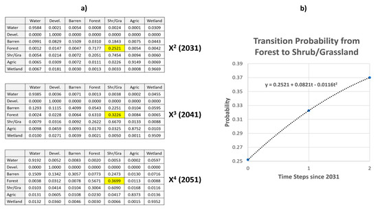
Figure 2.
An illustration of the logic of the Regression-Based Markov (RBM) algorithm. (a) To estimate the transition probability from forest to shrub/grassland in 2035, the base matrix (Figure 1) is taken to the powers of 2, 3 and 4. In each matrix, the rows represent land cover in 2001 and the columns represent land cover at the later date specified. (b) The values in the three powered matrices (an example is highlighted in yellow) are then regressed against time expressed in 10-year steps from 2031. The value for 2035 would use the fitted equation using a value of 0.4 for the value of t (since 2035 is 4/10 of the time from 2031 to 2051). The predicted transition probability is 0.2831.
As an example, consider the case of trying to generate a transition probability matrix for the year 2035 for the example with Florida (Figure 2). The year 2035 is 24 years beyond the end of the historical period, 2011. The base probability matrix in Figure 1 would be raised to the 2nd, 3rd and 4th powers to get the proper control matrices for 2031, 2041 and 2051. Predicted transition potentials would then be generated for the 49 transitions associated with this 7 × 7 table using a value of 0.4 as the value for t in Equation (2) since 2035 is 4/10 of the way between 2031 and 2041.
In a case where the target projection is less than one complete time step (10 years in the Florida case), an identity matrix is used for the first matrix, while the base matrix would be used for the second matrix and the base matrix squared would be used for the third. With this logic, the regression is only ever used for interpolation, and never extrapolation. The identity matrix has values of one along the diagonal and zero elsewhere. The rational for using the identity matrix is that if the passage of time is 0, the probability of each land cover remaining the same is 1.0 and the probability of transitioning to another category is 0.0. It is also known that any square matrix to the power of 0 is an identity matrix [20]. Figure 3 provides a schematic to illustrate the algorithm for all three variants based on the relationship between the projection date and the historical time frame.

Figure 3.
Schematic of the RBM algorithm for cases where the future date is between: (a) the present and one time step ahead, (b) one and two time steps ahead, and (c) x and x + 1 time steps ahead. The input land cover maps are shown in light blue. Analytical operations are symbolized in green. Dark blue symbols represent transition probability matrices. With this logic, the future transition probability matrix is always interpolated, using quadratic regression, between control matrices P0 and P1. Note that recursive matrix powering is required in (b) and (c) to generate control matrices.
3. Materials and Methods
3.1. Study Area and Data
To test the quality of the RBM procedure, National Land Cover Database (NLCD) land cover maps [21] for each of the 48 conterminous states in the United States were acquired for 2001 and 2011 at a 30-m resolution. Because of computational limitations of the TAM procedure (as will be discussed below), the NLCD original land cover classes were reclassified to 7 broad classes. Base transition probability maps were then created for this 10-year period for each of the 48 states using crosstabulation. Each of these base probability maps was submitted to the TAM computer software developed by [6] to determine which states had a stochastic solution for the annual matrix. For all cases where a single stochastic matrix solution was achieved, the result was accepted as the true annualized transition matrix, and all powers of that matrix necessary for testing were assumed to be true within the limits of computational precision.
In total, 42 states were found to have a single stochastic solution for the annualized matrix. The ones that did not were Arkansas, Louisiana, Maine, Montana, Rhode Island and Washington. Of the 42 states with single stochastic annual transition probability matrices, the five with the highest rates of transition were (highest to lowest) Alabama, Georgia, Florida, Delaware and Arizona. This was assessed by looking at the mean transition probabilities for each state along the diagonal. Since these entries express persistence, the states with the lowest mean diagonal values were thus the states with the highest rates of transition. Note however, that this analysis was not area weighted. The intention was to find the states with the most extreme transitions to model rather than the greatest quantity of change. These five states were then selected for detailed examination. Figure 1 illustrates the data for the state of Florida—a state typical of this group.
3.2. Data Analysis
The first goal of the analysis was to determine the degree to which the quadratic model fits the evolution of transition potentials over time between the three control matrices. Control matrices for 2011 (an identity matrix), 2021 (the base 10-year transition matrix) and 2031 (the base matrix squared) were considered. Then, the annualized transition matrices from the TAM program [6] were used to create transition matrices at 1-year intervals for the intervening years from 2011 to 2031 for the 5 focus states. Thus, for each of the 49 cells in the 7 × 7 matrix of transitions, 21 data points were available over time. Quadratic regressions were then fitted over these 21 points for each of the 49 transitions and each of the 5 states, yielding a total of 245 regressions. The Adjusted R2 was then calculated to determine the goodness of fit. Since the TAM results are understood to be the true values, this allows a determination of the degree to which a quadratic regression fits the true evolution of the transition probabilities over the span of three control matrices.
The second goal of the analysis was to determine the nature of the error associated with the RBM algorithm. For comparison with the 21 transition matrices from 2011 to 2031 generated by TAM over the 5 states, the RBM procedure was used to generate corresponding transition matrices. These could then be differenced to evaluate the nature of the error introduced by the RBM procedure. The rationale for estimating over a 20-year period was that with a 10-year base period, the first half (2012–2020) would require the use of an identity matrix for the first of the three transition matrices used in the regression, while the second half (2021–2030) would use the base transition matrix as the first of the three control matrices.
4. Results
Using the TAM annualized transition matrices for each of the five focus states, matrix powering with exponents from 0 to 20 was used to create annual transition probability matrices from 2011 to 2031. The exponent of 0 yields an identity matrix. Quadratic regressions were then fit using the 21 data points over time for each of the 7 × 7 = 49 transitions and for each of the 5 focus states. Thus, a total of 245 regressions were assessed. The resulting Adjusted R2 values were all above 99%, with the lowest value being from shrub/grassland to barren in Georgia with an Adjusted R2 of 99.94%. Figure 4 illustrates this regression. As can be seen, the fit is exceptionally good.
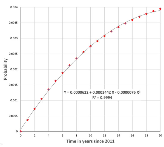
Figure 4.
Evolution of the probability of transition from shrub/grassland to barren in Georgia as determined from the TAM program for durations from 1 to 20 years and set to 0 for 0 years (markers) along with the quadratic fit determined by the RBM procedure.
To assess the error associated with the RBM estimate, the RBM algorithm was used to generate similar estimates of transition probability matrices for the 21 years from 2011 to 2031 for each of the five focus states. The absolute differences from the known true values using the TAM procedure [6] were then determined for each year over the 49 transitions. Maximum, mean and median values were then determined for each year in each state. Figure 5 shows the error distribution for Georgia, being the state with the worst fit encountered. The other four focus states all have a similar distribution shape, but with lower errors. Their corresponding graphs can be found in Figures S1–S4 in the Supplementary Materials. In addition, Table 1 tabulates the highest of these values across the five focus states.

Figure 5.
Maximum, mean and median error in transition probability estimation for all 49 transitions in Georgia, USA from 2011 to 2021.

Table 1.
Highest median, mean and maximum errors in transition probability across all 49 transitions, by state.
5. Discussion
It is clear from the results that a quadratic regression fits the evolution of transition probabilities over differing durations of time very well. The worst model fit had an Adjusted R2 of 99.94%. Comparing the fitted transition probabilities to the correct values as computed by TAM (Table 1), half the errors in each of the five focus states (as measured by the median) were less than 0.00001 and no errors were as high as one percent (the maximum was 0.006).
This raises the question of what constitutes an acceptable error. The authors in [7] describe an approximation commonly used in the medical field in which the individual probabilities p in the base matrix P are used to estimate their annual equivalent probabilities p1 using the following formula:
where t is the number of years between the historical periods used to compute the base transition matrix. Using this procedure for the transition with the maximum RBM error encountered in Georgia, the error resulting from Equation (6) was 0.028—well above 1% and almost five times higher than that encountered using RBM.
The TAM procedure [6] is also an approximation whenever small negative transition probabilities are found. Negative values between -0.1 and 0 are forced to 0 and then the affected row category is renormalized so that the row probabilities sum to 1. In theory, an adjustment to a transition probability in the TAM procedure could be as high as 0.1. However, their illustration [6] for the Abukuma Mountain region suggests the adjustment is typically much smaller, showing a median adjustment of 0.0001 for classes with small negative transition probabilities and a maximum adjustment of 0.001. Similarly, their analysis of the transition matrices from [5] showed a maximum adjustment of 0.003. Given this, the median error encountered with the RBM procedure of less than 0.00001 seems very small and the maximum error of 0.006 is of the same order of magnitude as the possible error resulting from the TAM procedure when small negative transition probabilities are found.
Another interesting feature of the error distribution is that for all five states assessed, the error distribution showed a distinctive pattern. Errors approached 0 as the duration of time assessed approached an integer interval of the base time period (i.e., one of the control matrices). In this study, these occurred at multiples of 10 years. The worst errors then occurred about 40% of the way between control points because of the parabolic shape of the regression. Note that the error for a duration of 0 was assumed to be zero on the basis that the transition matrix for a duration of 0 in time would be the identity matrix.
Another noticeable feature of the distribution of errors is that the errors from 10 to 20 years are less than for 0–10 years (Figure 5). This was the case for all five focus states examined (see also Figures S1–S4). We reasoned that this was probably because most regular Markov transition probability matrices evolve to an equilibrium state as the time duration increases [3]. To gain further insight into this, we extended the error analysis for Florida to 60 years. Figure 6 shows the result.
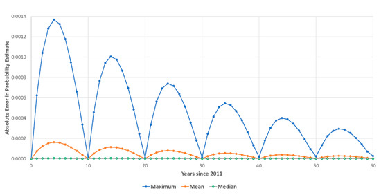
Figure 6.
The error distribution in estimated transition probabilities over all 49 transitions for Florida from 2011 to 2071.
From Figure 6, it is clear that the error declines dramatically as the duration of the time interval increases. Over 60 years, the maximum error dropped from a little over a tenth of a percent at 4 years to less than 3/100 of a percent at 54 years in the last regression sequence. This is logical. While the mathematical proof is beyond the scope of this communication, it can be shown [3,22] that Markov transition matrices contain states that can be characterized as absorbing, transient and recurrent. Absorbing states are those from which it is impossible to escape. In the Florida example, development is an absorbing state. Once a land cover transitions to development, it never transitions to any other class. The transition probabilities for absorbing states remain fixed over time, and thus can be modeled perfectly by the quadratic regression. Transient states are those which transition to either an absorbing state or a recurrent state. Recurrent states are those where a land cover can transition out of a particular class and then return at a later date. A special property of most recurrent states is that they evolve to an equilibrium distribution, with transition probabilities that remain constant over time. As such, they can be modeled perfectly once the equilibrium state is reached. The exception is periodic recurrent states, but these are very unlikely to occur with land cover. Periodic recurrent states require that their persistence transition along the diagonal (such as Forest remaining Forest) has a value of 0 [22]. This is very unlikely, if ever, to occur with land cover, and did not occur in the transition matrices for any of the 48 US states observed. Thus, it is fair to state that land change transition matrices effectively always transition to a limiting stationary matrix where the error associated with the quadratic model of the RBM procedure approaches zero. This then accounts for the progressive reduction in error as the time interval increases.
Another feature that is evident in Figure 6 is that the error at multiples of the base interval (10 years in this illustration), which one would expect to be 0, progressively increases. In the figure, this is only visually noticeable for the maximum error. We believe this is attributable to precision issues as the powering of matrices increases. Both the RBM and TAM procedures are susceptible to this, but it is worse for TAM. For example, to yield the estimate for an interval of 60 years, the RBM procedure only needs to take the base matrix to the power of 6, whereas the TAM procedure needs to take the annualized matrix to the power of 60. Thus, the difference between the two procedures for this component is mostly attributable to TAM. Regardless, the problem is very small (less than 3/1000 of a percent at 60 years).
Finally, it should be emphasized that perhaps the most important feature of the RBM procedure is its simplicity and speed. As noted by [8], the TAM procedure is not feasible for problems with a large number of years and/or land cover classes. For example, our original intent was to use the NLCD data with 15 classes over 10 years. Using the timing information provided by [8], it would take over 43 years to compute each of the annualized transition matrices. For the RBM procedure, it takes less than a second.
6. Conclusions
This study provided a description and evaluation of a Regression-Based Markov (RBM) transition probability matrix estimation procedure for land change modeling and prediction. The problem is to estimate the transition probability matrix necessary to determine the amount of land cover change for any arbitrary time into the future. Unlike a mathematical solution based on eigendecomposition or matrix logarithms/exponentials, which is prone to multiple solutions, frequently involving complex numbers and negative transition probabilities, and even the possibility of no solution, the RBM procedure uses a transition-specific modeling approach that always produces a single non-negative real stochastic matrix.
RBM, however, is an approximation. Comparison with results using eigendecomposition with single stochastic matrices for 42 US states from 2001 to 2011 (which are definitively the correct results), it was determined that the error was typically extremely small (median probability error of 0.00001) and had a maximum error (0.006) similar to that expected from eigendecomposition when a small negative solution is forced to 0 (a common approximation when a single stochastic matrix cannot be achieved). Similarly, comparison with a leading approximation technique in the medical field showed that the RBM algorithm is substantially more accurate, having an error almost five times lower in the worst case encountered.
Error analysis using RBM also showed that errors were at a maximum about 40% of the way between integer multiples of the historical time frame, and decreased to 0 approaching any integer multiple. In addition, as the length of the future projection increased, estimation error of transition probabilies progressively decreased. It was determined that this results from the basic property of Markov transition matrices to evolve to a stable state.
Most importantly, the RBM procedure is capable of finding solutions for large problems with extreme rapidity. A mathematical solution (such as with eigendecomposition) is computationally explosive and effectively infeasible when the number of land cover classes reaches double digits. In contrast, the RBM procedure does not have this limitation and can typically solve in fractions of a second. It thus presents a broadly-applicable approximation with very low error characteristics.
Supplementary Materials
The following are available online at https://www.mdpi.com/2073-445X/9/11/407/s1, Figure S1: Maximum, mean and median error in transition probability estimation for all 49 transitions in Alabama, USA from 2011 to 2021, Figure S2: Maximum, mean and median error in transition probability estimation for all 49 transitions in Arizona, USA from 2011 to 2021, Figure S3: Maximum, mean and median error in transition probability estimation for all 49 transitions in Delaware, USA from 2011 to 2021, Figure S4: Maximum, mean and median error in transition probability estimation for all 49 transitions in Florida, USA from 2011 to 2021.
Author Contributions
Conceptualization, J.R.E. and J.H.; methodology, J.R.E. and J.H.; software, J.R.E.; formal analysis, J.H.; writing—original draft preparation, J.R.E.; writing—review and editing, J.R.E. and J.H.; visualization, J.R.E. and J.H.; supervision, J.R.E.; project administration, J.R.E.; funding acquisition, J.R.E. All authors have read and agreed to the published version of the manuscript.
Funding
This research was conducted as a part of research grant number 4031.02 from the Gordon and Betty Moore Foundation.
Conflicts of Interest
The authors declare no conflict of interest.
References
- National Research Council. Advancing Land Change Modeling: Opportunities and Research Requirements; The National Academies Press: Washington, DC, USA, 2014; ISBN 978-0-309-28833-0. [Google Scholar]
- Olmedo, M.T.C.; Paegelow, M.; Mas, J.F.; Escobar, F. (Eds.) Geomatic Approaches for Modeling Land Change Scenarios; Springer International Publishing: New York, NY, USA, 2017; ISBN 978-3-319-60800-6. [Google Scholar]
- Kemeny, J.G.; Snell, J.L. Finite Markov Chains; Springer: New York, NY, USA, 1976. [Google Scholar]
- Mertens, B.; Lambin, E.F. Land-Cover-Change Trajectories in Southern Cameroon. Ann. Assoc. Am. Geogr. 2000, 90, 467–494. [Google Scholar] [CrossRef]
- Flamenco-Sandoval, A.; Martínez Ramos, M.; Masera, O.R. Assessing implications of land-use and land-cover change dynamics for conservation of a highly diverse tropical rain forest. Biol. Conserv. 2007, 138, 131–145. [Google Scholar] [CrossRef]
- Takada, T.; Miyamoto, A.; Hasegawa, S.F. Derivation of a yearly transition probability matrix for land-use dynamics and its applications. Landsc. Ecol. 2009. [Google Scholar] [CrossRef]
- Chhatwal, J.; Jayasuriya, S.; Elbasha, E.H. Changing Cycle Lengths in State-Transition Models: Challenges and Solutions. Med. Decis. Mak. 2016, 36, 952–964. [Google Scholar] [CrossRef] [PubMed]
- Hasegawa, S.F.; Takada, T. Probability of Deriving a Yearly Transition Probability Matrix for Land-Use Dynamics. Sustainability 2019, 11, 6355. [Google Scholar] [CrossRef]
- Eastman, J.R. TerrSet 2020 Geospatial Monitoring and Modeling System; Clark Labs: Worcester, MA, USA, 2020. [Google Scholar]
- Eastman, J.R.; Toledano, J. A Short Presentation of the Land Change Modeler (LCM). In Geomatic Approaches for Modeling Land Change Scenarios; Camacho Olmedo, M.T., Paegelow, M., Mas, J.-F., Escobar, F., Eds.; Springer International Publishing: New York, NY, USA, 2017; pp. 499–505. ISBN 978-3-319-60800-6. [Google Scholar]
- Mas, J.-F.; Kolb, M.; Paegelow, M.; Camacho Olmedo, M.T.; Houet, T. Inductive pattern-based land use/cover change models: A comparison of four software packages. Environ. Model. Softw. 2014, 51, 94–111. [Google Scholar] [CrossRef]
- Camacho Olmeda, M.T.; Mas, J.F. Markov Chain. In Geomatic Approaches for Modeling Land Change Scenarios; Camacho Olmedo, M.T., Paegelow, M., Mas, J.-F., Escobar, F., Eds.; Springer International Publishing: New York, NY, USA, 2017; ISBN 978-3-319-60800-6. [Google Scholar]
- Camacho Olmedo, M.T.; Pontius, R.G.; Paegelow, M.; Mas, J.-F. Comparison of simulation models in terms of quantity and allocation of land change. Environ. Model. Softw. 2015, 69, 214–221. [Google Scholar] [CrossRef]
- Aung, T.S.; Fischer, T.B.; Buchanan, J. Land use and land cover changes along the China-Myanmar Oil and Gas pipelines – Monitoring infrastructure development in remote conflict-prone regions. PLoS ONE 2020, 15, e0237806. [Google Scholar] [CrossRef] [PubMed]
- Silva, L.P.; Xavier, A.P.C.; da Silva, R.M.; Santos, C.A.G. Modeling land cover change based on an artificial neural network for a semiarid river basin in northeastern Brazil. Glob. Ecol. Conserv. 2020, 21, e00811. [Google Scholar] [CrossRef]
- Lennert, J.; Farkas, J.Z.; Kovács, A.D.; Molnár, A.; Módos, R.; Baka, D.; Kovács, Z. Measuring and Predicting Long-Term Land Cover Changes in the Functional Urban Area of Budapest. Sustainability 2020, 12, 3331. [Google Scholar] [CrossRef]
- Shade, C.; Kremer, P. Predicting Land Use Changes in Philadelphia Following Green Infrastructure Policies. Land 2019, 8, 28. [Google Scholar] [CrossRef]
- Estoque, R.C.; Ooba, M.; Avitabile, V.; Hijioka, Y.; DasGupta, R.; Togawa, T.; Murayama, Y. The future of Southeast Asia’s forests. Nat. Commun. 2019, 10, 1829. [Google Scholar] [CrossRef]
- Kleinbaum, D.G.; Kupper, L.L.; Nizam, A.; Rosenberg, E.S. Applied Regression Analysis and Other Multivariable Methods, 5th ed.; Cengage: Boston, MA, USA, 2014. [Google Scholar]
- Weisstein, E.W. Matrix Power. Available online: https://mathworld.wolfram.com/MatrixPower.html (accessed on 18 August 2020).
- MRLC, Multi-Resolution Land Characteristics (MRLC) Consortium | Multi-Resolution Land Characteristics (MRLC) Consortium. Available online: https://www.mrlc.gov/ (accessed on 31 August 2020).
- Chang, J.T. Stochastic Processes. Available online: https://www.scribd.com/document/206500071/Stochastic-Processes-by-Joseph-T-Chang (accessed on 3 September 2020).
Publisher’s Note: MDPI stays neutral with regard to jurisdictional claims in published maps and institutional affiliations. |
© 2020 by the authors. Licensee MDPI, Basel, Switzerland. This article is an open access article distributed under the terms and conditions of the Creative Commons Attribution (CC BY) license (http://creativecommons.org/licenses/by/4.0/).