Global Open Data Remote Sensing Satellite Missions for Land Monitoring and Conservation: A Review


1
Faculty of Agrobiotechnical Sciences Osijek, Josip Juraj Strossmayer University of Osijek, Vladimira Preloga 1, 31000 Osijek, Croatia
2
Ruđer Bošković Institute, Bijenička 54, 10000 Zagreb, Croatia
3
Faculty of Geodesy, University of Zagreb, Kačićeva 26, 10000 Zagreb, Croatia
*
Author to whom correspondence should be addressed.
Land 2020, 9(11), 402; https://doi.org/10.3390/land9110402
Submission received: 9 October 2020
/
Revised: 21 October 2020
/
Accepted: 22 October 2020
/
Published: 23 October 2020
(This article belongs to the Special Issue Indicators Engineering for Sustainable Land Transformation and Soil Conservation)
Abstract
:The application of global open data remote sensing satellite missions in land monitoring and conservation studies is in the state of rapid growth, ensuring an observation with high spatial and spectral resolution over large areas. The purpose of this study was to provide a review of the most important global open data remote sensing satellite missions, current state-of-the-art processing methods and applications in land monitoring and conservation studies. Multispectral (Landsat, Sentinel-2, and MODIS), radar (Sentinel-1), and digital elevation model missions (SRTM, ASTER) were analyzed, as the most often used global open data satellite missions, according to the number of scientific research articles published in Web of Science database. Processing methods of these missions’ data consisting of image preprocessing, spectral indices, image classification methods, and modelling of terrain topographic parameters were analyzed and demonstrated. Possibilities of their application in land cover, land suitability, vegetation monitoring, and natural disaster management were evaluated, having high potential in broad use worldwide. Availability of free and complementary satellite missions, as well as the open-source software, ensures the basis of effective and sustainable land use management, with the prerequisite of the more extensive knowledge and expertise gathering at a global scale.
1. Introduction
Land conservation strategies arose as a growing necessity in countries worldwide to prevent overexploitation of natural resources and to protect the ecosystem. To satisfy these demands, remote sensing satellite missions became the fundamental data source for land conservation and sustainability globally [1]. The application of remote sensing in land monitoring and conservation is based on the analysis of the reflectance or emittance of individual parts of the electromagnetic spectrum with an observed land cover. Each land cover and its properties result in a unique set of values in the observed parts of the spectrum, being represented by spectral signatures. By analyzing the spectral signatures of the same area observed over different time periods, changes in land cover and its properties are detected. Satellite missions have been one of the main data sources in land monitoring and conservation for many decades, characterized by a wide imaging swath and the ability of integration with various compatible types of imaging sensors [2]. The types of satellite missions differ primarily according to the wavelengths of the electromagnetic spectrum to which sensors mounted on satellites are sensitive. The integration of remote sensing data with the geographical information system (GIS) creates a database of spatial data of the environment, enabling the implementation of spatial analyses for land-use planning [3]. The development of such methods through the use of global satellite missions achieves their applicability in the land monitoring and conservation globally due to the availability of satellite images, which greatly contributes to the popularity of these missions in scientific and professional circles. The development of global open data satellite missions has enabled the wide application of remote land observation, especially for developing countries [4]. Commercial satellite missions are therefore restricted to very high spatial resolution missions and are intended for more specialized land observation, primarily in the monitoring of urban vegetation [5].
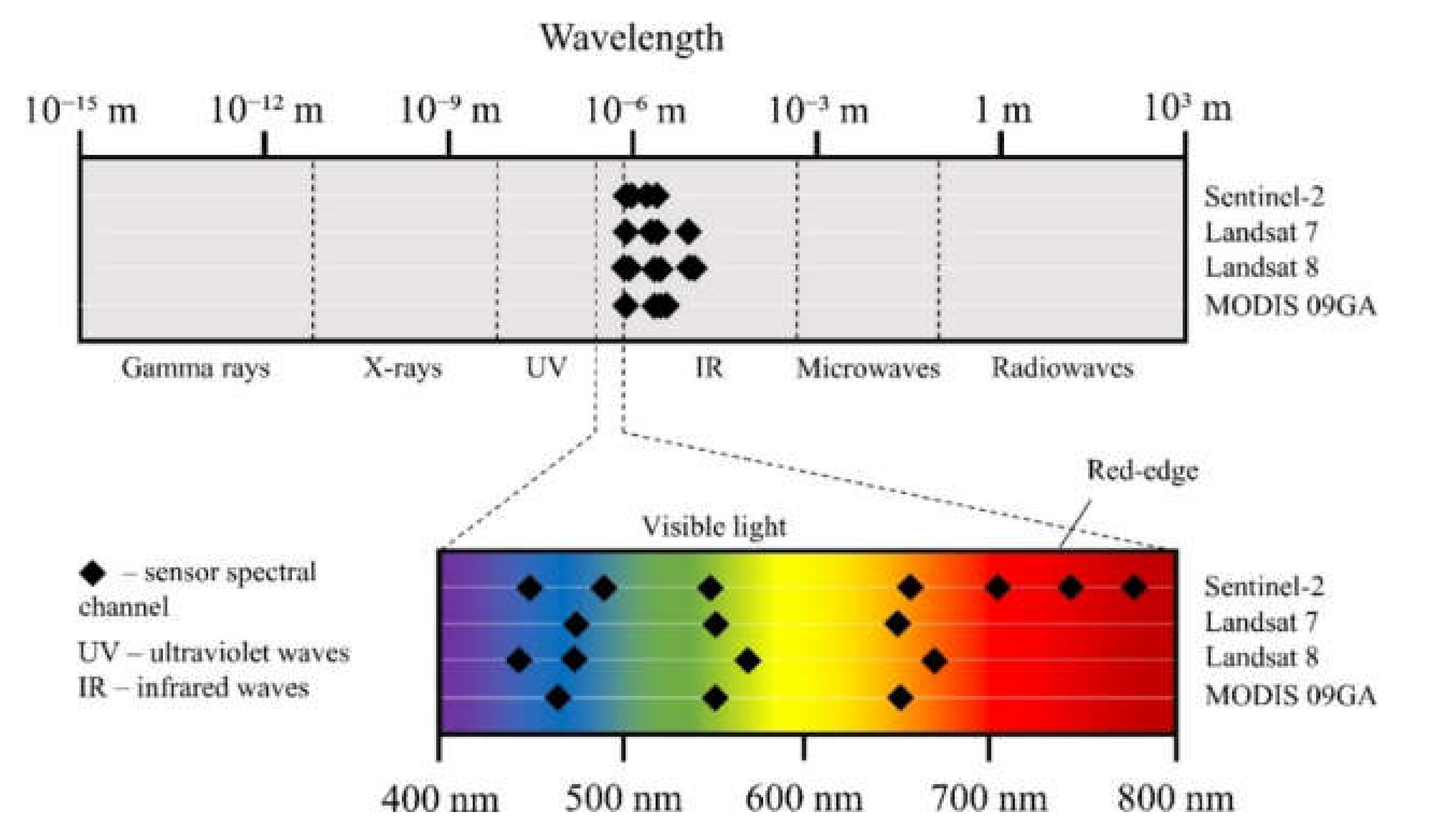
Global open data satellite missions of interest for land monitoring and conservation are primarily multispectral and radar missions, as well as global digital elevation models (DEMs). Hybrid satellite missions have emerged with the development of imaging technology, such as Sentinel-3 owned by the European Space Agency (ESA), which includes a multispectral and radar sensor, in addition to instruments for the ocean and climate monitoring purposes [6]. Hyperspectral and Light Detection and Ranging (LiDAR) sensors have a notable application in land observations, but because of the very high cost they are usually deployed on unmanned aerial vehicles (UAVs) or low-orbit satellites [7]. The operational scope of these systems is currently limited to local scale or is distributed commercially, with high potential for future upgrades and the provision of open data access. The possibility of image fusion of Sentinel-2, Landsat 8, and Moderate Resolution Imaging Spectroradiometer (MODIS) multispectral open data satellite missions allows the analysis of complementary data necessary for land observation [8]. Their spectral sensitivity area regularly covers the visible, near-infrared, and short-wave infrared bands, enabling widespread use in land monitoring and conservation. The red-edge and thermal infrared bands are characteristic of the specific applications of vegetation observations and topsoil temperature [9]. Multispectral images are also compatible with radar images and their fusion allows superior processing accuracy compared to individual sets of satellite images [10].
Web of Science Core Collection (WoSCC) database analysis of the number of articles with the topic of “land” or “landscape” or “environment” refined with the words “remote sensing” from 2010 to 2019 confirmed the observation of the widespread use of global open data satellite missions in land monitoring and conservation studies (Figure 1). Open data missions recently gained popularity compared to commercial satellite missions, with the 6.2 times more land-related studies based on using open data remote sensing missions being published in 2010 and 11.5 times in 2019. Among the open data global satellite missions, MODIS is traditionally represented in land monitoring and conservation studies, with the recent increase of moderate spatial resolution missions’ application, primarily Sentinel-2 and Landsat 8. The application of all three current ESA Sentinel missions is rapidly growing for the land and environmental research. An increase of 396%, 371%, and 281% for the application of Sentinel-1, Sentinel-2, and Sentinel-3 data, respectively, were noted between 2017 and 2019 based on the WoSCC database. Global DEMs, Shuttle Radar Topography Mission (SRTM), and Advanced Spaceborne Thermal Emission and Reflection Radiometer (ASTER), were steadily used in land monitoring and conservation studies since their start of operability.
Land conservation is an important part of worldwide sustainability strategies, with the focus on the conservation of natural landscapes, as well as anthropogenic ecosystems, especially in the European Union (EU) [11]. EU Biodiversity Strategy for 2030 noted land-use changes as one of five drivers of biodiversity loss, whose monitoring allows conservation of plant and animal species [12]. According to the same source, land cover changes caused expenses up to €29 trillion globally due to the effects of land degradation and ecosystem services in the 15-year period. The necessity of land monitoring and conservation is addressed in the Republic of Croatia as a necessity due to growing urbanization [13], with remote sensing data being one of the fundamental data sources for land use management. The National Strategy of Environment Protection of the Republic of Croatia, underlines the importance of satellite remote sensing in the GIS environment, being essential for land conservation and sustainable development [14]. Due to the possibility of remote observation of an inaccessible and potentially dangerous area, the remote sensing is complemented by conventional field observation methods of soil, water, and atmosphere. The most recent report on the state of the environment in the Republic of Croatia for the period from 2013 to 2016 noted the particular importance of multitemporal satellite images and their analysis in the GIS environment for monitoring changes in land cover, especially for the monitoring of vegetation properties [15]. Satellite mission data in the same document are classified in the category of primary data sources, which form the basis of the analysis of environmental indicators and future reports.
The aim of this paper was to analyze the most commonly used global open data satellite missions, data processing methods and their application in land monitoring and conservation. The primary segment of their importance is accessibility to the broad scientific community for the application in land conservation studies and strategies. Further development of these missions and familiarization with their possibilities provides the basis for the upgrade of land monitoring services and their widespread use globally.
2. Global Open Data Remote Sensing Satellite Missions
The global open data remote sensing satellite missions are analyzed according to the classification to multispectral missions, radar missions, and DEM acquiring. Major missions per classification were highlighted according to their popularity in articles for land monitoring and conservation using remote sensing indexed in WoSCC database in the last ten years (2010–2019). All representative figures in the paper were created by the authors, based on the freely available global open data satellite mission imagery.
2.1. Multispectral Satellite Missions
Remote sensing using multispectral sensors is performed by registering incoming reflected or emitted energy from objects on the earth’s surface, which is dispersed and registered in sensors sensitive to certain spectral bands [16]. These spectral bands are represented as a narrow part of the electromagnetic spectrum, defined by the smallest and largest wavelength of the sensor sensitivity, which results in one raster image per spectral band. Spectral bands of four most commonly used global open data multispectral satellite missions are displayed in Figure 2, where black squares represent their spectral coverage in visible, red-edge, and infrared parts of the spectrum. The intensity of the incoming energy on the sensor is converted to digital numbers, which also depend on atmospheric conditions at the sensing time. As a result, the numerical value shows the relative relationship of reflection at the time of observation and does not represent a measurable physical unit [17]. For the quantitative interpretation of such data, it is necessary to perform the conversion of numerical values into reflectance, or the ratio of the amount of reflected energy per spectral band and the total incoming energy at the sensor. Detection and identification of land cover and its properties are based on differences of spectral signatures per spectral band. Each specific property of land cover results in unique spectral signatures, with a noticeable difference in its reflectance in one or more spectral bands compared to the rest of the observed area [18]. By highlighting these differences using the processing methods described in the next chapter, these characteristics are quantified or extracted from the rest of the observed area, which serves as a basis for interpretation and decision-making in land conservation.
Sentinel-2 is a multispectral satellite mission with moderate spatial resolution within the ESA Copernicus program. The main purpose of the mission is the observation of the Earth’s surface to provide forest and vegetation monitoring services, detection of land cover changes and management of natural disasters [19]. The imaging is performed using a Multispectral Imager (MSI) instrument mounted on two satellites, Sentinel-2A, and Sentinel-2B. The satellites are polar-orbiting on diametrically opposite sides of the same sun-synchronous orbit, allowing the observation of the Earth’s surface between 84° N and 56° S latitudes.
The Landsat 8 satellite mission, owned by the National Aeronautics and Space Administration (NASA), uses two multispectral sensors, the Operational Land Imager (OLI) and the Thermal Infrared Sensor (TIRS). OLI uses nine spectral bands in the visible, near-infrared, and short-wave infrared part of the spectrum for moderate spatial resolution observations, while TIRS complements multispectral observation with two thermal bands with a lower spatial resolution [20]. Landsat 8 is an upgrade to the previous mission of the same series, Landsat 7, through better spectral resolution and a rectified error in observing the edge parts of the imaging area.
MODIS is a multispectral satellite mission owned by NASA and named after a multispectral sensor mounted on two satellites, Terra and Aqua, orbiting on diametrically opposite sides of the same polar orbit. MODIS is intended for remote sensing of land, oceans, and lower atmosphere, enabling high temporal resolution and a very wide imaging swath [21]. Due to the complexity and diversity of MODIS products, MODIS09GA data were selected as a representative product regarding average spatial and spectral resolution in relation to other MODIS products.
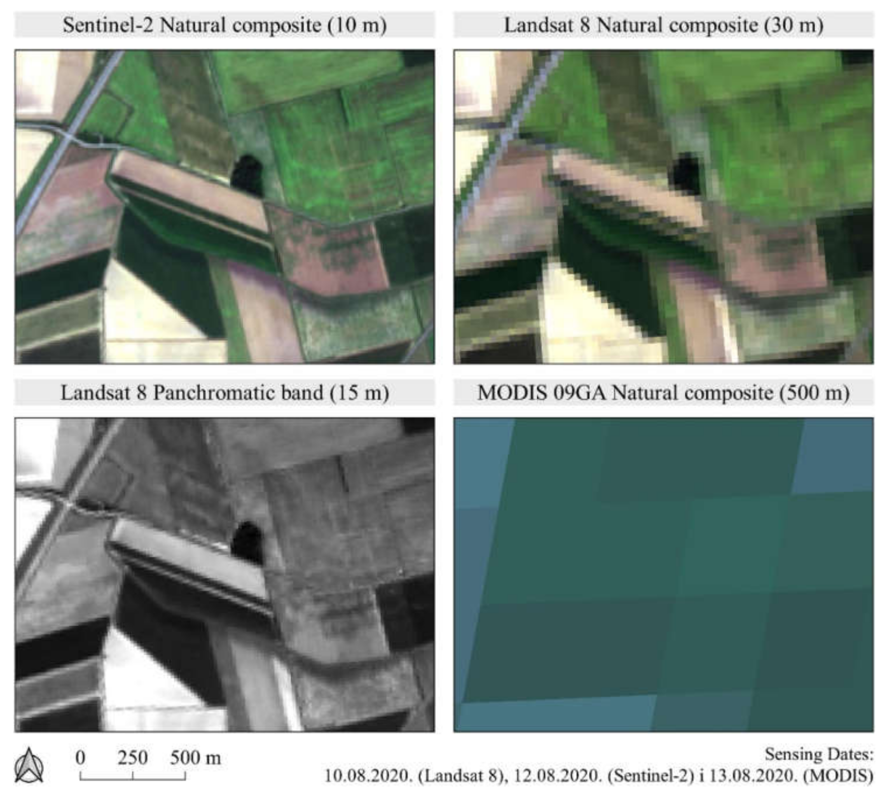
The basic characteristics of the most commonly used satellite multispectral missions applied in environmental studies are presented in Table 1. The supported research area is classified according to the classification by Herod [22], arranged from smaller to larger in a local, national, regional, and global scale. The greatest impact for this classification was the spatial resolutions of each mission, which are comparatively represented in Figure 3. Landsat missions contain a panchromatic band of 15 m spatial resolution, which serves as the basis for pan-sharpening of other images in the visible and near-infrared part of the spectrum to 15 m spatial resolution while preserving spectral values. The same procedure is possible by applying a 10 m spatial resolution visible light bands of Sentinel-2 for pan-sharpening of the red-edge and near-infrared images [23].
2.2. Radar Satellite Missions
Microwave sensors, commonly known as radars, belong to a group of active sensors. The method of registering the intensity of reflected energy by radars depends on the radar system’s properties and terrain characteristics, primarily surface roughness and water content in soil and vegetation [24]. The specific characteristics of each radar system in remote sensing are the polarization of the electromagnetic waves, the angle of energy transmittance and its wavelength [25]. Polarization of the emitted or reflected electromagnetic wave represents the orientation of the electric field at the time of transmission or registration, which may be horizontal (H) or vertical (V). If the radar is sensitive to both polarizations, one or more images of different combinations of transmitted and registered polarizations in combinations of HH, HV, VH, or VV are created. Due to the differences in the registration of reflected polarization, these images contain different, most commonly complementary information of land cover and its properties [26].
Sentinel-1 is a radar satellite mission, the first of six planned missions within the ESA Copernicus program. It consists of two Sentinel-1 satellites carrying a synthetic aperture radar (SAR) and orbiting on diametrically opposite sides of the same polar orbit, resulting in a temporal resolution of six days [27]. This SAR is sensitive to wavelengths in the C-band of the electromagnetic spectrum, which covers wavelengths ranging from 3.8 to 7.5 cm. The advantage of remote sensing using radar is the ability of observation regardless of atmospheric conditions, as microwaves pass through fog, rain, and clouds [28]. The radar images at the pre-processing Level-1 available for download contain raw SAR observation data which were previously internally calibrated to the mean signal frequency using the Doppler centroid method. Radar imaging is performed by single or double polarization, which results in a spatial resolution in range of 10 and 40 m. The basic two products of Sentinel-1 are single look complex (SLC) and ground range detected (GRD) images [27]. SLC images consist of directed SAR data containing the complete phase and related complex data. These images are georeferenced using the data of the satellite orbits and positions at the sensing time, corrected for oblique observations of the terrain. GRD images contain generalized directed SAR data, projected in the WGS84/UTM projection coordinate system using an ellipsoid model. These images contain pixels with approximately square shape and reduced noise, but with a lower spatial resolution than SLC images. Phase data is therefore lost, but GRD images take up to five times less hard disk memory than SLC images.
2.3. Digital Elevation Models
The DEMs from global satellite missions contain absolute elevation as pixel values in raster data, indicating the average elevation in the observed area. Two basic methods of DEM calculation using satellite missions are based on the radar interferometry and image stereo pairs. The two most widely used global digital height models are the SRTM and the ASTER owned by NASA, according to the number of published land monitoring and conservation research articles in WoSCC in the last decade. SRTM contains elevation data with a spatial resolution of approximately 30 m, which is currently the highest spatial resolution of global open data DEMs.
SRTM is a global satellite mission for radar imaging of the Earth’s surface used to calculate the global set of digital elevation data. The observations were performed in the range of 60° N to 56° S latitudes [29]. The basic principle of data collection and processing is radar interferometry, based on the comparison of two radar images of the same area sensed at different angles. ASTER is also a global satellite mission with the goal of DEM calculation, named after an instrument mounted on the Terra satellite. To create a DEM, remote sensing was performed in the near-infrared spectral band and processed by the image stereo pairs analysis method [30]. An additional property of the ASTER mission is the corrections for the elevation values of water surfaces, whereby the seas and oceans are characterized by uniform elevation, while rivers were modelled by proportionally lower elevations downstream.
3. Methods of Processing and Analyzing Remotely Sensed Data
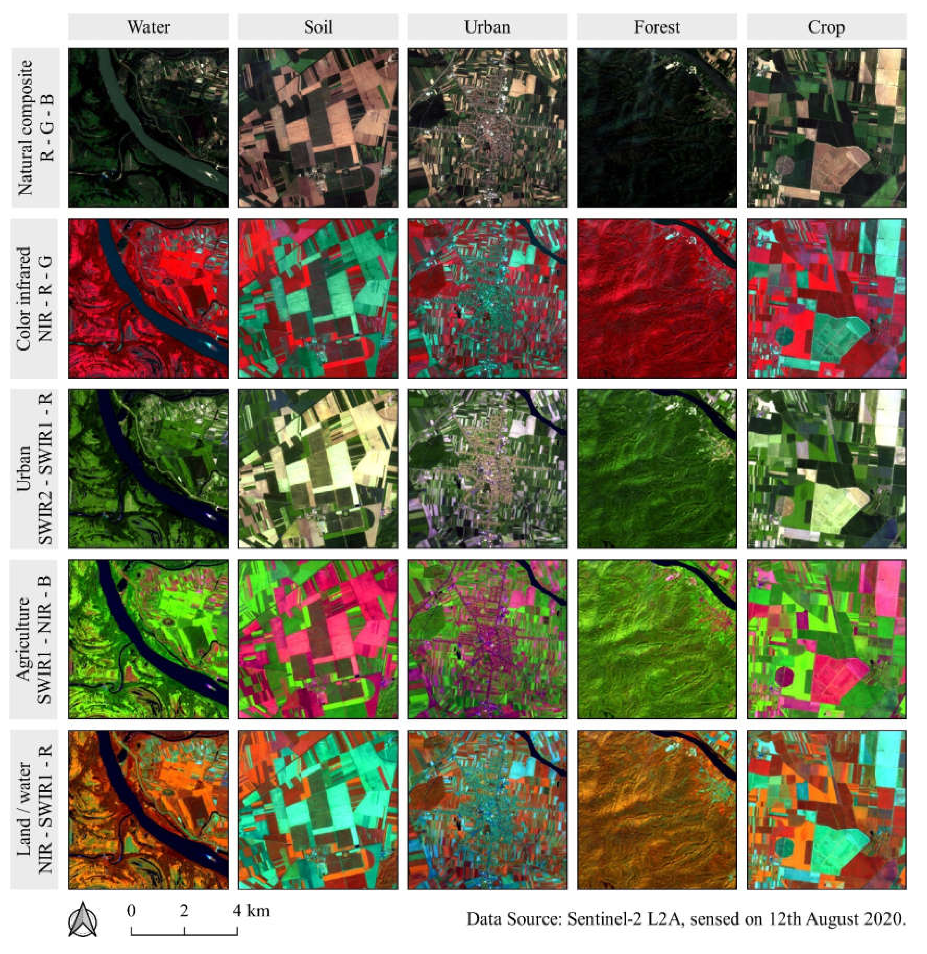
The processing and analysis of data collected by one of the previously described satellite missions can generally be divided into three directions: visual, quantitative, and qualitative. A prerequisite for processing and analyzing with any approach is the image pre-processing [31]. It represents a set of corrections for remotely sensed data, which is specific for each individual satellite mission. The visual analysis method is the simplest and relatively limited approach for the interpretation of remotely sensed data. It is commonly applied in terrain reconnaissance and the identification of generalized land cover classes [32]. The visual interpretation is applicable for multispectral images using RGB composites, where it is possible to display terrain characteristics specific for the selected combination of spectral bands. The RGB composites based on Sentinel-2 images for specialized purposes in visual analysis are displayed in Figure 4. All used spectral bands were resampled to 20 m spatial resolution prior to the creation of RGB composites.
The quantitative approach is dominantly based on the application of multispectral images, by combining pixel values of several different spectral bands. The selected property of the observed area is quantified by the application of spectral indices, where the values of that property are proportional to the values of the calculated spectral index [33]. Mathematical models for modelling of the topographic terrain parameters based on the DEM also quantitatively evaluate the calculated properties. Qualitative evaluation of the terrain is based on the classification of spectral values of image pixels or objects in the predefined number of classes. This approach is flexible in terms of selecting spectral values as an input in the classification and does not necessarily require calibration of remotely observed values to physical units, but rather implements the relative classification of parts of the observed area. Open source GIS software, SAGA GIS v7.4.0 and QGIS v3.8.3, were used for data processing in case studies of global open data satellite missions in the next subsections.
3.1. Image Pre-Processing
The basic pre-processing procedures of any data obtained by remote sensing are the transformation into a selected coordinate reference system and grid clipping to an area of interest. Remote sensing data of the missions described above are commonly distributed in WGS84 or WGS84/UTM projection coordinate systems worldwide.
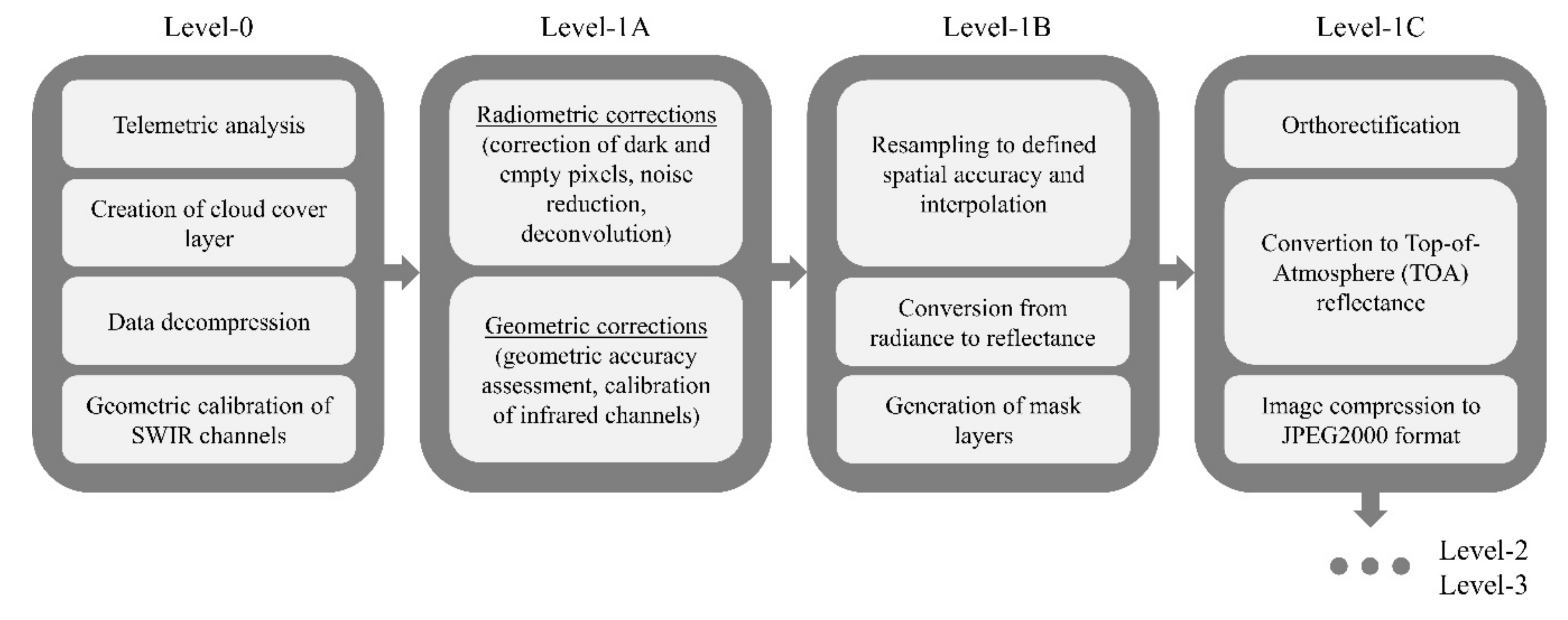
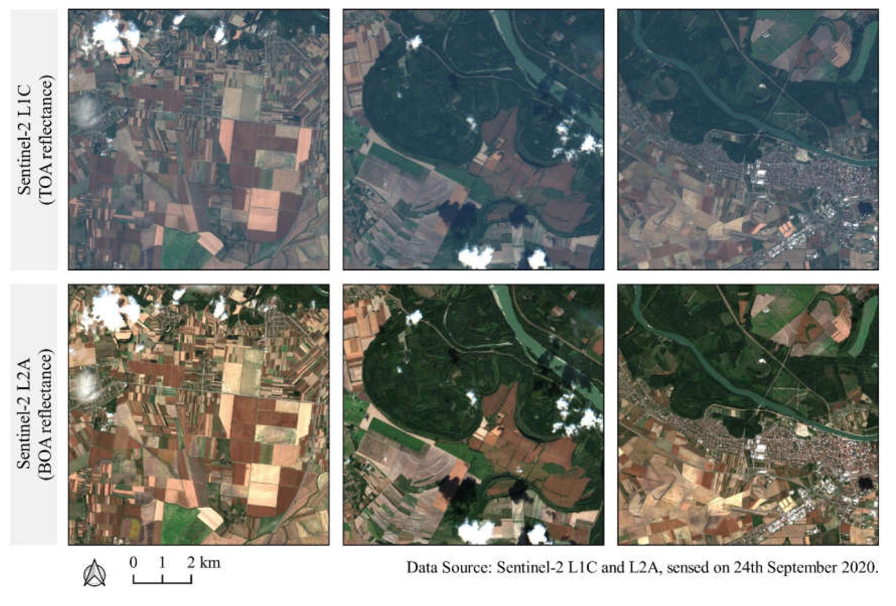
Multispectral images of Sentinel-2, Landsat and MODIS missions are mostly available to users at level 1C pre-processing and contain orthorectified data with geometrically calibrated reflectance values at the top of atmosphere (TOA). Data at earlier pre-processing levels is not openly distributed to users and is performed by organizations managing the satellite mission. Pre-processing corrections for Sentinel-2 satellite images performed by the ESA are displayed in Figure 5. Using the atmospheric corrections, users have the possibility of independent conversion of TOA reflectance to the bottom of the atmosphere (BOA) reflectance, which corresponds to the 2A pre-processing level. This eliminates the influence of atmospheric factors on reflectance at the sensing time, which makes is available for quantitative processing and analysis of the observed area. A comparative display of Sentinel-2 RGB natural composites based on TOA reflectance from Level-1C data and BOA reflectance from Level-2A data is shown in Figure 6. Some satellite missions, primarily Sentinel-2 and Landsat 8, have enabled free downloading of Level-2A images in recent years, with the conversion to the BOA reflection coefficient carried out by data distributors. Further Level-2 and Level-3 data designate more complex remote sensing products, such as land cover classification.
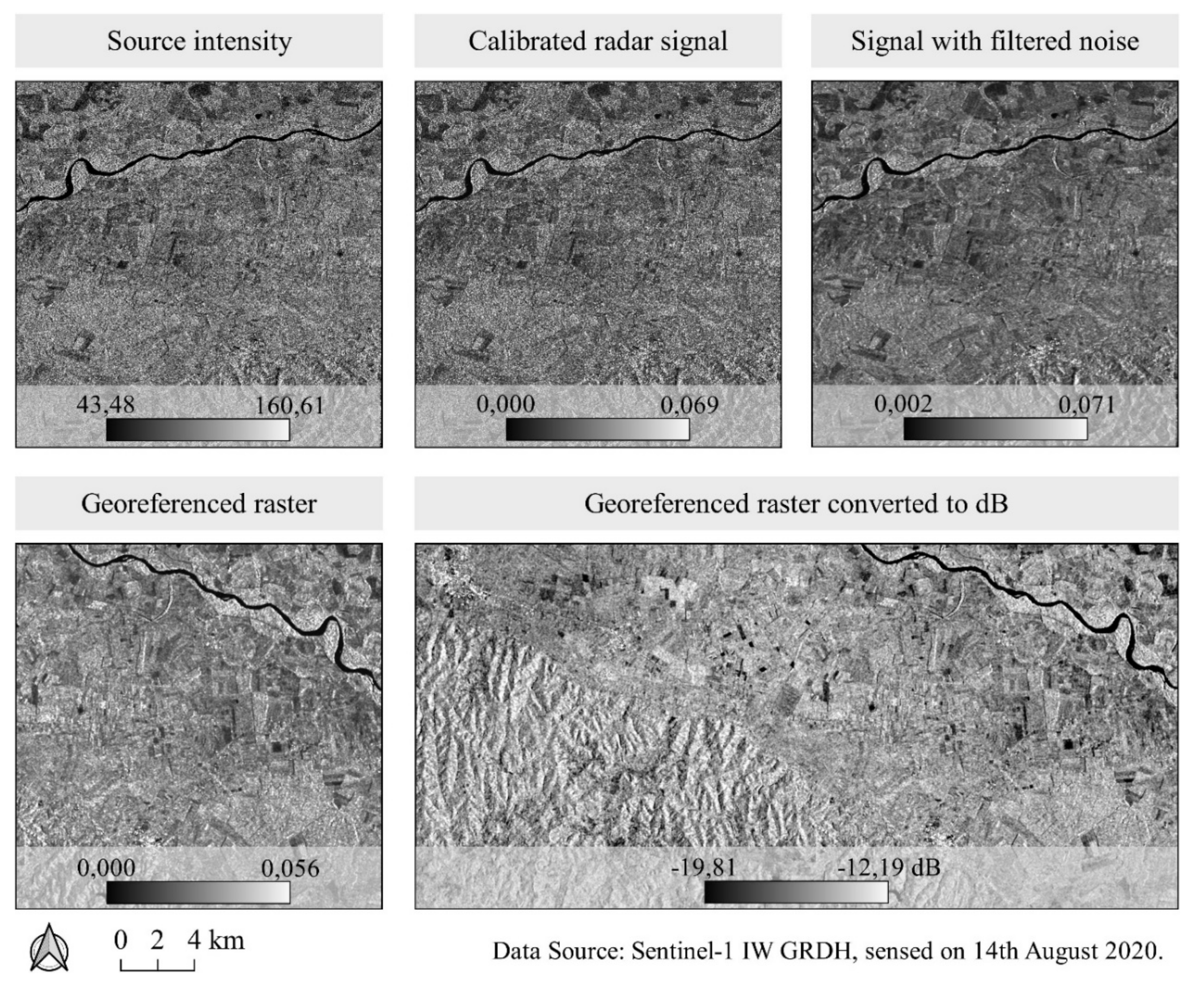
The pre-processing of radar images consists of four basic steps: radiometric correction, signal noise filtering, geometric correction, and georeferencing, conversion of registered signal intensity value to decibels (dB) (Figure 7) [34]. Radiometric calibration results in the conversion of the originally registered intensity to absolute normalized radar backscatter intensity using coefficients from the image metadata. Filtering or radar images reduces the amount of noise on the images, caused by coherent processing of return radar signals from multiple different surfaces on the ground within a single pixel. Frequently used filters are speckle filters, which smooth the image by calculating the mean pixel value from the selected pixel matrix [35]. Selecting a larger filtering pixel matrix proportionally reduces noise and spatial resolution of the image. For the pre-processing of the images displayed in Figure 7, the Lee Sigma filter with a matrix of 7 × 7 pixels was applied. Geometric correction eliminates the influence of relief and angle of radar observation on image values using orthorectification [36]. During the georeferencing process, the radar images are transformed into the correct position in the selected coordinate reference system. Doppler’s orthorectification method of SAR images into the Croatian Terrestrial Reference System (HTRS96/TM) was also performed, using a global SRTM 1-arc second DEM for the orthorectification.
The pre-processing specific for hydrological analysis of the terrain using a DEM is a mathematical filling of depressions, on which it is not possible to determine the direction of water flow. This correction is usually carried out by the Fill Sinks method, where it is necessary to define the value of the slope tolerance of the elevation filling [37].
3.2. Spectral Indices
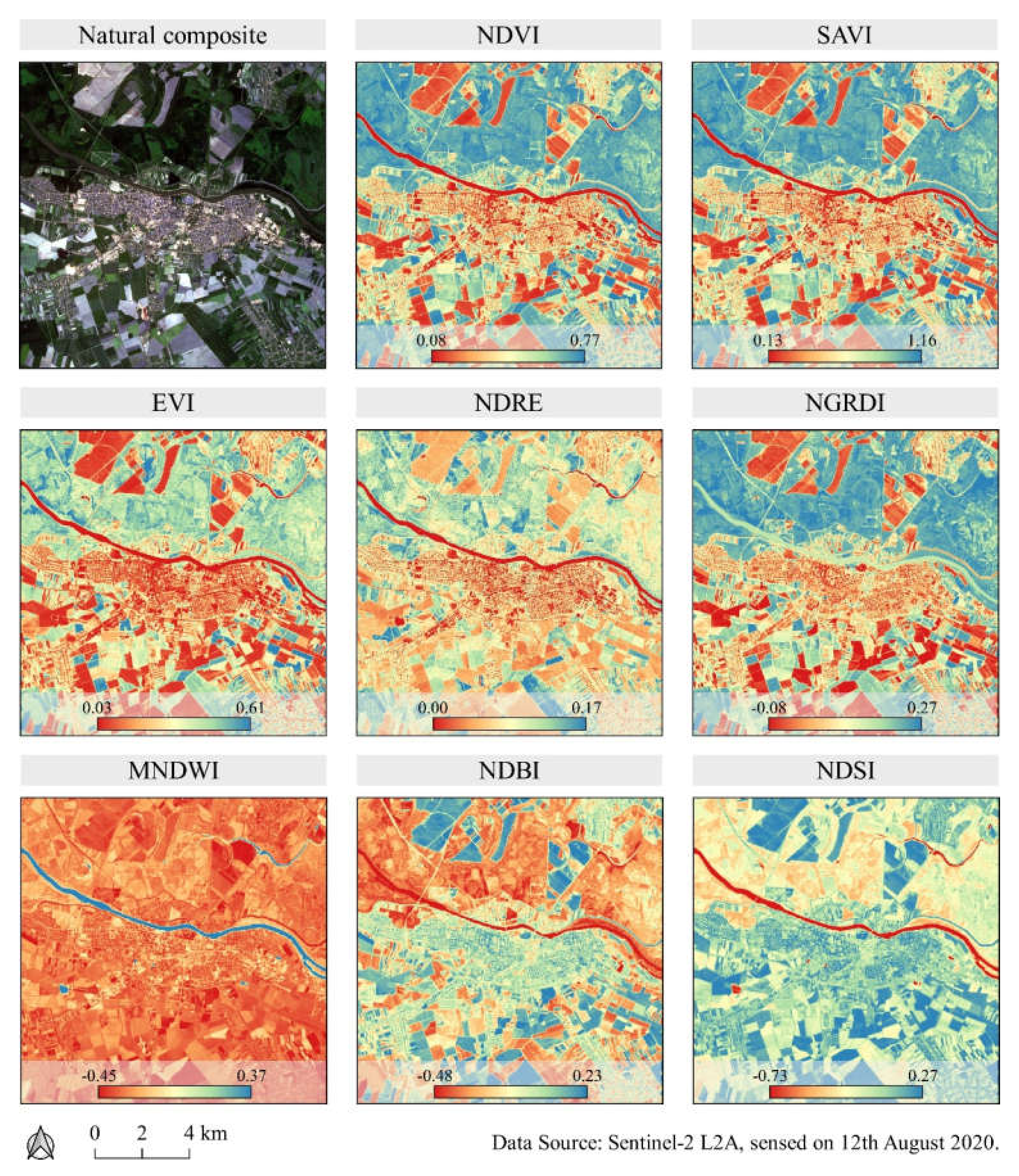
Spectral indices are calculated using arithmetic functions of pixel values from two or more remotely sensed spectral bands (Table 2; Figure 8). Each spectral index aims to extract a certain type of land cover or its specific property, which is characterized by distinct values relative to the rest of the observed area. Spectral indices are often calculated using normalized differences of reflectance in two spectral bands, with the highest and lowest sensed relative reflectance of a particular land cover property. The advantage of this approach is the known possible range of spectral index values at interval (–1, 1), which makes it possible to achieve repeatability of the values of specific land cover property and therefore monitoring its changes in time.
Spectral indices whose primary purpose is to enable monitoring of vegetation properties are known as vegetation indices. Their quantity and the range of applications in environmental monitoring are the widest of all spectral indices, as there are currently about 250 unique vegetation indices that can be calculated using Sentinel-2 satellite images [46]. Some of the most commonly used vegetation indices are the normalized difference vegetation index (NDVI), soil-adjusted vegetation index (SAVI), enhanced vegetation index (EVI), normalized difference red edge (NDRE), and normalized green-red vegetation index (NGRDI). The calculation of vegetation indices is based on the emphasis of the difference in the vegetation reflectance from very low in red, to very high in the near-infrared or red-edge spectral bands. With the application of low-cost RGB cameras, which offer the possibility of remote sensing only in the visible part of the spectrum, a green band is often used as an alternative to the red-edge or near-infrared band [47]. Almost all vegetation indices have the same primary purpose, but each is specific regarding highlighting certain vegetation properties or noise reduction due to reflectiveness of the bare soil. Although NDVI is the world’s most widely used vegetation index for a wide range of applications in the monitoring of vegetation properties [48], it has a limitation in the form of low sensitivity to minor differences in case of high chlorophyll content and biomass, known as the saturation effect [49]. In this case, NDRE provides the alternative due to the greater sensitivity of the red-edge band to these vegetation properties [50]. Due to mutual compatibility, NDVI and NDRE are often used for the remote sensing of agricultural crops by applying sensors on agricultural machinery during precise fertilization and crop protection. The SAVI uses a correction factor to reduce the influence of bare soil reflectance, while a blue band for the calculation of EVI is used to reduce the influence of atmospheric effects during remote sensing [51]. The secondary purpose of vegetation indices is to extract areas under vegetation from the soil and artificial land covers due to their sensitivity to the chlorophyll content and biomass. For this reason, they are often used in combination with other processing methods of remote sensing data, resulting in high processing efficiency and high accuracy of land observation models [47]. Modified normalized difference water index (MNDWI) is used as a complement to vegetation indices when monitoring vegetation since it is sensitive to water content in vegetation and soil. It is a modified version of another commonly used spectral index, normalized difference water index (NDWI), which was upgraded by reducing noise of the detection of soil and vegetation water content by using green, instead of near-infrared spectral band [43]. MNDWI is also applied for land cover mapping, as it achieves maximum values for water surfaces. Normalized difference built-up index (NDBI) and normalized difference soil index (NDSI) are used primarily in monitoring of land cover changes for built-up objects and soil and their distinction, as these land cover classes often have similar spectral signatures.
3.3. Image Classification
The classification methods in remote sensing are based on the classification of the fundamental image parts into a predefined number of classes. Classification is often an indispensable procedure in the remote sensing for land monitoring and conservation, as it allows determination of land cover classes and its properties with high accuracy over a large area [52]. The necessity for manual field observation is consequentially decreased to discrete locations, used as a test dataset for the accuracy assessment of classification results. The fundamental image parts in classification are either pixels or objects, defined as two or more neighboring pixels of similar spectral and textural properties. These parts are classified in the n-dimensional space, where n represents the number of input grids in the classification. Input grids in the classification are the most commonly original images and spectral indices. Various spectral indices, like NDVI, NDBI, and MNDWI, were successfully integrated with the classification using Landsat 7 and Landsat 8 images by Estoque and Murayama [53]. The object-oriented classification is the superior classification approach, with the advantage of lower noise in classification results caused by atmospheric effects, as well as a more generalized result that accurately represents the actual situation in the field than pixel-based classification [47].
Classification in the number of classes defined by the operator can be performed either without the training dataset (unsupervised classification) or by determining the training dataset for individual classes of selected land cover properties (supervised classification). Training datasets contain representative samples of each defined class in form of groups of pixels or objects, created based on field observations or visual identification on the images. Unsupervised classification algorithms are based on the iterative classification of the fundamental image parts into a defined number of classes according to a defined non-parametric criterion [54]. The most commonly used unsupervised classification algorithms are k-means, which is based on the minimum Euclid distance of spectral values to the center of the class and the iterative uniform adjustment of the class center and ISODATA, which similarly adjusts the centers of classes based on the criterion of the least distance to the center of the class. Conventional supervised classification algorithms operate on a similar principle, but class centers are defined by spectral values of the training dataset and are not subject to iterative adjustment to input data. The main property of this approach is the subjectivity of the operator, which results in its greater influence on the classification process due to the possibility of arbitrary formation of class centers in the n-dimensional system of input values. This can result in multiple classes of close spectral values, which often correspond to the actual conditions in the field. For an independent accuracy assessment of the classification results by supervised classification, the creation of a ground-truth dataset containing representative class samples using field identification or vectorization based on visual identification of images is common. This unique dataset is then randomly divided into training and test datasets in ratios of 30:70 or 20:80, resulting in the reduced operator’s subjectivity during the classification process.
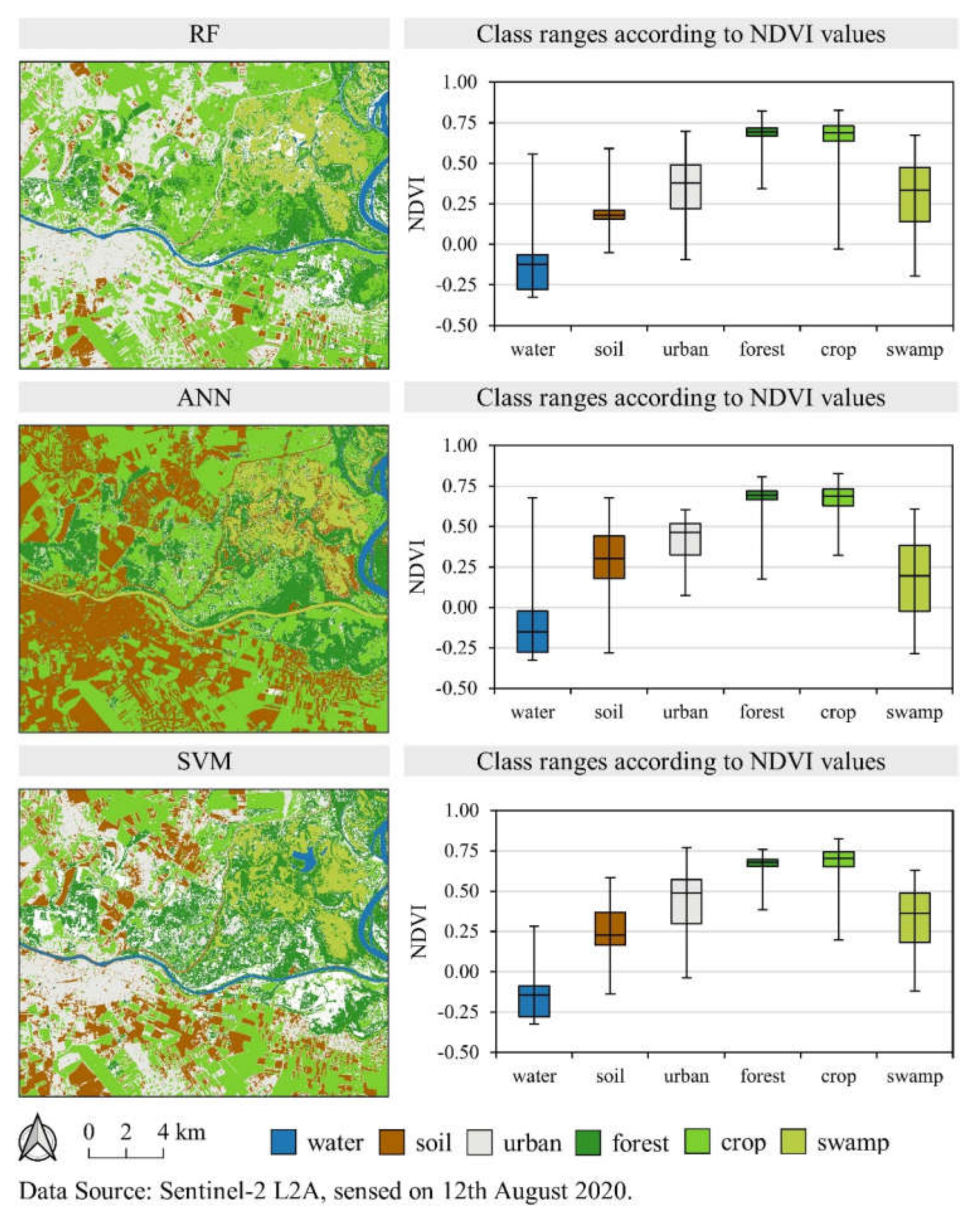
Some of the conventional algorithms of supervised classification are maximum likelihood and minimum distance to mean. Over the past decade, machine learning algorithms have completely replaced conventional algorithms of supervised classification from application in land monitoring and conservation. The superior accuracy of classification results, reduced overfitting and computing efficiency are the main advantages of machine learning algorithms over conventional supervised classification algorithms [55]. The most commonly used machine learning algorithms for supervised classification in remote sensing currently are random forest (RF) [56], artificial neural networks (ANN) [57] and support vector machines (SVM) [58]. The performance of these algorithms is visible in Figure 9, which contains the classification results calculated using the same training dataset on Sentinel-2 images. Resulting classes were represented according to boxplots containing NDVI values, as the values of spectral indices commonly differ with land cover classes [59].
The current trend of machine learning algorithms development in remote sensing are deep machine learning algorithms [60]. Their advantage over the machine learning algorithms described above is the higher classification accuracy and processing capabilities of a larger quantity of training samples, but their characteristics and performance still require additional research. The implementation of these algorithms requires expensive computer hardware, primarily in terms of the graphics processing unit (GPU), which currently makes them less available for use in a broad scientific community.
3.4. Modelling of Terrain Topographic Parameters
Modelling of terrain topographic parameters is based on using a DEM, according to the neighborhood values of individual pixels, as well as the latitude of the specific location. Calculated models represent theoretical values and approximation of actual conditions in the field at the micro-level. The significance of such models is in the relative relationship of calculated values, which for spatial planning and suitability analyses allows adequate representation of the terrain topography. Figure 10 displays various terrain topographic models calculated using SRTM DEM: slope [61], wind exposition index, potential incoming solar irradiation [62], flow accumulation model [63], and topographic openness [64]. Terrain slope is the basic topographical parameter of the terrain and is widely used in spatial planning in civil engineering, transport, and environmental studies [65]. Potential solar irradiation was calculated for the year 2020, using a 70% generalized atmospheric permeability parameter, which includes the influences of clouds, fog, and precipitation on the amount of incoming solar radiation. The wind exposure index is calculated by analyzing the individual elevations of pixels and adjacent pixels incrementally every 15°, covering the entire horizon around a pixel of 360°. The baseline value for the flat area is 1, with lower values proportionally indicating more covered areas, while higher values indicate a more exposed area to wind. The flow accumulation model was calculated using the top-down method and the multiple flow direction technique, gradually analyzing the relative elevation difference of individual pixels, starting with those with the highest elevation value. For each pixel, eight neighboring pixels were observed, and the final values of the flow accumulation model represent the total surface from which precipitation or water potentially flows from higher elevations. This model represents a single component of the hydrographic analysis of the terrain, as precipitation drainage and water flow depend on several factors, such as land cover class or soil texture [66]. The topographic openness index indicates the horizon exposure for a single pixel, which is applicable for spatial planning in the construction and analysis of animal and plant habitats.
4. Applications of Land Monitoring and Conservation Using Satellite Missions
The application of global open data satellite missions covers a wide range of possibilities, most commonly for monitoring of land cover and vegetation changes, environmental and natural disasters, as well as the land suitability calculation using GIS-based multicriteria analysis. The development of new satellite missions is also expected to improve existing atmospheric and ocean monitoring systems.
4.1. Land Cover Change Monitoring
The observation of land cover changes over a period of time is one of the fundamental sources of information in land conservation. The classification of the observed area into several generalized land cover classes creates a universal basis for spatial planning and monitoring of changes in the environment. Some of the most important environmental factors, such as climate change, deforestation, and urbanization, are determined by comparing land cover databases created for two or more different time periods [67]. The same data are used to quantify biodiversity and detect endangered areas due to deforestation or various socio-economic reasons [68]. Global satellite missions, especially multispectral missions, are the most common source of data for the classification of land cover due to the high temporal resolution and the suitability for efficient computer processing [69]. For the monitoring of land cover changes, standardization of land cover classes over different time periods is necessary for their mutual comparison [70]. The most commonly used land cover classes within the EU are artificial (urban) areas, agricultural areas, forests, wetlands, and water bodies, according to the Corine Land Cover (CLC) classification within the ESA Copernicus program. The latest version of the land cover database in the EU, CLC 2018, was produced using the Sentinel-2 and Landsat 8 multispectral images with thematic accuracy above 85% [71]. For specialized studies and applications in environment monitoring, an additional classification of generalized classes in multiple subclasses is performed. For example, the agricultural areas class is divided into four subclasses in the CLC 2018: arable land, permanent plantations, pastures, and heterogeneous agricultural land, and a further 11 subclasses at the third level [71]. Algorithms of supervised machine learning classification are currently a fundamental method of processing satellite images for the land cover classification [72], and more frequent application of deep machine learning algorithms for the same purpose is expected in the future [73]. Trends in the development of classification algorithms of land cover from satellite images are also directed to their automation, thus reducing the processing time, and eliminating the possibility of operator subjective error in determining the training dataset for classification [74].
4.2. Land Suitability Determination Studies Using GIS-Based Multicriteria Analysis
The GIS-based multicriteria analysis is a fundamental approach to the creation of land suitability studies, characterized by a high level of flexibility and computational efficiency. The premise for the implementation of multicriteria analysis is the spatial component of the study objective and the criteria on which land suitability depends. The suitability calculation of environmental factors using GIS multicriteria analysis generally consists of six basic procedures [75,76]:
- Definition of the study aim
- Selection of spatially related criteria affecting the land suitability
- Standardization of criteria values
- Determination of criteria weights
- Calculation of land suitability by combining standardized values and criteria weights
- Accuracy assessment and interpretation of results
The application of GIS multicriteria analysis in land conservation is based on the optimal utilization of existing natural resources and the preservation of their quality and quantity. The objectives of GIS multicriteria analysis in land conservation are often based on multidisciplinary sciences, covering sustainable waste management, agricultural production planning, groundwater protection, natural disaster risk mapping and spatial planning of energy plants. Two main objectives in sustainable waste management are the suitability analyses of the existing and planned landfills [77], as well as the suitability of waste incinerator locations [78]. The appropriate waste management method, especially in urban environments, reduces air, water and soil pollution caused by the discharge of ammonia, heavy metals, and nitrates from waste [79]. The application of GIS-based multicriteria analysis in agriculture focuses on the calculation of cropland suitability according to climatic, pedological, and topographical terrain conditions [65]. The selection of the optimal area for crop cultivation reduces the need for the application of fertilizer and pesticides, resulting in a lower release of heavy metal contaminants into the environment. Groundwater is the most important natural resource for the global water supply [80]. Using GIS-based multicriteria analysis, zoning of groundwater properties is indirectly performed by several indicators affecting groundwater status, such as climatic, topographic, and geological criteria, as well as certain soil properties, such as drainage [81]. Natural disasters risk mapping using GIS-based multicriteria analysis enables the development of an emergency plan for forest wildfires, floods, and other disasters. The multiannual climate and hydrological criteria in such analyses provide the basis for the insurance of crops due to damage caused by hail or drought [82]. Construction planning of costly and environmentally-friendly power plants is based on the existing renewable energy sources and natural habitats, spatially modelled using satellite mission data. The GIS-based multicriteria analysis is one of the fundamental procedures for the energy plants construction according to land conservation requirements, such as for solar power plants [83] and windmills [84]. Criteria modelled using satellite missions used in GIS-based multicriteria analyses for the objectives described above are presented in Table 3.
By the standardization process, input criteria values are transformed into a uniform number interval. Conventional methods, such as linear stretching and stepwise classification, are most commonly used for standardization, while fuzzy methods allow for more advanced standardization and greater expert subjective influence [75]. Criteria weight calculation is usually performed by pairwise comparison of relative impact on suitability within the analytic hierarchy process (AHP). Other known methods of weight determination of criteria are TOPSIS, ELECTRE, and PROMETHEE [86]. The standardized criteria values and their weights are commonly combined using the weighted linear combination, resulting in the land suitability values of the unconstrained study area. Satellite mission data, aside for the spatial modelling of criteria, are used for accuracy assessment and the interpretation of land suitability results. Vegetation indices calculated using multitemporal satellite images were successfully used for the suitability model validation for soybean [75] and wheat land suitability [87].
4.3. Monitoring of Vegetation Properties
The determination and monitoring of vegetation properties using satellite missions are performed by a combination of classification methods and vegetation indices, calculated based on multitemporal satellite images [88]. Red-edge and near-infrared spectral bands of multispectral satellite missions are primarily used for the determination of the leaf area index (LAI), as a fundamental vegetation property with high accuracy [89]. By analyzing the spatiotemporal LAI values of forests and agricultural areas, it is possible to accurately detect anomalies in the vegetation biomass and to determine the nature of their causes through field inspection. Other specific vegetation properties that can be accurately determined using multispectral satellite images are crop yield, plant nitrogen, and chlorophyll contents, as well as the vegetation stress caused by soil contamination of heavy metals [90,91]. Shortwave and thermal infrared spectral bands from multispectral satellite missions and radar satellite mission data are sensitive to vegetation water content and are used to model evapotranspiration and detect areas prone to water stress due to drought [92]. These data serve as a basis for the management of forests and agricultural crops, as well as for suitability analyses for the establishment of irrigation systems. Landsat 8 images also enable the monitoring of multiple factors affecting the urban vegetation, such as land surface temperature, urban green spaces and their proximity to water bodies and built-up area [93]. Moderate and high-resolution multispectral satellite missions are successfully used in weed detection, precise fertilization, and the determination of agricultural crop density in combination with observations using UAVs [47,94]. The application of these data in precise agriculture creates optimal conditions for crop growth with significant savings in fertilizer and pesticides, compared to the conventional farming approach. Reducing their application also reduces agricultural production costs, while also benefiting the environment and biodiversity conservation through the reduction of agricultural land contamination with heavy metals [95].
4.4. Management of Ecological and Natural Disasters
Timely response and management of damage caused by ecological and natural disasters of damage are important environmental factors, with satellite missions providing the basis for effective decision-making. High temporal resolution is the most important feature of satellite missions in such cases, making MODIS, Sentinel-1 and Sentinel-2 satellite missions a core data source. Open data satellite missions for specialized applications are in constant development, such as the visible infrared imaging radiometer suite (VIIRS) mission owned by NASA to automatically report new wildfires globally in near-real-time. Ecological and natural disasters monitored by global satellite missions consist of oil spills in the seas and oceans [96], glacier melting in the Arctic [97], forest wildfires [98], floods [32], and damage to agricultural crops affected by hailstorms [99]. Monitoring of the spatial coverage of ecological and natural disasters based on the mentioned studies represents the basis for remediating the resulting damage. It is accomplished through the procedures of rescue and crisis services, determination of evacuation area, informing the general public about the negative human impact on the environment, and the objective compensation payments to farmers whose crops have been damaged or destroyed. In addition to monitoring in near-real-time, satellite mission data is used for strategic emergency planning based on computer simulations of damage caused by wildfires, floods, or storms [100]. The basis for the simulation of the wildfire spread is a vegetation fuel model classified according to biomass and moisture content, while for simulation of floods and storms the basic source of data from satellite missions is a DEM.
5. Conclusions
A wide range of available global open data satellite missions provides an abundant data source for various land monitoring and conservation studies. The availability of completely free images and open-source GIS software for their processing ensures the basis of worldwide land monitoring and conservation research. The main limiting factor for that is currently deficient knowledge and expertise regarding remote sensing and GIS processing, as well as the specific objectives within the land conservation. Remote sensing speeds up the data collection process over large areas in land monitoring and conservation studies but field identification is still a necessity in the calibration of spectral indices and accuracy assessment of image classification results.
The most suitable satellite mission for vegetation monitoring currently is Sentinel-2, due to its relatively high spatial and temporal resolution. Remote sensing in the red-edge and near-infrared spectral bands allows the calculation of numerous specialized vegetation indices. Landsat 8 mission also enables effective monitoring of vegetation properties, especially for modeling of the evapotranspiration and water content in plants using thermal bands, which are complementary to Sentinel-2 images. The fusion of radar Sentinel-1 and multispectral Sentinel-2 images due to mutual compatibility provides great potential in mapping and managing damage caused by ecological and natural disasters. With the emergence of new Sentinel missions in the ESA Copernicus program and Landsat 9 mission by NASA, the application of global remote sensing satellite missions in land monitoring and conservation studies is expected to maintain a rapid increase in the upcoming years. Some of the most common obstacles in the use of multispectral satellite images, like cloud cover and temporal resolution, can be resolved with the integration of UAVs in land monitoring and conservation studies, which can be effectively integrated with satellite missions’ data. Terrain topographic models are the basis of numerous applications in GIS-based multicriteria analyses and simulations of natural disasters in the GIS environment. There is currently a significant potential of upgrades for global DEMs in terms of spatial resolution and geometric accuracy, as some new regional DEM datasets occurred, like ESA Copernicus EU-DEM. The main reasons for that are new radar imaging technology and interferometry processing methods that allowed the creation of more accurate DEMs than SRTM and ASTER, also being based on more recent observations.
The historic research of spectral indices resulted in few hundreds of vegetation, water, soil, and built-up indices in the past decades, reaching their development peak for the current satellite missions in land monitoring and conservation studies. However, with the emergence of new multispectral satellite missions and potential observation in new spectral bands, the development of spectral indices should be further evaluated and researched. The classification methods based on the machine learning algorithms, like RF, ANN, and SVM, are currently the primary focus of the research and are highly applicable in land monitoring and conservation studies worldwide. The trend of further development of the classification methods of satellite mission data is the development of deep machine learning algorithms and automated algorithms for specialized environmental applications, allowing their widespread implementation in government environmental services. With the rapid emergence of new remote sensing data processing methods, global specifications of remote sensing data processing and analysis for land conservation remains a necessity on a global scale. This primarily refers to the GIS-based multicriteria analyses for the calculation of land suitability, as a significant part of present studies lacks all necessary processes of data standardization and weight determination. AHP remains a stable base of these analyses due to its superiority in computational efficiency compared to similar methods and is likely to remain that way in the upcoming years.
Author Contributions
Conceptualization, D.R. and J.O.; methodology, D.R. and M.G.; software, D.R.; validation, J.O., M.J., and M.G.; formal analysis, D.R. and M.G.; investigation, D.R. and M.G.; resources, D.R.; data curation, D.R.; writing—original draft preparation, D.R. and M.G.; writing—review and editing, D.R., J.O., M.J., and M.G.; visualization, D.R.; supervision, J.O., M.J., and M.G.; project administration, M.J.; funding acquisition, D.R., M.J., and M.G. All authors have read and agreed to the published version of the manuscript.
Funding
This research received no external funding.
Acknowledgments
This work was supported by the Faculty of Agrobiotechnical Sciences Osijek as a part of the scientific project “AgroGIT—technical and technological crop production systems, GIS, and land conservation”. This work was supported by the University of Zagreb as a part of the scientific project: “Advanced photogrammetry and remote sensing methods for environmental change monitoring” (Grant No. RS4ENVIRO).
Conflicts of Interest
The authors declare no conflict of interest.
References
- Arnold, C.; Wilson, E.; Hurd, J.; Civco, D. 30 Years of Land Cover Change in Connecticut, USA: A Case Study of Long-Term Research, Dissemination of Results, and Their Use in Land Use Planning and Natural Resource Conservation. Land 2020, 9, 255. [Google Scholar] [CrossRef]
- Kuenzer, C.; Van Beijima, S.; Gessner, U.; Dech, S. Land surface dynamics and environmental challenges of the Niger Delta, Africa: Remote sensing-based analyses spanning three decades (1986–2013). Appl. Geogr. 2014, 53, 354–368. [Google Scholar] [CrossRef]
- Weng, Q. Land use change analysis in the Zhujiang Delta of China using satellite remote sensing, GIS and stochastic modelling. J. Environ. Manag. 2002, 64, 273–284. [Google Scholar] [CrossRef] [PubMed] [Green Version]
- Agutu, N.; Awange, J.; Zerihun, A.; Ndehedehe, C.; Kuhn, M.; Fukuda, Y. Assessing multi-satellite remote sensing, reanalysis, and land surface models’ products in characterizing agricultural drought in East Africa. Remote Sens. Environ. 2017, 194, 287–302. [Google Scholar] [CrossRef] [Green Version]
- Tigges, J.; Lakes, T.; Hostert, P. Urban vegetation classification: Benefits of multitemporal RapidEye satellite data. Remote Sens. Environ. 2013, 136, 66–75. [Google Scholar] [CrossRef]
- Toming, K.; Kutser, T.; Uiboupin, R.; Arikas, A.; Vahter, K.; Paavel, B. Mapping Water Quality Parameters with Sentinel-3 Ocean and Land Colour Instrument imagery in the Baltic Sea. Remote Sens. 2017, 9, 1070. [Google Scholar] [CrossRef] [Green Version]
- Zhong, Y.; Li, W.; Zhong, Y.; Jin, S.; Zhang, L. Satellite-ground integrated destriping network: A new perspective for EO-1 Hyperion and Chinese hyperspectral satellite datasets. Remote Sens. Environ. 2020, 237, 111416. [Google Scholar] [CrossRef]
- Mokhtari, A.; Noory, H.; Pourshakouri, F.; Haghighatmehr, P.; Afrasiabian, Y.; Razavi, M.; Fereydooni, F.; Naeni, A.S. Calculating potential evapotranspiration and single crop coefficient based on energy balance equation using Landsat 8 and Sentinel-2. ISPRS J. Photogramm. Remote Sens. 2019, 154, 231–245. [Google Scholar] [CrossRef]
- Ballester, C.; Brinkhoff, J.; Quayle, W.C.; Hornbuckle, J. Monitoring the Effects of Water Stress in Cotton using the Green Red Vegetation Index and Red Edge Ratio. Remote Sens. 2019, 11, 873. [Google Scholar] [CrossRef] [Green Version]
- He, W.; Yokoya, N. Multi-Temporal Sentinel −1 and −2 Data Fusion for Optical Image Simulation. ISPRS Int. J. Geo-Inform. 2018, 7, 389. [Google Scholar] [CrossRef] [Green Version]
- Hoffmann, S.; Beierkuhnlein, C.; Field, R.; Provenzale, A.; Chiarucci, A. Uniqueness of Protected Areas for Conservation Strategies in the European Union. Sci. Rep. 2018, 8, 1–14. [Google Scholar] [CrossRef] [PubMed]
- European Commission. EU Biodiversity Strategy for 2030: Bringing Nature Back into Our Lives. Communication COM 380. 2020. Available online: https://eur-lex.europa.eu/resource.html?uri=cellar:a3c806a6-9ab3-11ea-9d2d-01aa75ed71a1.0001.02/DOC_1&format=PDF (accessed on 3 September 2020).
- Gašparović, M.; Zrinjski, M.; Gudelj, M. Analysis of Urbanization of Split. Geodetski List. Available online: https://hrcak.srce.hr/189740 (accessed on 23 October 2020).
- National Strategy of Environment Protection of the Republic of Croatia. Available online: https://narodne-novine.nn.hr/clanci/sluzbeni/2002_04_46_924.html (accessed on 31 September 2020).
- Report on the State of the Environment in the Republic of Croatia for the Period from 2013 to 2016. Available online: http://www.haop.hr/sites/default/files/uploads/dokumenti/06_integrirane/dokumenti/niso/IZVJ_OKOLIS_2013-2016.pdf (accessed on 31 September 2020).
- Vicente, L.E.; Filho, C.R.D.S. Identification of mineral components in tropical soils using reflectance spectroscopy and advanced spaceborne thermal emission and reflection radiometer (ASTER) data. Remote Sens. Environ. 2011, 115, 1824–1836. [Google Scholar] [CrossRef] [Green Version]
- Smith, G.M.; Milton, E.J. The use of the empirical line method to calibrate remotely sensed data to reflectance. Int. J. Remote Sens. 1999, 20, 2653–2662. [Google Scholar] [CrossRef]
- Mahlein, A.-K.; Steiner, U.; Dehne, H.-W.; Oerke, E.-C. Spectral signatures of sugar beet leaves for the detection and differentiation of diseases. Precis. Agric. 2010, 11, 413–431. [Google Scholar] [CrossRef]
- Sentinel-2 User Handbook. Available online: https://earth.esa.int/documents/247904/685211/Sentinel-2_User_Handbook (accessed on 21 September 2020).
- Landsat 8 Data Users Handbook. Available online: https://www.usgs.gov/media/files/landsat-8-data-users-handbook (accessed on 1 October 2020).
- MODIS Surface Reflectance User’s Guide. Available online: https://modis-land.gsfc.nasa.gov/pdf/MOD09_UserGuide_v1.4.pdf (accessed on 1 October 2020).
- Herod, A. Scale, 1st ed.; Routledge: Abingdon-on-Thames, UK, 2010; p. 294. [Google Scholar]
- Gašparović, M.; Jogun, T. The effect of fusing Sentinel-2 bands on land-cover classification. Int. J. Remote Sens. 2017, 39, 822–841. [Google Scholar] [CrossRef]
- Joseph, A.; Van Der Velde, R.; O’Neill, P.; Lang, R.; Gish, T. Effects of corn on C- and L-band radar backscatter: A correction method for soil moisture retrieval. Remote Sens. Environ. 2010, 114, 2417–2430. [Google Scholar] [CrossRef]
- Sergievskaya, I.A.; Ermakov, S.A.; Ermoshkin, A.V.; Kapustin, I.A.; Molkov, A.A.; Danilicheva, O.A.; Shomina, O.V. Modulation of Dual-Polarized X-Band Radar Backscatter Due to Long Wind Waves. Remote Sens. 2019, 11, 423. [Google Scholar] [CrossRef] [Green Version]
- Manavalan, R.; Rao, Y.S.; Mohan, B.K. Comparative flood area analysis of C-band VH, VV, and L-band HH polarizations SAR data. Int. J. Remote Sens. 2017, 38, 4645–4654. [Google Scholar] [CrossRef]
- Sentinel-1 Product Specification. Available online: https://sentinel.esa.int/documents/247904/1877131/Sentinel-1-Product-Specification (accessed on 1 October 2020).
- Brydegaard, M. Towards Quantitative Optical Cross Sections in Entomological Laser Radar—Potential of Temporal and Spherical Parameterizations for Identifying Atmospheric Fauna. PLoS ONE 2015, 10, e0135231. [Google Scholar] [CrossRef] [Green Version]
- The Shuttle Radar Topography Mission (SRTM) Collection User Guide. Available online: https://lpdaac.usgs.gov/documents/179/SRTM_User_Guide_V3.pdf (accessed on 1 October 2020).
- ASTER Global DEM v3. Available online: https://lpdaac.usgs.gov/documents/434/ASTGTM_User_Guide_V3.pdf (accessed on 1 October 2020).
- Phiri, D.; Morgenroth, J.; Xu, C.; Hermosilla, T. Effects of pre-processing methods on Landsat OLI-8 land cover classification using OBIA and random forests classifier. Int. J. Appl. Earth Obs. Geoinf. 2018, 73, 170–178. [Google Scholar] [CrossRef]
- Ban, H.-J.; Kwon, Y.-J.; Shin, H.; Ryu, H.-S.; Hong, S. Flood Monitoring Using Satellite-Based RGB Composite Imagery and Refractive Index Retrieval in Visible and Near-Infrared Bands. Remote Sens. 2017, 9, 313. [Google Scholar] [CrossRef] [Green Version]
- Tran, B.N.; Tanase, M.A.; Bennett, L.T.; Aponte, C. Evaluation of Spectral Indices for Assessing Fire Severity in Australian Temperate Forests. Remote Sens. 2018, 10, 1680. [Google Scholar] [CrossRef] [Green Version]
- SAR Basics Tutorial. Available online: http://step.esa.int/docs/tutorials/S1TBX%20SAR%20Basics%20Tutorial.pdf (accessed on 1 October 2020).
- Liu, F.; Liu, F.; Li, L.; Jiao, L.; Hao, H.; Zhang, X. A Hybrid Method of SAR Speckle Reduction Based on Geometric-Structural Block and Adaptive Neighborhood. IEEE Trans. Geosci. Remote Sens. 2017, 56, 730–748. [Google Scholar] [CrossRef]
- Jiang, W.; Yu, A.; Dong, Z.; Wang, Q. Comparison and Analysis of Geometric Correction Models of Spaceborne SAR. Sensors 2016, 16, 973. [Google Scholar] [CrossRef] [PubMed]
- Reddy, G.O.; Kumar, N.; Sahu, N.; Singh, S. Evaluation of automatic drainage extraction thresholds using ASTER GDEM and Cartosat-1 DEM: A case study from basaltic terrain of Central India. Egypt. J. Remote Sens. Space Sci. 2018, 21, 95–104. [Google Scholar] [CrossRef]
- Rouse, J.W., Jr.; Haas, R.H.; Schell, J.A.; Deering, D.W. Paper A 20. In Third Earth Resources Technology Satellite-1 Symposium, Proceedings of the Symposium Held by Goddard Space Flight Center, Washington, DC, USA, 10–14 December 1973; NASA Scientific and Technical Information Office: Washington, DC, USA, 1974. [Google Scholar]
- Huete, A. A soil-adjusted vegetation index (SAVI). Remote Sens. Environ. 1988, 25, 295–309. [Google Scholar] [CrossRef]
- Huete, A.; Didan, K.; Miura, T.; Rodriguez, E.; Gao, X.; Ferreira, L. Overview of the radiometric and biophysical performance of the MODIS vegetation indices. Remote Sens. Environ. 2002, 83, 195–213. [Google Scholar] [CrossRef]
- Gitelson, A.A.; Merzlyak, M.N. Remote estimation of chlorophyll content in higher plant leaves. Int. J. Remote Sens. 1997, 18, 2691–2697. [Google Scholar] [CrossRef]
- Hunt, E.R.; Cavigelli, M.; Daughtry, C.S.T.; McMurtrey, J.E.; Walthall, C.L. Evaluation of Digital Photography from Model Aircraft for Remote Sensing of Crop Biomass and Nitrogen Status. Precis. Agric. 2005, 6, 359–378. [Google Scholar] [CrossRef]
- Xu, H. Modification of normalised difference water index (NDWI) to enhance open water features in remotely sensed imagery. Int. J. Remote Sens. 2006, 27, 3025–3033. [Google Scholar] [CrossRef]
- Zha, Y.; Gao, J.; Ni, S. Use of normalized difference built-up index in automatically mapping urban areas from TM imagery. Int. J. Remote Sens. 2003, 24, 583–594. [Google Scholar] [CrossRef]
- Deng, Y.; Wu, C.; Li, M.; Chen, R. RNDSI: A ratio normalized difference soil index for remote sensing of urban/suburban environments. Int. J. Appl. Earth Obs. Geoinform. 2015, 39, 40–48. [Google Scholar] [CrossRef]
- Index DataBase: A Database for Remote Sensing Indices, Sentinel-2A Indices. Available online: https://www.indexdatabase.de/db/is.php?sensor_id=96 (accessed on 21 September 2020).
- Gašparović, M.; Zrinjski, M.; Barković, Đ.; Radočaj, D. An automatic method for weed mapping in oat fields based on UAV imagery. Comput. Electron. Agric. 2020, 173, 105–385. [Google Scholar] [CrossRef]
- De Jong, R.; De Bruin, S.; De Wit, A.; Schaepman, M.E.; Dent, D.L. Analysis of monotonic greening and browning trends from global NDVI time-series. Remote Sens. Environ. 2011, 115, 692–702. [Google Scholar] [CrossRef] [Green Version]
- Schaefer, M.T.; Lamb, D.W. A Combination of Plant NDVI and LiDAR Measurements Improve the Estimation of Pasture Biomass in Tall Fescue (Festuca arundinacea var. Fletcher). Remote Sens. 2016, 8, 109. [Google Scholar] [CrossRef] [Green Version]
- Eitel, J.U.H.; Keefe, R.F.; Long, D.S.; Davis, A.S.; Vierling, L.A. Active Ground Optical Remote Sensing for Improved Monitoring of Seedling Stress in Nurseries. Sensors 2010, 10, 2843–2850. [Google Scholar] [CrossRef] [Green Version]
- Jiang, Z.; Huete, A.; Didan, K.; Miura, T. Development of a two-band enhanced vegetation index without a blue band. Remote Sens. Environ. 2008, 112, 3833–3845. [Google Scholar] [CrossRef]
- Pal, M. Random forest classifier for remote sensing classification. Int. J. Remote Sens. 2005, 26, 217–222. [Google Scholar] [CrossRef]
- Estoque, R.C.; Murayama, Y. Classification and change detection of built-up lands from Landsat-7 ETM+ and Landsat-8 OLI/TIRS imageries: A comparative assessment of various spectral indices. Ecol. Indic. 2015, 56, 205–217. [Google Scholar] [CrossRef]
- Bo, S.; Ding, L.; Li, H.; Di, F.; Zhu, C. Mean shift-based clustering analysis of multispectral remote sensing imagery. Int. J. Remote Sens. 2009, 30, 817–827. [Google Scholar] [CrossRef]
- Maxwell, A.E.; Warner, T.A.; Fang, F. Implementation of machine-learning classification in remote sensing: An applied review. Int. J. Remote Sens. 2018, 39, 2784–2817. [Google Scholar] [CrossRef] [Green Version]
- Belgiu, M.; Drăguţ, L. Random forest in remote sensing: A review of applications and future directions. ISPRS J. Photogramm. Remote Sens. 2016, 114, 24–31. [Google Scholar] [CrossRef]
- Yuan, H.; Yang, G.; Li, C.; Wang, Y.; Liu, J.; Yu, H.; Feng, H.; Xu, B.; Zhao, X.; Yang, X. Retrieving Soybean Leaf Area Index from Unmanned Aerial Vehicle Hyperspectral Remote Sensing: Analysis of RF, ANN, and SVM Regression Models. Remote Sens. 2017, 9, 309. [Google Scholar] [CrossRef] [Green Version]
- Phiri, D.; Simwanda, M.; Salekin, S.; Nyirenda, V.R.; Murayama, Y.; Ranagalage, M. Sentinel-2 Data for Land Cover/Use Mapping: A Review. Remote Sens. 2020, 12, 2291. [Google Scholar] [CrossRef]
- Pflugmacher, D.; Rabe, A.; Peters, M.; Hostert, P. Mapping pan-European land cover using Landsat spectral-temporal metrics and the European LUCAS survey. Remote Sens. Environ. 2019, 221, 583–595. [Google Scholar] [CrossRef]
- Zhu, X.X.; Tuia, D.; Mou, L.; Xia, G.-S.; Zhang, L.; Xu, F.; Fraundorfer, F. Deep Learning in Remote Sensing: A Comprehensive Review and List of Resources. IEEE Geosci. Remote Sens. Mag. 2017, 5, 8–36. [Google Scholar] [CrossRef] [Green Version]
- Olaya, V. Chapter 6 Basic Land-Surface Parameters. Soil Org. Matter 2009, 33, 141–169. [Google Scholar] [CrossRef]
- Böhner, J.; Antonić, O. Chapter 8 Land-Surface Parameters Specific to Topo-Climatology. Soil Org. Matter 2009, 33, 195–226. [Google Scholar] [CrossRef]
- Freeman, T. Calculating catchment area with divergent flow based on a regular grid. Comput. Geosci. 1991, 17, 413–422. [Google Scholar] [CrossRef]
- Yokoyama, R.; Shirasawa, M.; Pike, R.J. Visualizing topography by openness: A new application of image processing to digital elevation models. Photogramm. Eng. Remote Sens. 2002, 68, 257–266. [Google Scholar]
- Jurišić, M.; Plaščak, I.; Antonić, O.; Radočaj, D. Suitability Calculation for Red Spicy Pepper Cultivation (Capsicum annum L.) Using Hybrid GIS-Based Multicriteria Analysis. Agronomy 2019, 10, 3. [Google Scholar] [CrossRef] [Green Version]
- Radočaj, D.; Jurišić, M.; ZebeC, V.; Plaščak, I. Delineation of Soil Texture Suitability Zones for Soybean Cultivation: A Case Study in Continental Croatia. Agronomy 2020, 10, 823. [Google Scholar] [CrossRef]
- Hu, X.; Huang, B.; Cherubini, F. Impacts of idealized land cover changes on climate extremes in Europe. Ecol. Indic. 2019, 104, 626–635. [Google Scholar] [CrossRef]
- Trisurat, Y.; Shirakawa, H.; Johnston, J.M. Land-Use/Land-Cover Change from Socio-Economic Drivers and Their Impact on Biodiversity in Nan Province, Thailand. Sustainability 2019, 11, 649. [Google Scholar] [CrossRef] [Green Version]
- El-Kawy, O.A.; Rød, J.; Ismail, H.; Suliman, A. Land use and land cover change detection in the western Nile delta of Egypt using remote sensing data. Appl. Geogr. 2011, 31, 483–494. [Google Scholar] [CrossRef]
- Martínez, J.; Ruiz-Benito, P.; Bonet, A.; Gómez, C. Methodological variations in the production of CORINE land cover and consequences for long-term land cover change studies. The case of Spain. Int. J. Remote Sens. 2019, 40, 1–19. [Google Scholar] [CrossRef] [Green Version]
- Corine Land Cover 2018 Technical Guidelines. Available online: https://land.copernicus.eu/user-corner/technical-library/clc2018technicalguidelines_final.pdf (accessed on 1 October 2020).
- Abdi, A.M. Land cover and land use classification performance of machine learning algorithms in a boreal landscape using Sentinel-2 data. GI Sci. Remote Sens. 2019, 57, 1–20. [Google Scholar] [CrossRef] [Green Version]
- Zhang, C.; Sargent, I.; Pan, X.; Li, H.; Gardiner, A.; Hare, J.; Atkinson, P.M. Joint Deep Learning for land cover and land use classification. Remote Sens. Environ. 2019, 221, 173–187. [Google Scholar] [CrossRef] [Green Version]
- Gašparović, M.; Zrinjski, M.; Gudelj, M. Automatic cost-effective method for land cover classification (ALCC). Comput. Environ. Urban. Syst. 2019, 76, 1–10. [Google Scholar] [CrossRef]
- Radočaj, D.; Jurišić, M.; Gašparović, M.; Plaščak, I. Optimal Soybean (Glycine max L.) Land Suitability Using GIS-Based Multicriteria Analysis and Sentinel-2 Multitemporal Images. Remote Sens. 2020, 12, 1463. [Google Scholar] [CrossRef]
- Šiljeg, A.; Jurišić, M.; Radočaj, D.; Videković, M. Modeliranje pogodnosti poljoprivrednog zemljišta za uzgoj ječma uporabom višekriterijske GIS analize. Poljoprivreda 2020, 26, 40–47. [Google Scholar] [CrossRef]
- Sumathi, V.R.; Natesan, U.; Sarkar, C. GIS-based approach for optimized siting of municipal solid waste landfill. Waste Manag. 2008, 28, 2146–2160. [Google Scholar] [CrossRef] [PubMed]
- Hariz, H.A.; Dönmez, C. Çağrı; Sennaroglu, B. Siting of a central healthcare waste incinerator using GIS-based Multi-Criteria Decision Analysis. J. Clean. Prod. 2017, 166, 1031–1042. [Google Scholar] [CrossRef] [Green Version]
- Nas, B.; Cay, T.; Iscan, F.; Berktay, A. Selection of MSW landfill site for Konya, Turkey using GIS and multi-criteria evaluation. Environ. Monit. Assess. 2009, 160, 491–500. [Google Scholar] [CrossRef] [PubMed]
- Singh, L.K.; Jha, M.K.; Chowdary, V. Assessing the accuracy of GIS-based Multi-Criteria Decision Analysis approaches for mapping groundwater potential. Ecol. Indic. 2018, 91, 24–37. [Google Scholar] [CrossRef]
- Adiat, K.; Nawawi, M.; Abdullah, K. Assessing the accuracy of GIS-based elementary multi criteria decision analysis as a spatial prediction tool—A case of predicting potential zones of sustainable groundwater resources. J. Hydrol. 2012, 440, 75–89. [Google Scholar] [CrossRef]
- Islam, M.; Ahamed, T.; Noguchi, R. Land Suitability and Insurance Premiums: A GIS-based Multicriteria Analysis Approach for Sustainable Rice Production. Sustainability 2018, 10, 1759. [Google Scholar] [CrossRef]
- Gašparović, I.; Gašparović, M. Determining Optimal Solar Power Plant Locations Based on Remote Sensing and GIS Methods: A Case Study from Croatia. Remote Sens. 2019, 11, 1481. [Google Scholar] [CrossRef] [Green Version]
- Pamučar, D.; Gigović, L.; Bajić, Z.; Janošević, M. Location Selection for Wind Farms Using GIS Multi-Criteria Hybrid Model: An Approach Based on Fuzzy and Rough Numbers. Sustainability 2017, 9, 1315. [Google Scholar] [CrossRef] [Green Version]
- Vadrevu, K.P.; Eaturu, A.; Badarinath, K.V.S. Fire risk evaluation using multicriteria analysis—A case study. Environ. Monit. Assess. 2009, 166, 223–239. [Google Scholar] [CrossRef]
- Erbaş, M.; Kabak, M.; Özceylan, E.; Çetinkaya, C. Optimal siting of electric vehicle charging stations: A GIS-based fuzzy Multi-Criteria Decision Analysis. Energy 2018, 163, 1017–1031. [Google Scholar] [CrossRef]
- Dedeoğlu, M.; Dengiz, O. Generating of land suitability index for wheat with hybrid system aproach using AHP and GIS. Comput. Electron. Agric. 2019, 167, 105062. [Google Scholar] [CrossRef]
- Zhang, X.; Friedl, M.A.; Schaaf, C.; Strahler, A.H.; Hodges, J.C.; Gao, F.; Reed, B.C.; Huete, A. Monitoring vegetation phenology using MODIS. Remote Sens. Environ. 2003, 84, 471–475. [Google Scholar] [CrossRef]
- Dong, T.; Liu, J.; Shang, J.; Qian, B.; Ma, B.; Kovacs, J.M.; Walters, D.; Jiao, X.; Geng, X.; Shi, Y. Assessment of red-edge vegetation indices for crop leaf area index estimation. Remote Sens. Environ. 2019, 222, 133–143. [Google Scholar] [CrossRef]
- Liu, M.; Liu, X.; Li, M.; Fang, M.; Chi, W. Neural-network model for estimating leaf chlorophyll concentration in rice under stress from heavy metals using four spectral indices. Biosyst. Eng. 2010, 106, 223–233. [Google Scholar] [CrossRef]
- Lu, B.; Dao, P.D.; Liu, J.; He, Y.; Shang, J. Recent Advances of Hyperspectral Imaging Technology and Applications in Agriculture. Remote Sens. 2020, 12, 2659. [Google Scholar] [CrossRef]
- Nicolai-Shaw, N.; Zscheischler, J.; Hirschi, M.; Gudmundsson, L.; Seneviratne, S.I. A drought event composite analysis using satellite remote-sensing based soil moisture. Remote Sens. Environ. 2017, 203, 216–225. [Google Scholar] [CrossRef]
- Ramaiah, M.; Avtar, R.; Rahman, M. Land Cover Influences on LST in Two Proposed Smart Cities of India: Comparative Analysis Using Spectral Indices. Land 2020, 9, 292. [Google Scholar] [CrossRef]
- Vizzari, M.; Santaga, F.; Benincasa, P. Sentinel 2-Based Nitrogen VRT Fertilization in Wheat: Comparison between Traditional and Simple Precision Practices. Agronomy 2019, 9, 278. [Google Scholar] [CrossRef] [Green Version]
- Bright, L.Z.; Handley, M.; Chien, I.; Curi, S.; Brownworth, L.A.; D’Hers, S.; Bernier, U.R.; Gurman, P.; Elman, N.M. Analytical models integrated with satellite images for optimized pest management. Precis. Agric. 2016, 17, 628–636. [Google Scholar] [CrossRef]
- Fingas, M.; Brown, C. A Review of Oil Spill Remote Sensing. Sensors 2017, 18, 91. [Google Scholar] [CrossRef] [PubMed] [Green Version]
- Peng, G.; Steele, M.; Bliss, A.C.; Meier, W.N.; Dickinson, S. Temporal Means and Variability of Arctic Sea Ice Melt and Freeze Season Climate Indicators Using a Satellite Climate Data Record. Remote Sens. 2018, 10, 1328. [Google Scholar] [CrossRef] [Green Version]
- Hua, L.; Shao, G. The progress of operational forest fire monitoring with infrared remote sensing. J. For. Res. 2016, 28, 215–229. [Google Scholar] [CrossRef]
- Bell, J.R.; Gebremichael, E.; Molthan, A.L.; Schultz, L.A.; Meyer, F.J.; Hain, C.R.; Shrestha, S.; Payne, K.C. Complementing Optical Remote Sensing with Synthetic Aperture Radar Observations of Hail Damage Swaths to Agricultural Crops in the Central United States. J. Appl. Meteorol. Clim. 2020, 59, 665–685. [Google Scholar] [CrossRef]
- Coen, J.; Schroeder, W. Use of spatially refined satellite remote sensing fire detection data to initialize and evaluate coupled weather-wildfire growth model simulations. Geophys. Res. Lett. 2013, 40, 5536–5541. [Google Scholar] [CrossRef]
Figure 1.
The annual number of articles published in Web of Science Core Collection (WoSCC) database with the topic of “land”, “landscape”, or “environment” refined with “remote sensing” during 2010–2019 for: (a) all studies using remote sensing, (b) open data (free) and commercial global satellite missions, and (c) the most popular open data global satellite missions.

Figure 2.
Comparative display of spectral bands of selected multispectral satellite missions.

Figure 3.
Comparison of spatial resolutions of selected multispectral satellite missions.

Figure 4.
RGB composites for visual analysis of Sentinel-2 Level-2A images. Spectral band abbreviations indicate the reflectance per spectral band, while the numbers in brackets designate spectral band number of Sentinel-2 mission: B—blue (band 2), G—green (band 3), R—red (band 4), NIR—near-infrared (band 8), SWIR1—shortwave infrared 1 (band 11) and SWIR2—shortwave infrared 2 (band 12).

Figure 5.
Fundamental procedures in the pre-processing of Sentinel-2 multispectral images before the public distribution of data [19].
Figure 5.
Fundamental procedures in the pre-processing of Sentinel-2 multispectral images before the public distribution of data [19].

Figure 6.
Sentinel-2 RGB natural composites of top of atmosphere (TOA) reflectance from Level-1C data and bottom of the atmosphere (BOA) reflectance from Level-2A data.
Figure 6.
Sentinel-2 RGB natural composites of top of atmosphere (TOA) reflectance from Level-1C data and bottom of the atmosphere (BOA) reflectance from Level-2A data.

Figure 7.
Display of the pre-processing procedures for Sentinel-1 radar images of VH polarization.

Figure 8.
Selected spectral indices calculated using Sentinel-2 Level-2A images.

Figure 9.
Classification results of selected machine learning algorithms for supervised classification using the same set of training data of Sentinel-2 Level-2A images, represented according to the NDVI values per land cover class.
Figure 9.
Classification results of selected machine learning algorithms for supervised classification using the same set of training data of Sentinel-2 Level-2A images, represented according to the NDVI values per land cover class.

Figure 10.
Models of terrain topographic parameters using Shuttle Radar Topography Mission (SRTM) global digital elevation models (DEM).
Figure 10.
Models of terrain topographic parameters using Shuttle Radar Topography Mission (SRTM) global digital elevation models (DEM).

| Mission Properties | Sentinel-2 | Landsat 7 | Landsat 8 | MODIS |
|---|---|---|---|---|
| Spatial resolution (m) | 10, 20, 60 | (15), 30, 60 | (15), 30, 100 | 250, 500, 1000 |
| Temporal resolution (days) | 2–3 | 16 | 16 | 1–2 |
| Spectral resolution | 13 bands | 8 bands | 11 bands | 25 bands |
| Radiometric resolution | 12-bit | 8-bit | 16-bit | 12-bit |
| Swath width (km) | 290 | 185 | 185 | 2330 |
| Wavelength range (nm) | 442–2186 | 450–12,500 | 433–12,500 | 459–2155 |
| Supported study area scale | local, national | national, regional | national, regional | regional, global |
Table 2.
Commonly used spectral indices in remote sensing for land monitoring and conservation.
| Spectral Index | Formula | Reference |
|---|---|---|
| Normalized Difference Vegetation Index (NDVI) | [38] | |
| Soil-Adjusted Vegetation Index (SAVI) | [39] | |
| Enhanced Vegetation Index (EVI) | [40] | |
| Normalized Difference Red Edge (NDRE) | [41] | |
| Normalized Green-Red Vegetation Index (NGRDI) | [42] | |
| Modified Normalized Difference Water Index (MNDWI) | [43] | |
| Normalized Difference Built-up Index (NDBI) | [44] | |
| Normalized Difference Soil Index (NDSI) | [45] |
Spectral band abbreviations indicate the reflectance per spectral band: B—blue, G—green, R—red, RE—red-edge, NIR—near-infrared, SWIR1—shortwave infrared 1 and SWIR2—shortwave infrared 2.
Table 3.
Criteria used in geographical information system (GIS)-based multicriteria analyses in environmental protection modelled from satellite mission data.
Table 3.
Criteria used in geographical information system (GIS)-based multicriteria analyses in environmental protection modelled from satellite mission data.
| Goal | Criteria Modelled Using Data from Satellite Missions | References |
|---|---|---|
| Waste management | Land cover, slope, DEM | [77,78] |
| Crop production planning | NDVI, slope, land cover, solar irradiation, topographic wetness index | [65,75] |
| Groundwater protection | Slope, flow accumulation model, land cover | [80,81] |
| Natural disasters risk mapping | DEM, slope, total biomass, dry vegetation mass, land cover | [82,85] |
| Spatial planning in energetics | Land cover, slope, DEM, solar irradiation, wind exposition index | [83,84] |
Publisher’s Note: MDPI stays neutral with regard to jurisdictional claims in published maps and institutional affiliations. |
© 2020 by the authors. Licensee MDPI, Basel, Switzerland. This article is an open access article distributed under the terms and conditions of the Creative Commons Attribution (CC BY) license (http://creativecommons.org/licenses/by/4.0/).
Share and Cite
MDPI and ACS Style
Radočaj, D.; Obhođaš, J.; Jurišić, M.; Gašparović, M. Global Open Data Remote Sensing Satellite Missions for Land Monitoring and Conservation: A Review. Land 2020, 9, 402. https://doi.org/10.3390/land9110402
AMA Style
Radočaj D, Obhođaš J, Jurišić M, Gašparović M. Global Open Data Remote Sensing Satellite Missions for Land Monitoring and Conservation: A Review. Land. 2020; 9(11):402. https://doi.org/10.3390/land9110402
Chicago/Turabian StyleRadočaj, Dorijan, Jasmina Obhođaš, Mladen Jurišić, and Mateo Gašparović. 2020. "Global Open Data Remote Sensing Satellite Missions for Land Monitoring and Conservation: A Review" Land 9, no. 11: 402. https://doi.org/10.3390/land9110402
Note that from the first issue of 2016, this journal uses article numbers instead of page numbers. See further details here.