Land Use/Land Cover Changes and the Relationship with Land Surface Temperature Using Landsat and MODIS Imageries in Cameron Highlands, Malaysia

Abstract

Mountainous regions are more sensitive to climatic condition changes and are susceptible to recent increases in temperature. Due to urbanization and land use/land cover (LULC) issues, Cameron Highlands has been impacted by rising land surface temperature (LST) variation. Thus, this study was carried out to explore the impact of the LULC change on LST in the Cameron Highlands from 2009 to 2019 using remote sensing images acquired from Landsat 7 ETM+, Landsat 8 Operational Land Imager (OLI/TIRS), and Moderate Resolution Imaging Spectroradiometer (MODIS) 11A Thermal sensors. A split-window algorithm was applied to Landsat 8 images (2013–2019) to derive the LST. Air temperature data of the study area were also obtained to cross-validate data sources. Based on the validation results, the accuracy of LULC and LST outputs were more than 94.6% and 80.0%, respectively. The results show that the current trend of urban growth continues at a rate of 0.16% per year, and the area experienced an LST increase of 2 °C between 2009 and 2019. This study is crucial for land planners and environmentalists to understand the impacts of LULC change on LST and to propose appropriate policy measures to control development in Cameron Highlands.

1. Introduction

Little is known about deforestation and land cover dynamics and their effects on land surface temperature (LST), particularly in highland areas. Cameron Highlands is situated in Malaysia at an elevation between 300 and 1800 m. The average temperature recorded at the main town, namely Tanah Rata, is 18 °C. The daily minimum temperature is 15 °C, with a deviation ranging from 5 to 7 °C. The temperature has steadily increased since the mid-1970s [1]. The warmest year was 1998 and 2002 was the second warmest. Recent deforestation has possibly contributed to the warming and increased LST. Previous studies using satellite observations indicate that tropical deforestation results in warmer and drier conditions at the local scale. LST is related to the surface energy balance and the integrated thermal conditions of the atmosphere within the planetary boundary layer [2]. The rise in LST could be a direct result of deforestation due to the expansion of urban zones and the overall global surface temperature rise caused by the reduction of the ozone layer.

Recent global warming events have impacted this microclimate and its habitats. However, the magnitude and spatial scale of this impact are unknown; hence, further study is needed to observe and address these issues. Despite their relatively small surface area, mountains are well understood to be an integral part of the climate system [3,4]. A further understanding of the climatic characteristics of mountain regions is limited by a lack of observations adequately distributed in time and space. In addition, insufficient theoretical attention has been given to the complex interaction of spatial and temporal scales in weather and climate phenomena of mountainous regions [5]. Using empirical and modelling studies, considerable evidence has indicated a high likelihood of an influence on local, regional, and global climates of tropical deforestation [6].

Land surface temperature is an essential part of the climate system, whereby the interaction between the land surface and the atmosphere involves multiple processes and feedback, all of which may vary simultaneously. It is frequently stressed that the changes of vegetation type can modify the characteristics of the regional atmospheric circulation and large-scale external moisture fluxes. Thus, any changes in surface energy budgets resulting from land surface change can have a profound influence on the earth’s climate [7,8]. For the past two decades, climate change has attracted increasing global attention, particularly amongst government and scientists [4,9].

Numerous studies have shown the use of Landsat data to acquire LST by remote sensing [10,11,12]. Multiple techniques to derive the LST include the single-channel and split-window algorithm for dual thermal band sensors. Although several issues have been known to affect Landsat imagery, namely stray light and ghosting issues, the United States Geological Survey (USGS) has notified the use of Band 10 only through the use of a single-channel algorithm [13,14,15,16]. This has enabled uncalibrated datasets to be studied globally. However, despite the effect of stray light on Band 11, it has been found in various studies that the use of a multi-band LST retrieval method outperforms a single-channel LST method [17,18,19,20,21,22]. Nevertheless, due to unreliable data, studies have used secondary datasets such as Moderate Resolution Imaging Spectroradiometer (MODIS) Thermal, ground-based thermal sensory, and meteorological data as a means of trend comparison [23,24].

A study by Che Ku Akhmar and Mohd Hasmadi [25] found that forest decline occurred mainly between 2005 and 2010. Approximately 2% of the forest cover in Cameron Highlands was lost in a 10-year period, and a proportion of the remaining forests were degraded as a result of agricultural practices. In 1990, the forest area in Cameron Highlands was approximately 62,991 ha, before declining to 58,535 ha in 2006 [25]. The most recent land cover assessment for Cameron Highlands was undertaken in 2015 by Rendana et al. [26]. Rendana found that the forest area declined further to 54,263 ha in 2014; in addition, agriculture land also declined to 7526 ha in 2014 from 9191 ha in 2005. The conversion of urban area to agriculture area took place predominantly in eastern areas at an altitude of about 900 m. It can be noted that the open land area reached a maximum (3090 ha) in 2014. This was due not only to the conversion of land cover, but also to the deforestation of primary forests; the majority of open land is used for agriculture purposes. Land use in the area has given rise to irreversible effects on the LST and the ecosystem of the natural mountain forest landscape. However, the impacts of these environmental changes on mountain areas, and the spatial scales at which they take place, are ambiguous. Therefore, this study was carried out to assess the impact of the land use/land cover (LULC) change on LST for the period of 2009 to 2019 in the Cameron Highlands, Malaysia, using remote sensing data from multiple satellite datasets.

2. Materials and Methods

2.1. Study Area

This study was conducted in the Cameron Highlands district, which is located in the western part of Pahang state and is defined as a highland area, ranging from 4°35′55.40″ N latitude and 101°29′07.05″ E longitude (Figure 1). Cameron Highlands sits at an altitude between 300 and 2060 m above sea level, and its total area is approximately 69,699 km². As of the 2019 census, the minimum temperature is 12 °C and the maximum temperature is 34 °C [27]. The area is used for tourism and plantations due to its cold year-round climate. Although most flat areas are urban areas, hilly areas are perfect for tea, vegetables, and fruit crops. Vegetation found in this region is considered rare or endemic because growth in the climatic conditions of Cameron Highlands differs from that of the low-land climate.

2.2. Remote Sensing Image Acquisition

Satellite (Landsat) images from 2009 to 2019 (Enhanced Thematic Mapper+ (ETM+) and Operational Land Imager/Thermal Infrared Sensor (OLI/TIRS)) were collected from the United States Geological Survey (USGS) website. Landsat imagery was chosen because it is readily available and has long-term historical coverage. Dates in the first quarter of the year were chosen to maintain a constant seasonal condition, thus avoiding biases, which is essential for any change detection analysis. Images were also screened for minimum cloud and haze coverage. Hence, if the imagery in the first quarter did not satisfy these conditions, the second quarter for that particular year was chosen.

Landsat 7 was used for 2009 to 2012, whereas Landsat 8 was used for 2013 to 2019. MODIS imagery was used for 2009 to 2019 (

Table 1. Description of satellite sensors and acquisition date.

Sensor	Date	Purpose
Landsat 7 (ETM+)	03 April 2009	Land Use and Land Surface Temperature
	01 February 2010	Land Surface Temperature
	20 February 2011	Land Surface Temperature
	11 April 2012	Land Surface Temperature
Landsat 8 (OLI/TIRS)	09 June 2013	Land Surface Temperature
	08 March 2014	Land Use and Land Surface Temperature
	19 June 2015	Land Surface Temperature
	14 April 2016	Land Surface Temperature
	23 August 2017	Land Surface Temperature
	30 January 2018	Land Surface Temperature
	22 March 2019	Land Use and Land Surface Temperature
MODIS TERRA MOD11A2	01 February 2009	Land Surface Temperature
	25 January 2010	Land Surface Temperature
MODIS TERRA MOD11A2	20 February 2011	Land Surface Temperature
	22 April 2012	Land Surface Temperature
	18 June 2013	Land Surface Temperature
	06 March 2014	Land Surface Temperature
	26 April 2015	Land Surface Temperature
	06 April 2016	Land Surface Temperature
	21 August 2017	Land Surface Temperature
	02 February 2018	Land Surface Temperature
	22 March 2019	Land Surface Temperature

).

2.3. Land Use/Land Cover Change Mapping

Prior to image classification, the presence of clouds was completely masked while haze was successfully removed using the MODTRAN codes available in the ATCOR module in ERDAS Imagine. An extra step was included for Landsat 7 images due to the error caused by the Scan Line Corrector (SLC) failure on board the satellite; the image chosen had to be composited with an image acquired from the previous week using ENVI version 5.3 [28]. Image selection was made based on similarities in the air temperature readings and climatic conditions.

To ensure that the landcover was correctly assigned, Google Earth time series images are used as a cross-reference. From ground verification, it was concluded that the main five land cover classes (

Table 2. Description of land use/cover categories.

Land Cover Types	Description
Primary forests	Forests of native tree species, where there are no clearly visible indications of human activities and the ecological processes are not significantly disturbed.
Farm and mixed vegetable	Comprises of agriculture land for orchards as well as vegetative crops.
Urban areas	Comprises an area such as settlement areas, roads, and industries.
Cleared lands	Comprises various types of old-growth forests that have become so severely degraded by logging and no longer resemble the spectral signatures of forests.
Water bodies	Water features, including, rivers, lakes, and artificial ponds.

) were classified. Numerous details and various land cover classes, primarily vegetation areas of specific varieties, were omitted due to the limitations of the Landsat 30 m resolution data.

2.4. Classification of Images for LULCC

This study used the Object-Based Image Assessment (OBIA) method to classify the Land Use/Land Cover Change (LULCC). Trimble eCognition Developer Software was used for this purpose. The OBIA classification method used texture, shape, position, digital number, and a series of band combinations to identify the various details on an image. The entire work process was conducted similar to the workflow of Wang Xin et al. [29]. Different band combinations led to different segmentation patterns due to the type of wavelength that corresponds to the digital image number; hence, numerous combinations were tested. Based on visual interpretation, band combinations of 6,5,4 and 5,4,3 for Landsat 8 and, band combinations 5,4,3 and 4,3,2 for Landsat 7 provided the best discrimination ability between urban and vegetated areas due to the presence of NIR bands that were best to highlight vegetation or forested areas (see Figure 2) [30]. These band combinations were chosen due to the nature of the data image, whereby forest cover exceeds urban area. Training of the software was performed by assigning training areas from the segmented shapefiles onto associated land cover classes. Since the OBIA-produced image required additional checking, it was subjected to a toolbox program within ArcMap, explicitly designed for assessing the accuracy of OBIA images, namely RSOBIA by Oceanwise [31].

To ground-truth the images, GPS points were obtained from a previous visit to the field site. The points were used for the 2019 images, for which Google Earth was used as additional verification. However, as points were not available for 2009 and 2014 images, only Google Earth was used for this purpose. ArcMap was then used for the final stages of map making and labelling. A summary of the method is shown in Figure 3.

2.5. Land Surface Temperature (LST) Calculation

In this study, we chose both Landsat thermal bands of Landsat 7 ETM+; namely the low gains band 6 (6L) and high gains band 6 (6H). Band 6L detects areas where surface brightness is high (non-vegetated areas), whereas band 6H detects areas where surface brightness is low (vegetated areas) [32]. A study by Nguemhe Fils et al. [33] had used only band 6H as their project was based on a high vegetation area where surface brightness was lower. However, the decision to use both bands for this project was applied, with both band values added and divided to get an average. This is done, due to the study area comprising of both vegetative and non-vegetative details. Similarly, this was done by Tavares et al. [32], Hesslerová et al. [34], Kumari et al. [35], and Walawender et al. [36].

For Landsat 8 LST calculations, the chosen method is the Split-Window Algorithm (SWA), whereby both bands 10 and 11 are applied; the split-window algorithm was recommended over other methods [1,2,12,28,37,38]. Despite band 11 suffering from uncertainty of stray light, researchers demonstrated that the accuracy produced from the SWA is better than the use of single channel [20,39]. As for MODIS, daily LST’s were acquired from the NASA Earth Data website. Data type TERRA 11A (Land Surface Temperature/Emissivity Daily L3 Global 1km) was chosen with the acquired data closely related to the dates of Landsat imagery. Then MODIS images were collected for each year of the study, subsequently processed in ArcMap software and converted into °C unit from K unit.

2.5.1. Conversion of Digital Numbers to Top-of-Atmosphere (TOA) Spectral Radiance

Digital numbers (DNs) store thermal data in the Landsat sensor and provide a manner of representing pixels that have not yet been calibrated and converted into radiance units. To calculate the LST, first, this process must be followed using an equation (for Landsat 8 Thermal Infrared Sensor (TIRS)) to convert DN to radiance:

$$L_{\lambda }=M_L{Q}_{cal}+A_L-O_i$$

(1)

where $L_{\lambda }$ is the TOA spectral radiance in units W/(m2.sr. μm), $M_L$ is the band-specific multiplying rescale factor in the metadata, $A_L$ is the band-specific additive rescaling factor in the metadata, $Q_{cal}$ is the calibrated and quantized pixel values (DN), and $O_i$ represents the offsets supplied by USGS for the TIRS band calibration [15,34,40]. To convert the DN to radiance for Landsat 7 ETM+, the “gain and bias” method was used. The equations of this method are shown below [11,40]:

$$L_{\lambda }=gain\times Q_{cal}+bias$$

(2)

$$L_{\lambda }=\left(\frac{LMA{X}_{\lambda }-LMI{N}_{\lambda }}{QCALMAX-QCALMIN}\right)\times \left(QCAL-QCALMIN\right)+LMI{N}_{\lambda }$$

(3)

where $L_{\lambda }$ is the spectral radiance at the sensor’s aperture in W/(m2.sr. μm), gain is the rescaled gain of the “Level 1 product” header in W/(m2.sr. μm), bias is the rescaled bias in W/(m2.sr. μm), and QCAL is the quantized calibrated pixel value in DN. $LMA{X}_{\lambda }$ is the spectral radiance that is scaled to QCALMAX in W/(m2.sr. μm), QCALMIN is the minimum quantized calibrated pixel value, and QCALMAX is the maximum quantized calibrated pixel value that corresponds to $LMA{X}_{\lambda }$ in DN = 255 [11,40].

2.5.2. Conversion of Radiance to Brightness Temperature

After the digital numbers (DNs) are converted to reflection, the thermal band’s spectral radiance must be converted to brightness temperature (BT). This is commonly accomplished using the thermal constants provided in the metadata file. The following equation is used in the tool’s algorithm to convert reflectance to BT:

$$BT=\frac{K_2}{\ln \left[\left(\frac{K_1}{L\lambda }\right)+1\right]}-273.15$$

(4)

where K₁ and K₂ are constant band-specific thermal conversions from the metadata.

However, this result must be converted to Celsius. The radiant temperature is revised by adding absolute zero (approx. −273.15 °C).

2.5.3. Atmospheric Transmittance

Because water vapor content affects imagery in the form of clouds and haze, an estimation of Atmospheric Transmittance (AT) is needed to nullify that uncertainty. It is defined as an atmospheric capacity in which electromagnetic energy is transmitted through means of air by solar radiation, water vapor, and dust. As it fluctuates with various wavelengths through the various layers of the atmosphere, there is a relationship in which, for each small light scattering and atmospheric absorption, there is a higher air transmittance. To entirely derive AT, the calculation of water vapor content and mean atmospheric temperature must be previously calculated. In addition, estimations of relative humidity (RH) and the temperature of the upper air are needed. The following equations outline the process to obtain the equation required to calculate AT [18,41,42]:

$$e_w\left(p,t\right)=f\left(p\right)\times e_w\left(t\right)$$

(5)

$$f\left(p\right)=1.0016+\left(3.15\times {10}^{-6}\ast p\right)-\left(0.074\times p^{-1}\right)$$

(6)

$$e_w\left(t\right)=6.112Exp\left[\frac{\left(17.62\times t\right)}{\left(243.12+t\right)}\right]$$

(7)

$$W={10}^4\times RH\times \left(\frac{e_w\left(p,t\right)}{P_a}\right)$$

(8)

where e_w(p,t) is the saturation vapor pressure of moist air; f(p) is the pressure fraction; e_w(t) is the saturation vapor pressure in the pure phase; t is the ambient temperature; p is the atmospheric pressure; W is the atmospheric vapor pressure content (in g.cm⁻²); and P_a is the standard atmospheric temperature of 1013.25 hPa.

Hence, with data obtained from Met Malaysia, such as atmospheric pressure, air ambient temperature at a daily average, and relative humidity (RH), we were able to compute the necessary calculations with in situ data to yield an accurate estimation for the study site.

2.5.4. Emissivity Estimation Using the NDVI Technique

Landsat red and near-infrared bands were used for calculating the Normal Difference Vegetation Index (NDVI). The basic premise of calculating the NDVI is essential because the amount of vegetation present is an essential factor, and the NDVI can be used to understand the general vegetation condition. The calculation of the NDVI is essential because, subsequently, the proportion of the vegetation (PV) should be premeditated, which is closely related to the NDVI. In addition, emissivity (ε) should be calculated, which is related to the PV:

$$NDVI=\frac{NIR-Red}{NIR+Red}$$

(9)

where NIR = near-infrared band; Red = red band.

Landsat 8 data used Bands 5 (infrared) and 4 (red), whereas Landsat 7 used Bands 4 and 3, to calculate the NDVI values. From the NDVI values obtained, the next step in acquiring Land Surface Emissivity (LSE), namely the calculation of the proportion of vegetation (P_v), was performed.

2.5.5. Calculating the Proportion of Vegetation (P_v)

The proportion of vegetation (P_v) is calculated according to the equation below:

$$P_v={\left(\frac{NDVI-NDV{I}_{min}}{NDV{I}_{max}-NDV{I}_{min}}\right)}^2$$

(10)

2.5.6. Land Surface Emissivity (LSE) Assessment

Land surface emissivity (LSE (ε)) is essential to estimate LST, because LSE is a proportionality factor that scales blackbody radiance (Planck’s law) to predict emitted radiance and represents the efficiency of transmitting thermal energy across the surface into the atmosphere. Using a formula used by Ogunode and Akombelwa [18], Dutta [43] and Jimenez-Munoz et al. [44], LSE can be calculated using:

$$LSE={\epsilon }_s\times \left(1-Pv\right)+\left({\epsilon }_v\times Pv\right)$$

(11)

where ε_V and ε_s are the vegetation and soil emissivity, respectively.

The emissivity constants used for Band 10 are ε_s = 0.971 and ε_V = 0.987, and for Band 11 are ε_s = 0.977 and ε_V = 0.989 [45].

2.5.7. LSE Mean and Difference

To retrieve LST, the mean and difference of LSE must be obtained because they vary at varying distances. This allows or an estimation of LSE to utilize the NDVI values for the retrieval of soil and vegetation proportions—that is, minimum and maximum NDVI values. Both the LSE mean and difference can show a relationship between the TIR bands, as shown in the formula below:

$$Mean\left(\epsilon \right)=\frac{LS{E}_{10}+LS{E}_{11}}{2}$$

(12)

$$Difference\left(\Delta \epsilon \right)=LS{E}_{10}-LS{E}_{11}$$

(13)

2.5.8. Derivation of Atmospheric Vapor Pressure Content (W)

The obtained value of W from Equation (8) is used in the SW algorithm shown in Equation (14) for the LST retrieval process.

2.5.9. Land Surface Temperature (LST) Derivation

Finally, computation of LST using the Split-Window Algorithm (SWA) method was previously described by Rozenstein et al. [19], Isaya Ndossi and Avdan [46], Jiménez-Muñoz and Sobrino [47], and Li et al. [48]:

$$\begin{gathered} LST=T_{B_{10}}+C_1\left(T_{B_{10}}-T_{B_{11}}\right)+C_2\left(T_{B_{10}}-T_{B_{11}}\right){}^2 \\ +C_0+\left(C_3+C_{4}W\right)\left(1-\epsilon \right)+\left(C_5+C_{6}W\right)\Delta \epsilon \end{gathered}$$

(14)

The coefficients (C₀ to C₆) are constants required for this algorithm, specifically for Landsat 8 data, and are provided by Jimenez-Munoz et al. [44] as reported in

Table 3. Split-Window Algorithm (SWA) coefficients for Jimenez-Munoz et al. [44]. Algorithm obtained from a numerical solution using MODTRAN.

Coefficient	Value
C0	−0.268
C1	1.378
C2	0.183
C3	54.30
C4	−2.238
C5	−129.20
C6	16.40

.

3. Results and Discussion

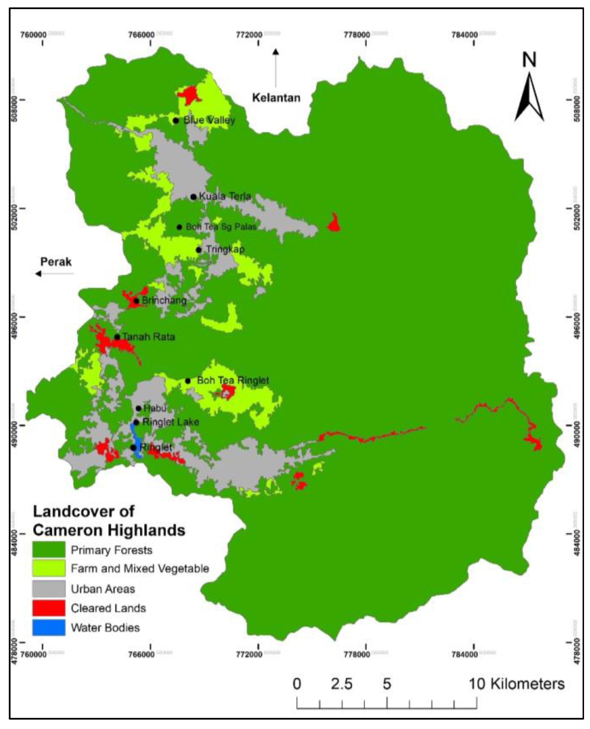
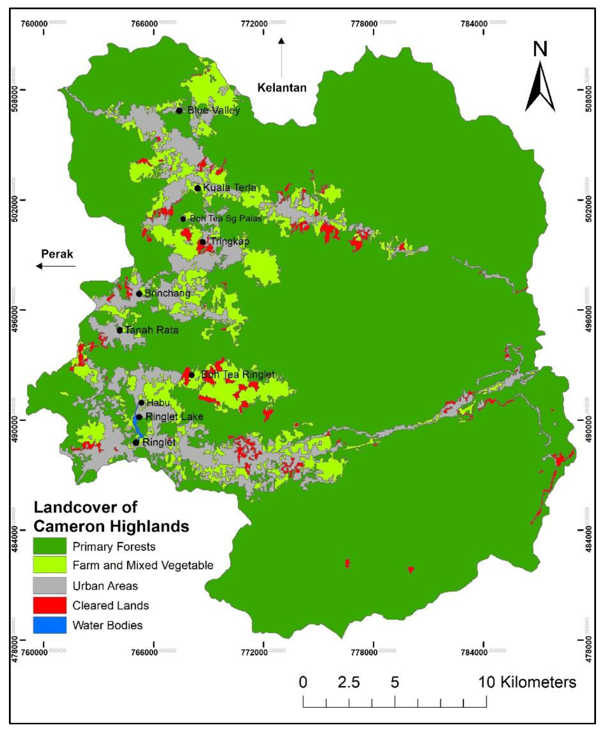
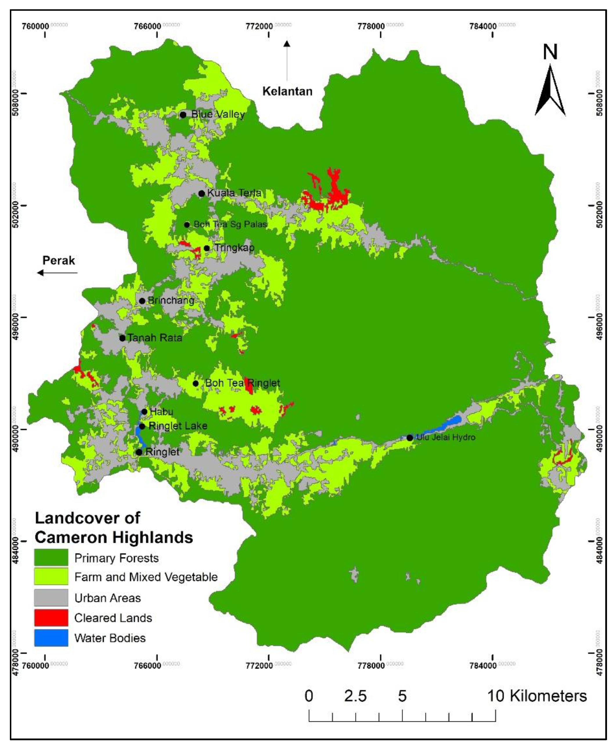
3.1. Land Cover Change Analysis

The highest class recorded for 2009 was primary forests (Figure 4) (578.15 km², 86.33% of total land area) followed by urban areas (50.10 km², 7.48%) and farm and mixed vegetables (33.00 km², 4.93%). The two minor land cover classes, namely cleared lands (7.84 km²) and water bodies (0.60 km²), were also recorded. The farm and mixed vegetables class includes tea plantations and other vegetation crops, such as corn, grapes, flowers, tomato, and strawberry farms. Within the farm and mixed vegetables land cover type, “other vegetation”, which comprises uses that are not individually categorized, account for only 1/10 of the total area. This is due to the lack of growth in area of these crop types in Cameron Highlands. Due to the limitations of Landsat 30 m resolution, these finer details are not able to be classified; hence, the difference can only be seen when higher resolution data are used.

In 2014, image classification results (Figure 5 and

Table 4. Land cover area change in Cameron Highlands.

	2009		2014		2019
	Area (sq. km)	Area (%)	Area (sq. km)	Area (%)	Area (sq. km)	Area (%)
Primary Forests	578.15	86.33%	541.76	80.90%	518.71	77.46%
Farm & Mixed Veg	33.00	4.93%	57.03	8.52%	84.61	12.63%
Urban Areas	50.10	7.48%	59.50	8.88%	61.10	9.12%
Cleared Lands	7.84	1.17%	11.06	1.65%	4.17	0.62%
Water Bodies	0.60	0.09%	0.34	0.05%	1.10	0.16%
Total	669.69	100.00%	669.69	100.00%	669.69	100.00%

) show that the highest class was also primary forest (541.76 km², accounting for 80.90% of the total land area and representing a decline of 36.39 km² compared to 2009), followed by urban areas (59.50 km², 8.88%), and farm and mixed vegetables (57.03 km², 8.52%). The remaining land cover classes were cleared lands (11.06 km²) and water bodies (0.34 km²). Large changes across the terrain and hilly areas of Cameron Highlands can be seen within a five-year period. Due to the continuous rise in both urban areas (9.40 km²) and farmland (24.03 km²), the decline of primary forests continues. Massive deforestation has occurred in the study area based on image interpretation and classification.

Illegal land clearing in small communities also contributes to the overall problem of deforestation. Although this may represent a small change, it is nonetheless an issue for the Land and Planning authorities of Cameron Highlands. This is because the areas of these activities are deep within the rainforest. Moreover, such uncontrolled activities might also be the result of landowners breaching the agreement of forest clearing, which is undertaken for plantations rather than the agreed purpose of urbanization. This may occur in other similar mountainous sites in addition to Cameron Highlands [49]. Predominantly in the areas of Kuala Terla, Tringkap, Brinchang, and Ringlet, in which numerous urban areas exist, it can be seen that farmlands are increasing in line with the decrease of urban housing. This could be due to the reduction in demand for housing areas and a rise in crop growth to meet the demand for western crops in the country. Towards the east, an area that was previously heavily forested has been cleared for land to build a road and a hydroelectric plant and is now categorized as an urban area. Land cover change during the study period is shown in Table 4.

Rapid forest degradation continues to expand until 2019. Figure 6 shows that the North East region of Cameron Highlands experienced land cover change due to construction of a road network, in addition to agriculture plots adjacent to the highway. Primary forest (518.71 km², accounting for 77.46% of total land area, a decline of 23.05 km² from 2014) was maintained as the highest class, followed by urban areas (61.10 km², 9.12%) and farm and mixed vegetables (84.61 km², 12.63%). The minor land cover classes of cleared lands and water bodies accounted for 1.10 and 4.17 km², respectively. A noticeable change, of −6.89 km², was found for the cleared land class, and a rise in water bodies of 0.76 km² (

Table 5. Difference in land cover growth between years.

Area between Years	09–14 (sq. km)	% Diff	14–19 (sq. km)	% Diff	09–19 (sq. km)	% Diff
Primary Forests	(−) 36.39	(−) 5.43%	(−) 23.05	(−) 3.44%	(−) 59.44	(−) 8.88%
Farm & Mixed Veg	(+) 24.03	(+) 3.59%	(+) 27.58	(+) 4.12%	(+) 51.61	(+) 7.71%
Urban Areas	(+) 9.40	(+) 1.40%	(+) 1.60	(+) 0.24%	(+) 11.00	(+) 1.64%
Cleared Lands	(+) 3.22	(+) 0.48%	(−) 6.89	(−) 1.03%	(−) 3.67	(−) 0.55%
Water Bodies	(−) 0.26	(−) 0.04%	(+) 0.76	(+) 0.11%	(+) 0.50	(+) 0.07%

). This change in water bodies is due to the operational status of the Ulu Jelai Hydroelectric dam. The trend of results obtained from this classification is consistent with the findings of Rendana et al. [26], Mohammadi et al. [50], and Razali et al. [51].

The accuracy of the OBIA classification for 2019 was validated using a ground-truthing assessment of GPS points collected from the study area. The results are applied in Figure 6. The producer’s accuracy value was 94.60% and the user’s accuracy value was 94.65%, resulting in an overall accuracy of 94.60%. Details of the confusion matrix table can be found in

Table 6. Confusion matrix table of 2019 land cover classification.

LULCC 2019	Cleared	Urban	Primary	Farm	Water	Total	User (%)
Cleared lands	95	1	0	0	0	96	98.96
Urban areas	3	92	1	7	0	103	89.32
Primary forests	0	2	97	4	0	103	94.17
Farm & Mixed vegetables	2	5	2	89	0	98	90.82
Water bodies	0	0	0	0	100	100	100.00
Total	100	100	100	100	100	500	94.65
Producers Accuracy (%)	95.00	92.00	97.00	89.00	100.00	94.60

. Notably, only the classification results of 2019 could be validated given the availability of GPS points, and images from other years were unable to be validated. Hence, for the years 2014 and 2009 (shown in

Table 7. Confusion matrix table of 2014 land cover classification.

LULCC 2014	Cleared	Urban	Primary	Farm	Water	Total	User (%)
Cleared lands	88	7	0	3	1	99	88.88
Urban areas	5	86	1	5	3	100	86.00
Primary forests	0	2	96	3	0	101	95.05
Farm & Mixed vegetables	8	1	3	88	0	100	88.00
Water bodies	0	3	0	0	97	100	97.00
Total	101	99	100	99	101	500	90.88
Producers Accuracy (%)	87.00	87.00	96.00	89.00	96.00	91.00

and

Table 8. Confusion matrix table of 2009 land cover classification.

LULCC 2009	Cleared	Urban	Primary	Farm	Water	Total	User (%)
Cleared lands	85	2	4	1	0	92	92.40
Urban areas	5	88	6	8	0	107	82.24
Primary forests	4	2	94	4	0	104	90.38
Farm & Mixed vegetables	2	5	2	89	0	98	90.82
Water bodies	0	1	0	0	98	99	98.99
Total	96	98	106	102	98	500	90.96
Producers Accuracy (%)	95.00	92.00	97.00	89.00	100.00	94.60

, respectively), the confusion matrix was derived using Google Earth to validate the accuracy (see Figure 7).

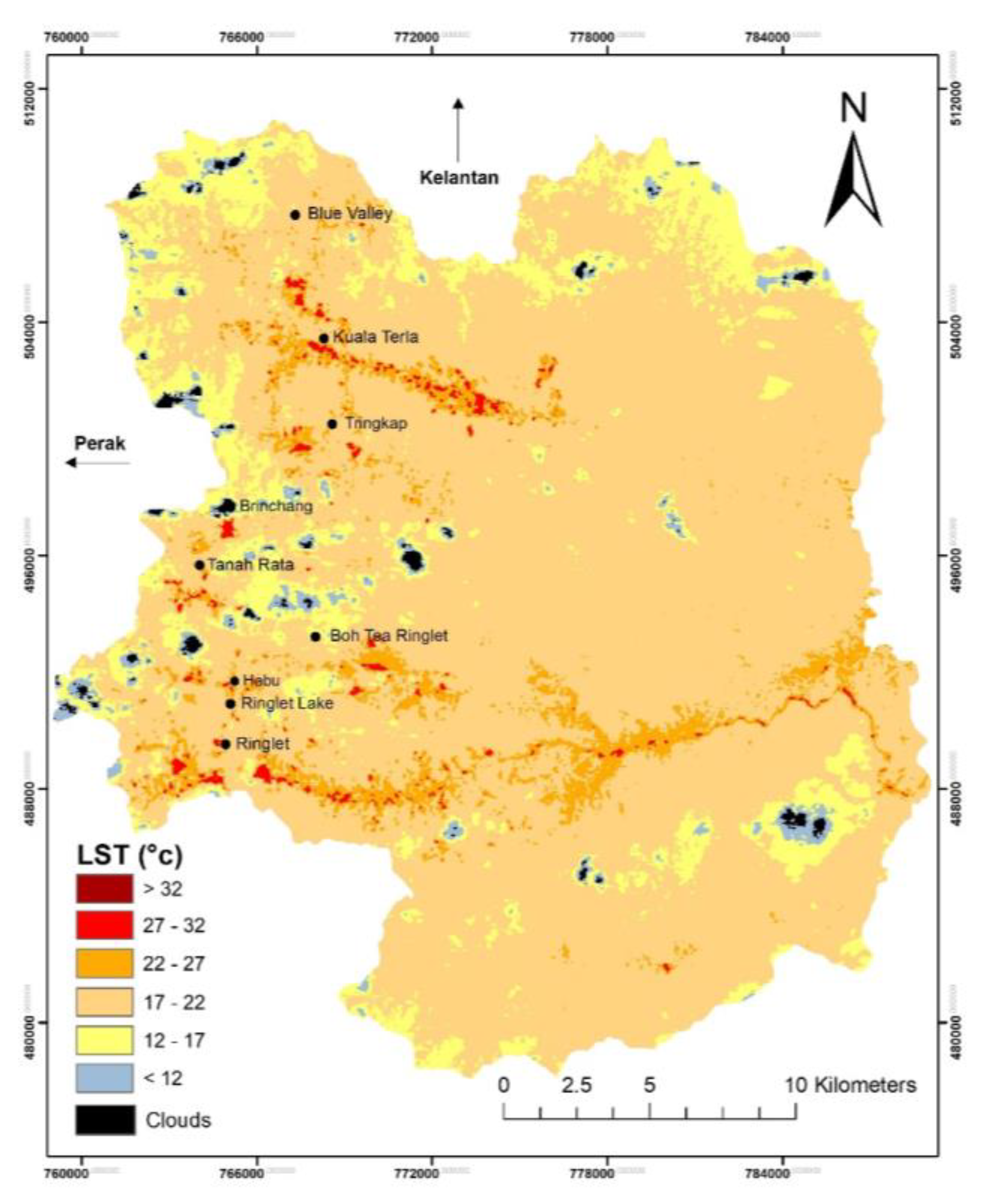
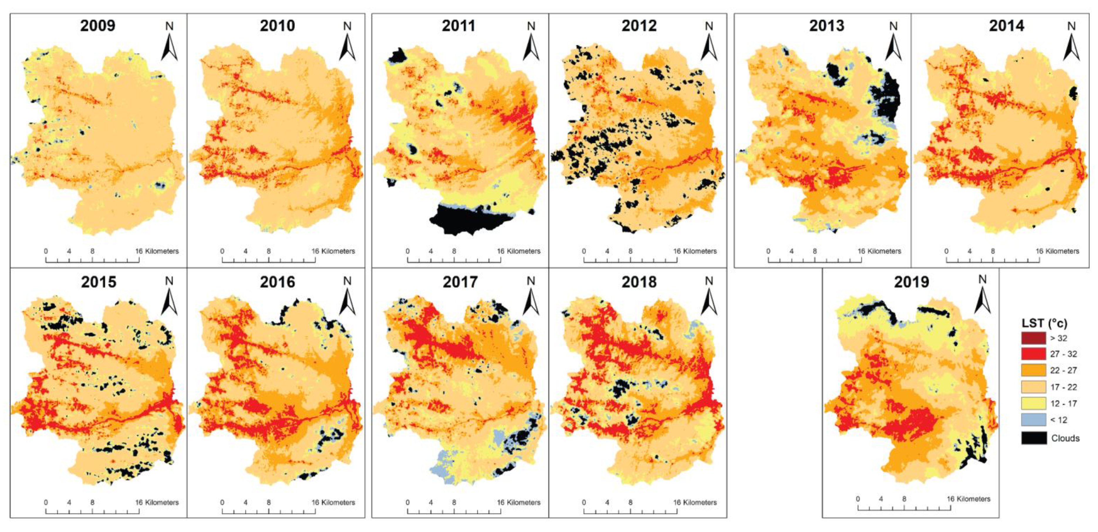
3.2. Land Surface Temperature Change Analysis Based on Landsat Satellite Data Compared to MODIS

High temperature values were concentrated in the populous towns of Brinchang, Ringlet, and Kuala Terla (Figure 8, for 2009;

Table 9. Temperature in °C of LST obtained from Landsat, Moderate Resolution Imaging Spectroradiometer (MODIS), and Met Malaysia.

		Temperature Platform (°C)
		Landsat (100 m)				MODIS (1 km)				Met Malaysia
Year	Month	Max	Min	Mean	SD	Max	Min	Mean	SD	Max	Min
2009	March	30.5	7.0	18.5	2.0	29.7	20.2	25.1	1.5	25.1	13.0
2010	February	34.4	15.7	21.3	1.6	28.5	21.0	24.3	1.4	24.8	13.0
2011	February	26.0	11.0	15.1	4.8	29.0	12.4	20.9	3.3	24.6	12.1
2012	April	36.6	9.0	19.8	3.5	28.2	12.2	24.6	1.6	24.4	14.2
2013	June	25.4	5.4	14.9	4.1	28.4	19.9	24.3	1.5	25.9	14.6
2014	March	40.9	13.8	23.4	1.9	31.1	22.0	25.6	1.5	25.5	11.8
2015	April	30.0	12.7	20.7	2.2	27.6	20.3	24.0	1.1	25.2	15.0
2016	April	34.7	12.1	23.9	2.1	32.0	22.0	26.7	1.8	26.4	15.1
2017	August	27.7	8.2	17.2	2.0	28.3	16.2	23.3	1.5	24.6	14.5
2018	January	33.7	9.4	20.5	2.0	31.0	14.1	24.3	2.2	24.5	13.9
2019	March	31.0	0.5	18.2	4.1	30.5	11.0	25.1	2.5	25.3	14.2

), with typical values ranging between 23 and 26 °C in the months of the first quarter. The results of LST retrieval from Landsat shows a similar range in temperature during April. The monsoon season peaks in the period from the end of January to the start of March, hence there was variability in temperatures during this period. High and low temperatures exhibited differences resulting from the cloud patterns and wind dynamics in the highland areas. As a result, it was difficult to obtain a consistent average for climate measures in the study area. Based on the results of Landsat alone (Figure 8 and Figure 9), it is difficult to ascertain the rise in temperatures relating to the deforestation pattern and the development of urban areas. Thus, the MODIS platform, in addition to air temperature data obtained from the Meteorological Department of Malaysia, was used as a guide to show the rising temperature trends.

The results are satisfactory with regards to a rising temperature, and this trend was observed after comparison with the multiple datasets. Although the rate of change is not as steep as previously thought, the change is clearly and steadily increasing. As shown in 2011, 2013, and 2019, due to cloud patterns and atmospheric conditions, it is difficult to comprehend the climate during this period; although other years show a better depiction of land surface temperature, this is a result of poor atmospheric correction effects [17,38,52]. By comparison, although MODIS shows lower variability of data between months, there are no absolute highs or lows, resulting in a more accurate depiction of the climate in Cameron Highlands. In 2014, the Landsat 8 sensor measured a maximum temperature of 40.9 °C, whereas MODIS recorded a maximum of 31.1 °C. A summary of the data can be seen in Table 9, which shows the relationship over time. Although the difference between the two sensors is significant, it is clear that the recorded temperature is correct due to the trend in rising temperatures.

3.3. Air Temperature against Landsat and MODIS.

Air temperature data were acquired from the Meteorological Department in Tanah Rata, Cameron Highlands. Maximum and minimum data for each month corresponding to the Landsat satellite data time frame are shown in Table 9. According to the data values from Met Malaysia, the highest recorded temperature was 26.4 °C, and the lowest temperature recorded was 11.8 °C. A negative difference denotes a higher estimation of LST compared to the recorded temperature, whereas a positive difference indicates a lower estimation compared to the recorded value. In the urban environment, the air temperature may vary in a broader range due to the urban heat index (UHI). For instance, the months of March and April display a higher temperature as the radiative energy emitted by the surface of pavements, vegetation, urban areas, soil, and water is at a maximum. This is due to an increase in the human influx to the region of Cameron Highlands, primarily due to an increase of visitors, and the passing of the monsoon season, which manifests as dry spells after the period of heavy rainfall [7,9]. The data are not relevant to the whole region but only to certain areas in which these data were taken from the weather retrieving nodes, because it is difficult to ascertain the “correct” temperature value for the region overall [53,54,55,56].

The year 2014 shows the highest deviation across all LST datasets with a minimum of −2 °C and maximum of −15.4 °C. The second highest deviation in temperature occurred in 2019, in which the minimum and maximum deviations were 13.7 and −5.7 °C, respectively. By comparison, a deviation between Met Malaysia and MODIS was found for 2014, with a minimum of −10.2 °C and a maximum of −5.6 °C (see

Table 10. Validation (difference) estimation against recorded LST in °C.

		Temperature Platform (°C)
		Landsat/MODIS		Met Malaysia/Landsat		Met Malaysia/MODIS
Year	Month	Max	Min	Max	Min	Max	Min
2009	March	0.8	−13.2	−5.4	6.0	−4.6	−7.2
2010	February	5.9	−5.3	−9.6	−2.7	−3.7	−8.0
2011	February	−3.0	−1.4	−1.4	1.1	−4.4	−0.3
2012	April	8.4	−3.2	−12.2	5.2	−3.8	2.0
2013	June	−3.0	−14.5	0.5	9.2	−2.5	−5.3
2014	March	9.8	−8.2	−15.4	−2.0	−5.6	−10.2
2015	April	2.4	−7.6	−4.8	2.3	−2.4	−5.3
2016	April	2.7	−9.9	−8.3	3.0	−5.6	−6.9
2017	August	−0.6	−8.0	−3.1	6.3	−3.7	−1.7
2018	January	−9.7	−8.4	3.2	8.2	−6.5	−0.2
2019	March	0.5	−10.5	−5.7	13.7	−5.2	3.2
Average Difference		1.3	−8.2	−5.6	4.6	−4.4	−3.6

). Clear skies are a major requirement for accurate LST retrieval. Thus, these unrealistic LST estimations are partly due to the erratic cloud coverage seen in 2011, 2013, 2018, and 2019 (Figure 9). Because the base image was not trained with a specific emissivity value in specific areas, the resulting image is as shown in the figure [12,17,18,33,35,38].

3.4. Verification of LST

To ensure the correctness of the results, the LST must be verified. For this purpose, we obtained data derived from MODIS imagery and air temperature data from the Meteorological Department of Malaysia with links to the station in Tanah Rata, Cameron Highlands. Initially, MODIS was reclassified to the same resolution as the Landsat TIRS sensor, that is 100 m; it is a challenge to ascertain the coverage of the LST using a pixel size of spatial resolution of 100 meters. Other challenges of this method of verification relate to uncertainty in the data quality, namely the correct calibration of the image and apparent implications for the data due to the sensor of the satellite. Air temperature data obtained at ground level was used to address these challenges [42].

Due to the vegetation cover of the study area, much of the vegetation canopy temperature was approximately equivalent to the surface air temperature [24]. Hence, the Landsat and MODIS data for this particular area (primary forest) can be considered a good reference for the air temperature recorded by the weather station.

Table 11. RMSE and bias of LST results.

LST Landsat–MODIS				LST MODIS–MetMY				LST Landsat–MetMY
Max		Min		Max		Min		Max		Min
RMSE	Bias	RMSE	Bias	RMSE	Bias	RMSE	Bias	RMSE	Bias	RMSE	Bias
4.68	2.41	8.76	−7.86	4.53	4.36	5.56	3.62	8.13	6.80	6.19	−4.20

shows various datasets which were subjected to a comparison of user predictions for the calculation of the required values. The LST values obtained from Landsat for 2009 to 2019 were averaged, and the associated Root Mean Square Error (RMSE) and bias values were derived. The reference LST was taken from MODIS for air temperature because this was considered to be accurate. It can be seen that the comparison of MODIS LST with local meteorological data has the lowest values relative to the other datasets. With an RMSE of 4.53 and 5.56 °C for maximum and minimum values, respectively, the results are reasonable and consistent, given the nature of the dataset at a spatial resolution of 100 m.

3.5. The LULC Effect on LST

Because the study area is covered mostly by vegetation, the area that is most stable in terms of LST changes across the map is primary forest. However, in many other areas, particularly towns, urban zones blend with secondary forests (parks, plantations, and areas of human-made vegetative recreation). These areas have a significant effect on the overall LST values because humans are carriers of heat and thus contribute to the anthropogenic heat distribution of a surrounding area. When this heat is massed, it tends to stick to nearby surfaces such as those of buildings. It is known that heat rises while cool air falls. Furthermore, the majority of buildings in the town areas of Cameron Highlands are living quarters with a minimum height of 10 stories and a maximum of 20 stories. The affected areas are Brinchang, Ringlet, and Tanah Rata, in which the population density is higher than that of other towns. These areas radiate an excess heat of 0.5 to 1.0 °C. Similarly, results from a study by Zhou et al. [22] showed that a similar urban environment in Austin, Texas, experienced a rise in temperature of 0.45 to 0.90 °C. The extent to which terrain factors affect the variation of LST depends on the intensity of external solar radiation on a given day. In his study, Zhao notes that the parks and forested regions of Austin have a cooling effect, in which the heat sinks of the area absorb heat and then release cold air.

In contrast, areas without parks display signs of overheating as a result of heat release, surface albedo, and an irregular complexity of landscape structures. Results obtained in the current study are similar to those of a study conducted in Oslo by Venter et al. [57] in which it was found that the temperature of the air was at least 0.6 °C higher in LST modelled using satellite imagery (in urban zones compared to the surrounding outer city). The authors used both Sentinel and Landsat as a means of comparison with meteorological data. The study clearly showed that the temperature of air increases through an impervious surface area paired with a decline of vegetation.

It has been found that the air temperature is at least 2–3 °C lower than the surface temperature depending on the altitude and surface type [48]. This is more evident in urban areas in which there are no pure vegetation pixels. Hence, the air temperature will be slightly lower (by 2–3 °C as previously mentioned) than the land surface temperature because ground radiation conduction is influenced by air particles [58,59]. In other regions of the world, studies have shown the usage of MODIS to estimate air temperature. In Northwest China, Lu et al. [60] conducted an experiment to determine the relationship between sensor temperature readings and on-site measurements. The results showed an RMSE between 2.39 and 3.05 °C; these results were dependent on seasonal and weather variability. Additionally, in the North Tibetan plateau of China, Zhu et al. [61] compared MODIS with air temperature to derive an RMSE of 7.45 °C and a bias of 6.21 °C. The cause of these higher values was attributed to the presence of cloud pixels and haze surrounding the study area. In Egypt, El Kenawy et al. [53] reported an average estimation of 5 °C according to seasonal change. These results are consistent with those of the present study, in which we derived RMSE values ranging between 4.53 and 8.13 °C for different sensor comparisons. Furthermore, Gomis-Cebolla et al. [62] studied the use of LST from MODIS to compare with locally extracted air temperature values in the Amazon rainforest. The study reported RMSE values between 1.58 and 1.85 °C. Because the study was carried out during the winter, the expected RMSE was below estimation. By comparison, if the study was conducted during the summer, the RMSE would be expected to be between 4 and 5 °C.

Various studies of Asian cities comparable in size and density have observed an excess of anthropogenic heating as high as 1.5 °C [21,48,63,64,65]. A study by Wang et al. [66] conducted in Kuala Lumpur states that “air temperature is a good comparison against satellite-based data obtained temperatures, however, they do not reflect on the ‘true’ temperate climate of a surrounding area with a multitude of external implications such as wind speed, time, body induced heat radiation as well as heat created from vehicles”. This statement is also supported by the study of Kong et al. [45], in which air temperature data also showed signs of outliers, mostly consisting of highs during the summer months of April to June, with estimated values of 0.3–0.5 °C. This could be a case of radiative heat being trapped amongst buildings or another case of climate-induced change as a result of increased influx into the region.

Cameron Highlands is known as a mountainous region with a climatology different from that of surrounding areas. Hence, multiple changes in temperature are frequent throughout the day. When paired with sudden changes in wind speed (which range on average from 2 to 3.4 kmph), this variation leads to uncertainty in the daily average temperature values. It should be noted that the undulating terrain of Cameron Highlands makes it difficult for heat to be radiated smoothly compared to the flatlands. This is more evident when various tall structures hinder the flow of air. Analysis of LST conducted in primary forests in urban areas reveal a higher pattern than LST of primary forests in a mixed zone of urban land cover. Portions of secondary forests are covered with glass roofing, whereas others have aluminum roofing. Furthermore, these roofs are either black in color or comprised of gray cloth to keep insects out. We classified these areas as secondary forests despite their signature showing as an urban zone due to surface reflectance. Notably, these areas have a similar pattern in their retention of heat to that of urban areas because plantations are situated below aluminum roofs [67]. Thus, heat will further radiate in these areas, thus contributing to an increase in the value of the overall LST, because these manmade objects do not regulate LST in the same way as natural objects [68,69]. A more significant surface area density of buildings has a proportionate relationship to high urbanization and, in turn, a weaker LST regulation ability. This results in an increase in the massing of local heat, in addition to increases in the urban heat Index (UHI) and LST. Therefore, it is vital to take note of these particular areas that might affect the overall distribution of LST.

4. Conclusions

This study explores the LULC and LST for the years 2009 and 2019 based on Landsat and MODIS data. Due to constant population growth in an environment of already cramped spaces for the expansion of urban housing, future trends for our tropical rainforests appear to be inevitable. Results obtained from this study show that the total urban area increased by almost 1.70% since 2009, and farmland and agriculture plots registered a significant 7.71% increase. Combined, these changes led to a decrease in primary forest cover of 8.88%. Particular areas of concern in the already crowded urban region are Tanah Rata and Brinchang due to the ongoing change in LULC. Due to the nature of the terrain and the historical record of landslides occurring in the area, it can be concluded that the area is highly susceptible to natural disasters. Irreversible actions and consequences may eventuate if further development and deforestation occur in the area. Changes in land use and land cover (LULC) over time have also affected the distribution of land cover areas, namely conversion of land cover types from either already deforested primary forests to urban areas, or towards further agriculture usage. Accuracy proved successful using on-site collected GPS points (94.60%). Further analysis is recommended with the use of high-resolution image sensors; Sentinel (10 m) and PlanetScope (3 m) could be considered. Using these image sensors, finer details can be extracted for an LULC classification, which would yield more classes and provide a more accurate description of the study site.

The land surface temperature showed a rapidly increasing trend, particularly in the urban areas of Cameron Highlands, in particular, Kuala Terla and Ringlet. During a ten-year period, the recorded temperatures showed a rise of about 2–3 °C across all channels, with an extreme of 5 °C on average. The use of Landsat 8 with the SWA method proved reasonable with the results obtained, although outliers arose partly due to the pre-processing stage. However, MODIS and weather data from Met Malaysia confirmed a rise in the region of LST, the primary focus of this study. It is recommended that the calibration of LST data be undertaken in future projects to avoid the uncertainty of erratic LST values as a result of cloud coverage. The results of this study suggest that LST is heavily dependent on seasonal radiation conditions mainly due to the monsoon season and its subsequent effects, which cause the overestimation of cooling values. Due to the undulating terrain of Cameron Highlands, which has a gradient of multiple forest altitude classes, future studies should calculate LST at different forest altitudes and take into account the forest cooling effect and the urban heat index. Population density also plays a role in the acquired LST values, in which concentrated portions of the study area displayed higher temperature values compared to smaller towns. Furthermore, thermal infrared remote sensing applications could be adapted for future studies to allow for better measurement of heat radiation in concentrated urban areas. Ground-based temperature data in towns can provide more accurate insights into urban heat indexes and their effect on air temperature. Correct usage of water vapor data for each zone should be taken into account in future studies, in addition to considering the use of Advanced Spaceborne Thermal Emission and Reflection Radiometer (ASTER) and Advanced Very-High-Resolution Radiometer (AVHRR) data. Research results provide a fuller understanding of the drivers of increased LST, which is mainly due to increased demand for urbanization and, in turn, is linked to the expansion of deforestation. However, it is a challenge to prevent urbanization without a change in the decision making of upper management. Thus, it is suggested that the state government authority considers enacting policies and strategies that support the control of deforestation in the highlands. This will address ecological and environmental concerns and help ensure that development takes place sustainably.

References

1. Kumaran, S.; Ainuddin, A.N. Forest, water and climate of Cameron Highlands. In Proceedings of the Seminar on Sustainable Development of Cameron Highlands, Brinchang, Cameron Highlands, Malaysia, 11–12 December 2004; p. 11. [Google Scholar]
2. Jin, M. Analysis of land skin temperature using AVHRR observations. Bull. Am. Meteorol. Soc. 2004, 85, 587–600. [Google Scholar] [CrossRef]
3. Hardwick, S.; Toumi, R.; Pfeifer, M.; Turner, E.; Nilus, R.; Ewers, R. The relationship between leaf area index and microclimate in tropical forest and oil palm plantation: Forest disturbance drives changes in microclimate. Agric. For. Meteorol. 2015, 201, 187–195. [Google Scholar] [CrossRef] [PubMed] [Green Version]
4. Knight, J.; Harrison, S. The impacts of climate change on terrestrial Earth surface systems. Nat. Clim. Chang. 2012, 3, 24–29. [Google Scholar] [CrossRef]
5. Beniston, M. Mountain Environments in Changing Climates; Routledge Publishing Company: Abingdon, UK, 1994; p. 492. [Google Scholar]
6. Wolff, N.; Masuda, Y.; Meijaard, E.; Wells, J.; Game, E. Impacts of tropical deforestation on local temperature and human well-being perceptions. Glob. Environ. Chang. 2018, 52, 181–189. [Google Scholar] [CrossRef]
7. Cong, R.; Brady, M. The interdependence between rainfall and temperature: Copula analyses. Sci. World J. 2012, 1–11. [Google Scholar] [CrossRef] [PubMed] [Green Version]
8. World Meteorological Organisation. Climate and Land Degradation. Soil conservation—Land Management—Flood Forecasting—Food Security. WMO—No 989. Available online: http://www.wamis.org/agm/pubs/brochures/wmo989e.pdf (accessed on 17 December 2019).
9. Berg, P.; Moseley, C.; Haerter, J. Strong increase in convective precipitation in response to higher temperatures. Nat. Geosci. 2013, 6, 181–185. [Google Scholar] [CrossRef]
10. Avdan, U.; Jovanovska, G. Algorithm for automated mapping of land surface temperature using LANDSAT 8 satellite data. J. Sens. 2016, 1–8. [Google Scholar] [CrossRef] [Green Version]
11. Darge, Y.; Hailu, B.; Muluneh, A.; Kidane, T. Detection of geothermal anomalies using Landsat 8 TIRS data in Tulu Moye geothermal prospect, main ethiopian rift. Int. J. Appl. Earth Obs. Geoinf. 2019, 74, 16–26. [Google Scholar] [CrossRef]
12. Sahana, M.; Ahmed, R.; Sajjad, H. Analysing land surface temperature distribution in response to land use/land cover change using split window algorithm and spectral radiance model in Sundarban Biosphere Reserve, India. Modeling Earth Syst. Environ. 2016, 2. [Google Scholar] [CrossRef] [Green Version]
13. Cristóbal, J.; Jiménez-Muñoz, J.; Prakash, A.; Mattar, C.; Skoković, D.; Sobrino, J. An improved single-channel method to retrieve land surface temperature from the Landsat-8 thermal band. Remote Sens. 2018, 10, 431. [Google Scholar] [CrossRef] [Green Version]
14. Montanaro, M.; Lunsford, A.; Tesfaye, Z.; Wenny, B.; Reuter, D. Radiometric calibration methodology of the Landsat 8 thermal infrared sensor. Remote Sens. 2014, 6, 8803–8821. [Google Scholar] [CrossRef] [Green Version]
15. USGS1. Using the USGS Landsat 8 Product. 2018. Available online: https://www.usgs.gov/media/files/landsat-8-data-users-handbook (accessed on 25 April 2019).
16. USGS2. Landsat 8 (L8) Operational Land Imager (OLI) and Thermal Infrared Sensor (TIRS). 2018. Available online: http://landsat.usgs.gov/calibration_notices.php (accessed on 25 April 2019).
17. Al Kafy, A.; Al-Faisal, A.; Mahmudul Hasan, M.; Sikdar, M.; Hasan Khan, M.; Rahman, M.; Islam, R. Impact of LULC changes on LST in Rajshahi district of Bangladesh: A remote sensing approach. J. Geogr. Studies 2020, 3, 11–23. [Google Scholar] [CrossRef]
18. Ogunode, A.; Akombelwa, M. An algorithm to retrieve land surface temperature using Landsat-8 dataset. South Afr. J. Geomat. 2017, 6, 262. [Google Scholar] [CrossRef]
19. Rozenstein, O.; Qin, Z.; Derimian, Y.; Karnieli, A. Derivation of land surface temperature for Landsat-8 tirs using a split window algorithm. Sensors 2014, 14, 5768–5780. [Google Scholar] [CrossRef] [PubMed]
20. Sajib, M.; Wang, T. Estimation of Land Surface Temperature in an agricultural region of Bangladesh from Landsat 8: Intercomparison of four algorithms. Sensors 2020, 20, 1778. [Google Scholar] [CrossRef] [Green Version]
21. Wang, L.; Lu, Y.; Yao, Y. Comparison of three algorithms for the retrieval of land surface temperature from Landsat 8 images. Sensors 2019, 19, 5049. [Google Scholar] [CrossRef] [Green Version]
22. Zhou, D.; Xiao, J.; Bonafoni, S.; Berger, C.; Deilami, K.; Zhou, Y.; Frolkin, S.; Yao, R.; Qiao, Z.; Sobrino, J.A. Satellite remote sensing of surface urban heat islands: Progress, challenges, and perspectives. Remote Sens. 2018, 11, 48. [Google Scholar] [CrossRef] [Green Version]
23. Mejbel Salih, M.; Zakariya Jasim, O.; Hassoon, K.I.; Jameel Abdalkadhum, A. Land surface temperature retrieval from LANDSAT-8 thermal infrared sensor data and validation with infrared thermometer camera. Int. J. Eng. Technol. 2018, 7, 608. [Google Scholar] [CrossRef] [Green Version]
24. Nemani, R.; Running, S. Estimation of regional surface resistance to evapotranspiration from NDVI and Thermal-IR AVHRR data. J. Appl. Meteorol. 1989, 28, 276–284. [Google Scholar] [CrossRef]
25. Akmar, C.K.; Mohd Hasmadi, I. Land use in cameron highlands: Analysis of its changes from space. In Proceedings of the World Engineering Congress: Geometrics and Geographical Information Science, Grand Margherita Hotel, Kuching, Sarawak, Malaysia, 2–5 August 2010; pp. 190–195. [Google Scholar]
26. Rendana, M.; Rahim, S.; Idris, W.; Lihan, T.; Rahman, Z. CA-Markov for predicting land use changes in tropical catchment area: A case study in cameron Highland, Malaysia. J. Appl. Sci. 2015, 15, 689–695. [Google Scholar] [CrossRef] [Green Version]
27. Jabatan Meteorologi Malaysia. 2019. Cameron Highlands Temperature 2009–2019. Available online: https://www.met.gov.my/ (accessed on 30 September 2019).
28. Yin, G.; Mariethoz, G.; McCabe, M. Gap-filling of Landsat 7 imagery using the direct sampling method. Remote Sens. 2016, 9, 12. [Google Scholar] [CrossRef] [Green Version]
29. Wang, X.; Liu, S.; Du, P.; Liang, H.; Xia, J.; Li, Y. Object-based change detection in urban areas from high spatial resolution images based on multiple features and ensemble learning. Remote Sens. 2018, 10, 276. [Google Scholar] [CrossRef] [Green Version]
30. Yusoff, N.; Muharam, F. The use of multi-temporal landsat imageries in detecting seasonal crop abandonment. Remote Sens. 2015, 7, 11974–11991. [Google Scholar] [CrossRef] [Green Version]
31. Le Bas, T. RSOBIA—A new OBIA Toolbar and Toolbox in ArcMap 10.x for Segmentation and Classification. GEOBIA 2016. [Google Scholar] [CrossRef]
32. Tavares, M.H.; Cunha, A.H.F.; Motta-Marques, D.; Ruhoff, A.L.; Cavalcanti, J.R.; Fragoso, C.R., Jr.; Bravo, J.M.; Munar, A.M.; Fan, F.M.; Rodrigues, L.H.R. Comparison of methods to estimate lake-surface-water temperature using Landsat 7 ETM+ and MODIS imagery: Case study of a large shallow subtropical lake in southern Brazil. Water 2019, 11, 168. [Google Scholar] [CrossRef] [Green Version]
33. Nguemhe Fils, S.; Mimba, M.; Dzana, J.; Etouna, J.; Mounoumeck, P.; Hakdaoui, M. TM/ETM+/LDCM images for studying land surface temperature (LST) interplay with impervious surfaces changes over time within the douala Metropolis, Cameroon. J. Indian Soc. Remote Sens. 2017, 46, 131–143. [Google Scholar] [CrossRef]
34. Hesslerová, P.; Huryna, H.; Pokorný, J.; Procházka, J. The effect of forest disturbance on landscape temperature. Ecol. Eng. 2018, 120, 345–354. [Google Scholar] [CrossRef]
35. Kumari, B.; Tayyab, M.; Shahfahad, S.; Mallick, J.; Khan, M.; Rahman, A. Satellite-driven land surface temperature (LST) using Landsat 5, 7 (TM/ETM+ SLC) and Landsat 8 (OLI/TIRS) data and its association with built-up and green cover over urban Delhi, India. Remote Sens. Earth Syst. Sci. 2018, 1, 63–78. [Google Scholar] [CrossRef]
36. Walawender, J.; Szymanowski, M.; Hajto, M.; Bokwa, A. Land surface temperature patterns in the urban agglomeration of Krakow (Poland) derived from Landsat-7/ETM+ data. Pure Appl. Geophys. 2013, 171, 913–940. [Google Scholar] [CrossRef] [Green Version]
37. Atitar, M.; Sobrino, J. A split-window algorithm for estimating LST from meteosat 9 data: Test and comparison with data and MODIS LSTs. IEEE Geosci. Remote Sens. Lett. 2009, 6, 122–126. [Google Scholar] [CrossRef]
38. Jiménez-Muñoz, J.; Sobrino, J. Error sources on the land surface temperature retrieved from thermal infrared single channel remote sensing data. Int. J. Remote Sens. 2006, 27, 999–1014. [Google Scholar] [CrossRef]
39. Yu, X.; Guo, X.; Wu, Z. Land surface temperature retrieval from Landsat 8 TIRS—Comparison between radiative transfer equation-based method, split window algorithm and single channel method. Remote Sens. 2014, 6, 9829–9852. [Google Scholar] [CrossRef] [Green Version]
40. USGS. Landsat 7 ETM+ Calibration Notices. 2017. Available online: https://www.usgs.gov/land-resources/nli/landsat/landsat-7-etm-calibration-notices (accessed on 21 April 2019).
41. Jarraud, M. Guide to Meteorological Instruments and Methods of Observation (wmo-no. 8); World meteorological organisation: Geneva, Switzerland, 2008. [Google Scholar]
42. Mcrae, G.J. A simple procedure for calculating atmospheric water vapor concentration. J. Air Pollut. Control Assoc. 1980, 30, 394. [Google Scholar] [CrossRef]
43. Dutta, R. Remote sensing of energy fluxes and soil moisture content. J. Spat. Sci. 2015, 60, 196–197. [Google Scholar] [CrossRef]
44. Jimenez-Munoz, J.; Sobrino, J.; Skokovic, D.; Mattar, C.; Cristobal, J. Land surface temperature retrieval methods from Landsat-8 thermal infrared sensor data. IEEE Geosci. Remote Sens. Lett. 2014, 11, 1840–1843. [Google Scholar] [CrossRef]
45. Kong, F.; Yin, H.; James, P.; Hutyra, L.; He, H. Effects of spatial pattern of greenspace on urban cooling in a large metropolitan area of eastern China. Landsc. Urban Plan. 2014, 128, 35–47. [Google Scholar] [CrossRef]
46. Isaya Ndossi, M.; Avdan, U. Application of Open Source Coding Technologies in the Production of Land Surface Temperature (LST) Maps from Landsat: A PyQGIS Plugin. Remote Sens. 2016, 8, 413. [Google Scholar] [CrossRef] [Green Version]
47. Jimenez-Munoz, J.; Sobrino, J. Split-window coefficients for land surface temperature retrieval from low-resolution thermal infrared sensors. IEEE Geosci. Remote Sens. Lett. 2008, 5, 806–809. [Google Scholar] [CrossRef]
48. Li, Z.; Gu, X.; Dixon, P.; He, Y. Applicability of Land Surface Temperature (LST) estimates from AVHRR satellite image composites in northern Canada 2019. Available online: http://hdl.handle.net/1807/69334 (accessed on 15 March 2020).
49. Islam, K.; Jashimuddin, M.; Nath, B.; Nath, T. Land use classification and change detection by using multi-temporal remotely sensed imagery: The case of Chunati wildlife sanctuary, Bangladesh. Egypt. J. Remote Sens. Space Sci. 2018, 21, 37–47. [Google Scholar] [CrossRef]
50. Mohammadi, A.; Baharin, B.; Shahabi, H. Land cover mapping using a novel combination model of satellite imageries: Case study of a part of the Cameron Highlands, Pahang, Malaysia. Appl. Ecol. Environ. Res. 2018, 17, 1835–1848. [Google Scholar] [CrossRef]
51. Razali, A.; Syed Ismail, S.; Awang, S.; Praveena, S.; Zainal Abidin, E. Land use change in highland area and its impact on river water quality: A review of case studies in Malaysia. Ecol. Process. 2018, 7. [Google Scholar] [CrossRef] [Green Version]
52. Chen, X.; Zhao, H.; Li, P.; Yin, Z. Remote sensing image-based analysis of the relationship between urban heat island and land use/cover changes. Remote Sens. Environ. 2006, 104, 133–146. [Google Scholar] [CrossRef]
53. El Kenawy, A.M.; Hereher, M.E.; Robaa, S.M. An assessment of the accuracy of MODIS land surface temperature over Egypt using ground-based measurements. Remote Sens. 2019, 11, 2369. [Google Scholar] [CrossRef] [Green Version]
54. Gallo, K.; Hale, R.; Tarpley, D.; Yu, Y. Evaluation of the relationship between air and land surface temperature under clear and cloudy-sky conditions. J. Appl. Meteorol. Climatol. 2011, 50, 767–775. [Google Scholar] [CrossRef]
55. Kaplan, G.; Avdan, U.; Avdan, Z. Urban heat island analysis using the Landsat 8 satellite data: A case study in Skopje, Macedonia. Proceedings 2018, 2, 358. [Google Scholar] [CrossRef] [Green Version]
56. Liu, S.; Su, H.; Zhang, R.; Tian, J.; Wang, W. Estimating the surface air temperature by remote sensing in northwest China using an improved advection-energy balance for air temperature model. Adv. Meteorol. 2016, 1–11. [Google Scholar] [CrossRef] [Green Version]
57. Venter, Z.; Brousse, O.; Esau, I.; Meier, F. Hyperlocal mapping of urban air temperature using remote sensing and crowdsourced weather data. Remote Sens. Environ. 2020, 242, 111791. [Google Scholar] [CrossRef]
58. Prihodko, L.; Goward, S. Estimation of air temperature from remotely sensed surface observations. Remote Sens. Environ. 1997, 60, 335–346. [Google Scholar] [CrossRef]
59. Zeng, L.; Wardlow, B.; Tadesse, T.; Shan, J.; Hayes, M.; Li, D.; Xiang, D. Estimation of daily air temperature based on MODIS land surface temperature products over the corn belt in the US. Remote Sens. 2015, 7, 951–970. [Google Scholar] [CrossRef] [Green Version]
60. Lu, L.; Zhang, T.; Wang, T.; Zhou, X. Evaluation of collection-6 MODIS land surface temperature product using multi-year ground measurements in an arid area of northwest China. Remote Sens. 2018, 10, 1852. [Google Scholar] [CrossRef] [Green Version]
61. Zhu, W.; Lu, A.; Jia, S. Estimation of daily maximum and minimum air temperature using MODIS land surface temperature products. Remote Sens. Environ. 2013, 130, 62–73. [Google Scholar] [CrossRef]
62. Gomis-Cebolla, J.; Jimenez, J.; Sobrino, J. LST retrieval algorithm adapted to the Amazon evergreen forests using MODIS data. Remote Sens. Environ. 2018, 204, 401–411. [Google Scholar] [CrossRef]
63. Ichinose, T.; Shimodozono, K.; Hanaki, K. Impact of anthropogenic heat on urban climate in Tokyo. Atmos Environ. 1999, 33, 3897–3909. [Google Scholar] [CrossRef]
64. Jin, M.; Li, J.; Wang, C.; Shang, R. A Practical split-window algorithm for retrieving land surface temperature from Landsat-8 data and a case study of an urban area in China. Remote Sens. 2015, 7, 4371–4390. [Google Scholar] [CrossRef] [Green Version]
65. Wang, Y.; Li, Y.; Sabatino, S.; Martilli, A.; Chan, P. Effects of anthropogenic heat due to air-conditioning systems on an extreme high temperature event in Hong Kong. Environ. Res. Lett. 2018, 1, 034015. [Google Scholar] [CrossRef]
66. Wang, K.; Aktas, Y.; Stocker, J.; Carruthers, D.; Hunt, J.; Malki-Epshtein, L. Urban heat island modelling of a tropical city: Case of Kuala Lumpur. Geosci. Lett. 2019, 6. [Google Scholar] [CrossRef]
67. Ejiagha, I.; Ahmed, M.; Hassan, Q.; Dewan, A.; Gupta, A.; Rangelova, E. Use of remote sensing in comprehending the influence of urban landscape’s composition and configuration on land surface temperature at neighbourhood scale. Remote Sens. 2020, 12, 2508. [Google Scholar] [CrossRef]
68. Cao, X.; Onishi, A.; Chen, J.; Imura, H. Quantifying the cool island intensity of urban parks using ASTER and IKONOS data. Landsc. Urban Plan. 2010, 96, 224–231. [Google Scholar] [CrossRef]
69. Du, H.; Song, X.; Jiang, H.; Kan, Z.; Wang, Z.; Cai, Y. Research on the cooling island effects of water body: A case study of Shanghai, China. Ecol. Indic. 2016, 67, 31–38. [Google Scholar] [CrossRef]
Figure 1. Study site of Cameron Highlands district (in the dark green shaded area), in the state of Pahang (light green), bordering Perak to the west and Kelantan to the north.
Land 09 00372 g001
Figure 2. Band combination 5,4,3 shown in image (A) (Ringlet lake in the middle surrounded by primary forests in dense red, while urban areas are shown as light gray), (B) (primary forest surrounds urban areas and farms. Farms can be distinguished by the slightly reddish tone with a mixture of light green) and (C) (cleared lands seen with a bare earth color, white-gray amidst primary forest around). Band combination 6,5,4 shown in image (D) (cleared lands has a light brown color in a lighter green tone of farms. Cleared lands are also identified as a lighter brown-white color tone when it has been cleared for weeks and left under the sun), (E) (urban areas in a purple tone surrounded by farms seen as light pink), (F) (water bodies-Ulu Jelai hydroelectric plant. Urban area towards the east of the dam in a light brown-purple color tone. The area is surrounded by primary forests seen as a darker shade of green; similarly, in (D)).
Land 09 00372 g002
Figure 3. Image analysis retrieval flowchart.
Land 09 00372 g003
Figure 4. Land cover classification of Cameron Highlands in 2009.
Land 09 00372 g004
Figure 5. Land cover classification of Cameron Highlands in 2014.
Land 09 00372 g005
Figure 6. Land cover classification of Cameron Highlands in 2019.
Land 09 00372 g006
Figure 7. Test accuracy using Google Maps for years 2009 and 2014. GPS points used for year 2019.
Land 09 00372 g007
Figure 8. Land surface temperature (LST) for 2009 in Cameron Highlands with place markers to denote areas of interest.
Land 09 00372 g008
Figure 9. Images showing land surface temperature for the period 2009–2019.
Land 09 00372 g009