Quantifying Climate-Wise Connectivity across a Topographically Diverse Landscape


1
Department of Environmental Science, Policy, and Management, University of California at Berkeley, Berkeley, CA 94720, USA
2
Dwight Center for Conservation Science, Pepperwood, Santa Rosa, CA 95404, USA
*
Author to whom correspondence should be addressed.
Land 2020, 9(10), 355; https://doi.org/10.3390/land9100355
Submission received: 15 August 2020
/
Revised: 19 September 2020
/
Accepted: 24 September 2020
/
Published: 26 September 2020
(This article belongs to the Special Issue Dynamic Landscape Connectivity)
Abstract
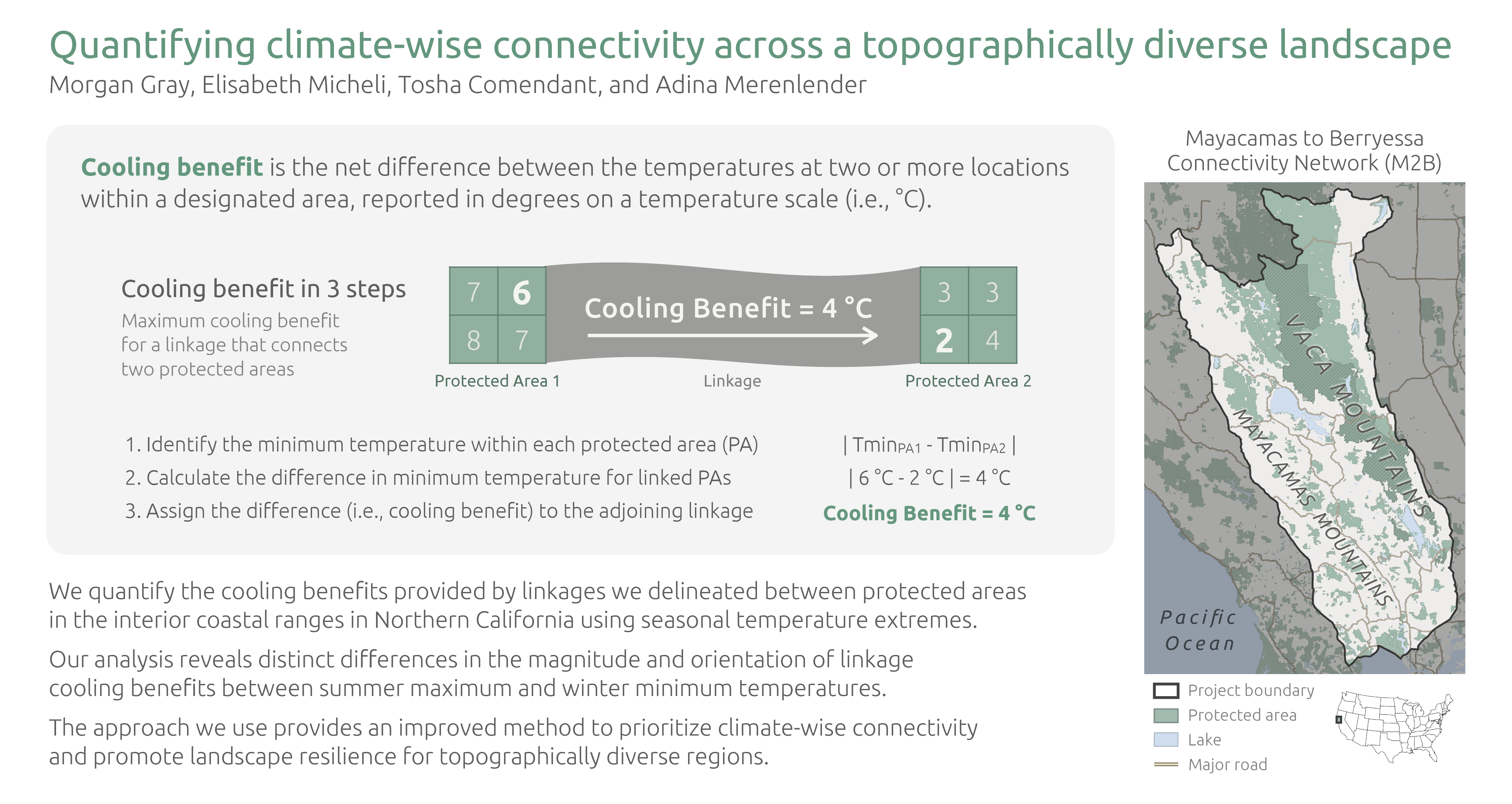
:Climate-wise connectivity is essential to provide species access to suitable habitats in the future, yet we lack a consistent means of quantifying climate adaptation benefits of habitat linkages. Species range shifts to cooler climates have been widely observed, suggesting we should protect pathways providing access to cooler locations. However, in topographically diverse regions, the effects of elevation, seasonality, and proximity to large water bodies are complex drivers of biologically relevant temperature gradients. Here, we identify potential terrestrial and riparian linkages and their cooling benefit using mid-century summer and winter temperature extremes for interior coastal ranges in Northern California. It is rare for the same area to possess both terrestrial and riparian connectivity value. Our analysis reveals distinct differences in the magnitude and orientation of cooling benefits between the summer maximum and winter minimum temperatures provided by the linkages we delineated for the area. The cooling benefits for both linkage types were maximized to the west during summer, but upslope and to the northeast during winter. The approach we employ here provides an improved method to prioritize climate-wise connectivity and promote landscape resilience for topographically diverse regions.

1. Introduction
Anthropogenic climate change is impelling a redistribution of species, with pervasive and substantial impacts on ecosystem function and human well-being, on every continent [1]. As the climate warms, species must tolerate the change, move, adapt, or face local and possibly global extinction [2]. Changes in climatic conditions will, in many cases, pressure plants and animals to shift from current to more suitable areas in the future [3,4]. Such range shifts toward cooler locations have been documented for a wide variety of species [5,6,7,8,9]. Species that cannot track shifting climate conditions by changing their location as needed are at risk of detrimental genetic effects, increased disease susceptibility, and greater risk of extinction [10,11,12,13].
Connectivity to facilitate range shifts will likely be necessary for many species to adapt to the changing climate [14]. Connectivity is a measure of how well a landscape promotes the movement of organisms and resources [15] and is one of the most commonly cited conservation strategies for climate adaptation [16]. We define linkage as a broad swath of land that provides potential connectivity between larger habitat areas, and reserve the word corridor for a collection of parcels designated for conservation action. Land conversion, natural habitat loss, fragmentation, and other human activities that decrease connectivity are increasing worldwide [17]. For example, estimates of human modification, such as land-use and the density of linear infrastructure (e.g., roads and fences), in particular, have been shown to be barriers to movement for five wide-ranging species [18]. The need to counteract this type of fragmentation has been recognized for many decades, and conservation efforts focused on enhancing connectivity are wide ranging as a way to promote population and ecosystem resilience [16,19].
Changes in climatic conditions will, in many cases, shift the location and availability of suitable habitat, necessitating directional movements from current to future areas of climatic and habitat suitability [3]. Therefore, climate-wise connectivity methods have emerged recently and emphasize establishing corridors between existing habitat patches and those that will be suitable in the future to facilitate species range shifts [20]. Selecting the best methods for site-specific climate-wise connectivity design depends on the conservation objectives, available data, and landscape attributes. A commonly used strategy is to generate models that predict the future range for one or more species, and then delineate linkages based on potential routes between projected and currently suitable locations, e.g., [21,22,23]. However, the utility of these approaches is limited by the need for dispersal and other life history data from a truly representative number of species and the high levels of uncertainty inherent in species distribution models.
An alternative approach is to forego an explicit reliance on species characteristics and movement patterns, instead prioritizing connections based on structural landscape features expected to provide species with the time and habitat needed to track a changing climate. This concept has been applied to identify a range of potential connections, including linkages that track climate gradients [24,25]; minimize the rate at which species would have to move to maintain constant climate conditions [26]; provide indicators of climate stability [27,28,29]; and connect current and future climate analogs [4,30].
Structural connectivity methods rely on existing environmental and climatic gradients or enduring geophysical features and are uninformed by the biology or behavior of species [31]. Instead, structural approaches use physical features as surrogates for biodiversity, and linkages are designed to maximize the presence, continuity, and diversity of these abiotic features. Physiographic features, such as topography, soil/bedrock, and hydrology, and the presence and distribution of these features across a landscape greatly influence species diversity and ecological processes [32,33].
Physical landscape attributes can act as refugia by buffering an area from a warming climate, such as north- or south-facing slopes, areas adjacent to oceans, and deep valleys [34], and inclusion of these locations is recommended when planning climate-resilient protected area (PA) networks [14,35,36]. Topographically complex terrain also provides reprieve from changing climate conditions by offering a diversity of microclimates that allows individuals to make small shifts in location that can facilitate persistence [37]. Riparian regions in particular have been identified as priority areas for climate-wise connectivity because they provide cool and moist microclimates that span climate and elevational gradients [19,38,39,40], are used by numerous species as habitat and movement pathways [41,42,43,44], and disproportionately contribute to regional species richness [45,46].
Structural connectivity informed by ecological integrity are expected to facilitate range shifts of species that are sensitive to human disturbance. Lands with high ecological integrity support and maintain species diversity as well as natural evolutionary and ecological processes [47]. Naturalness-based designs prioritize connections in areas with high ecological integrity, the least amount of human development, or the highest index of wildness or ecosystem representation [48,49]. Theobald used formal methods from decision theory to develop an empirically-based measure of ecological integrity informed by stressors such as land use, land cover, and presence, use, and distance from roads that accounts for spatial and landscape context [50]. The approach results in a species-agnostic metric based on human modification with the potential to inform threat assessment and strategic priority setting for biodiversity conservation. For example, human modification is a key component in The Nature Conservancy’s Conserving Nature’s Stage approach for identifying land protection priorities [51], and was used in a global assessment that demonstrated an increased extinction risk for extant terrestrial mammals with more fragmentation [52].
For climate-wise connectivity one or more climate forecasting models are considered to predict the future conditions, such as temperature and precipitation. Models that use mean annual temperature are common but do not account for seasonality, e.g., [53]. Approaches to incorporating seasonality include: using the mean temperature in the warmest/coldest quarter [54] or month [55]; seasonal mean temperature [56]; seasonal temperature range [57]; and seasonal precipitation [58,59]. It has been shown that using seasonal temperature extremes (e.g., maximum or minimum) can outperform annual average metrics in predictions of species-specific responses to inter-annual temperature variability [60,61,62] and identification of refugia [63]. Seasonal extremes may be especially relevant in Mediterranean-climate regions that are characterized by a highly seasonal climatic regime (i.e., mild, wet winters and warm, dry summers) and many biogeographic and geological features [64].
Observation and model-based studies have identified Mediterranean-climate regions as especially vulnerable to climate change [65,66,67]. Projected impacts by 2100 include pronounced summer warming and greater occurrence of extremely high temperature events, with most of the changes occurring in summer and spring [68]. Warming trends observed in California, one of the world’s five Mediterranean-climate regions, are consistent with global observations [69]. Evidence suggests that climate impacts in California may be more pronounced for temperature extremes; for example, winter minimum temperatures have increased at a faster rate than both maximum and average temperatures, winter chill has been declining, and precipitation has become increasingly variable [70]. These observed warming trends suggest that species in California may need to shift in different directions to reach cooler climates based on season.
Because Mediterranean-climate regions are recognized as imperiled locations of globally significant levels of plant diversity and endemism [71], there is an urgent need to develop climate resilience strategies in these regions. The combination of climate regime, high amounts of topographic diversity, a multi-jurisdictional land management framework, and an engaged scientific community make Northern California an ideal setting for evaluating the seasonal influence of climate on conservation strategies. The mosaic of protected lands across the region that provides critical support for long-term health of plant and wildlife populations faces ongoing stressors from habitat fragmentation, climate change, drought, and catastrophic fire [72]. The Mayacamas to Berryessa Landscape Connectivity Network (M2B) is a public-private collaboration that was formed in response to the need for a landscape-level conservation strategy for Northern California’s Inner Coast Range. Steered by a committee of practitioners working at the interface of conservation biology and multi-jurisdictional stewardship, M2B applies habitat mapping, landscape linkage analyses, and climate threat assessment to advance the protection and enhancement of habitat key to biodiversity and watershed health [73].
We investigate the delineation of terrestrial and riparian linkages between protected areas in the Inner Coast Ranges of California designed to improve climate resilience across the landscape. To measure the climate benefits of these linkages we use a novel metric to quantify the projected climate benefit of resultant linkages at mid-century (2040–2069), and then evaluate the influence of seasonal temperature extremes on the spatial trends observed for locations with the greatest cooling benefit. Our specific research objectives are to (1) assess the agreement between terrestrial and riparian linkages, and (2) compare the cooling benefits predicted for the two linkages types for summer and winter.
To address these objectives, we mapped terrestrial and riparian linkages between PAs using a node-based approach. Terrestrial connectivity was assessed using naturalness, and enduring topographic features and landforms were used to assess riparian connectivity. We based our approach on the recommendations that assessments to enhance connectivity among a PA network across topographically diverse landscapes should use structural connectivity designs that include land facet and naturalness models that prioritize topo-climatically diverse cells [19]; and riparian linkages should be included in all connectivity plans because of their importance as natural movement pathways, climate gradients, and refugia [19,74,75]. While terrestrial habitat connectivity is widely applied in conservation planning, the practitioners we work with are experienced naturalists and requested attention be paid to riparian habitat for species movement and persistence in the region [73]. The importance of riparian habitat is also widely appreciated for Mediterranean-climate bioregions [76].
To quantify the contribution of these linkages to climate resilience of the network, and the accessibility species will have to cooler temperatures more specifically, we measured the cooling benefit for all delineated linkages based on summer maximum and winter minimum temperatures. We define cooling benefit as the net difference between the temperatures at two or more locations within a designated area, reported in degrees on a temperature scale (i.e., °C or °F). Our results provide mapped priorities for climate-wise connectivity at the scale needed for implementation by local land conservation organizations.
2. Materials and Methods
2.1. Project Area
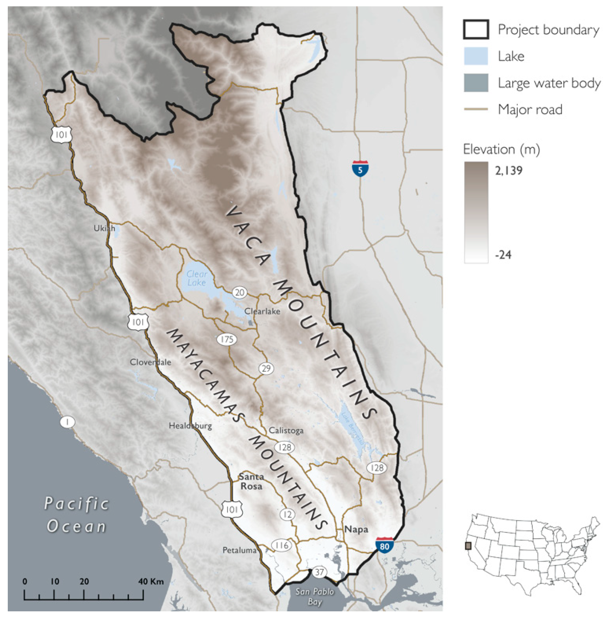
The project area (11,671 km2) included the inland region of the North Coast from 10 counties in Northern California: Colusa, Glenn, Lake, Marin, Mendocino, Napa, Solano, Sonoma, Tehama, and Yolo (centroid: 529,504 m, 4,315,244 m; north: 4,412,694 m, south: 4,214,915 m, east: 584,757 m, west: 459,722 m; NAD 1983 UTM Zone 10N) (Figure 1). The project area was delineated using a combination of three landscape features: watersheds (HUC8), primary roads, and elevation (>100 m).
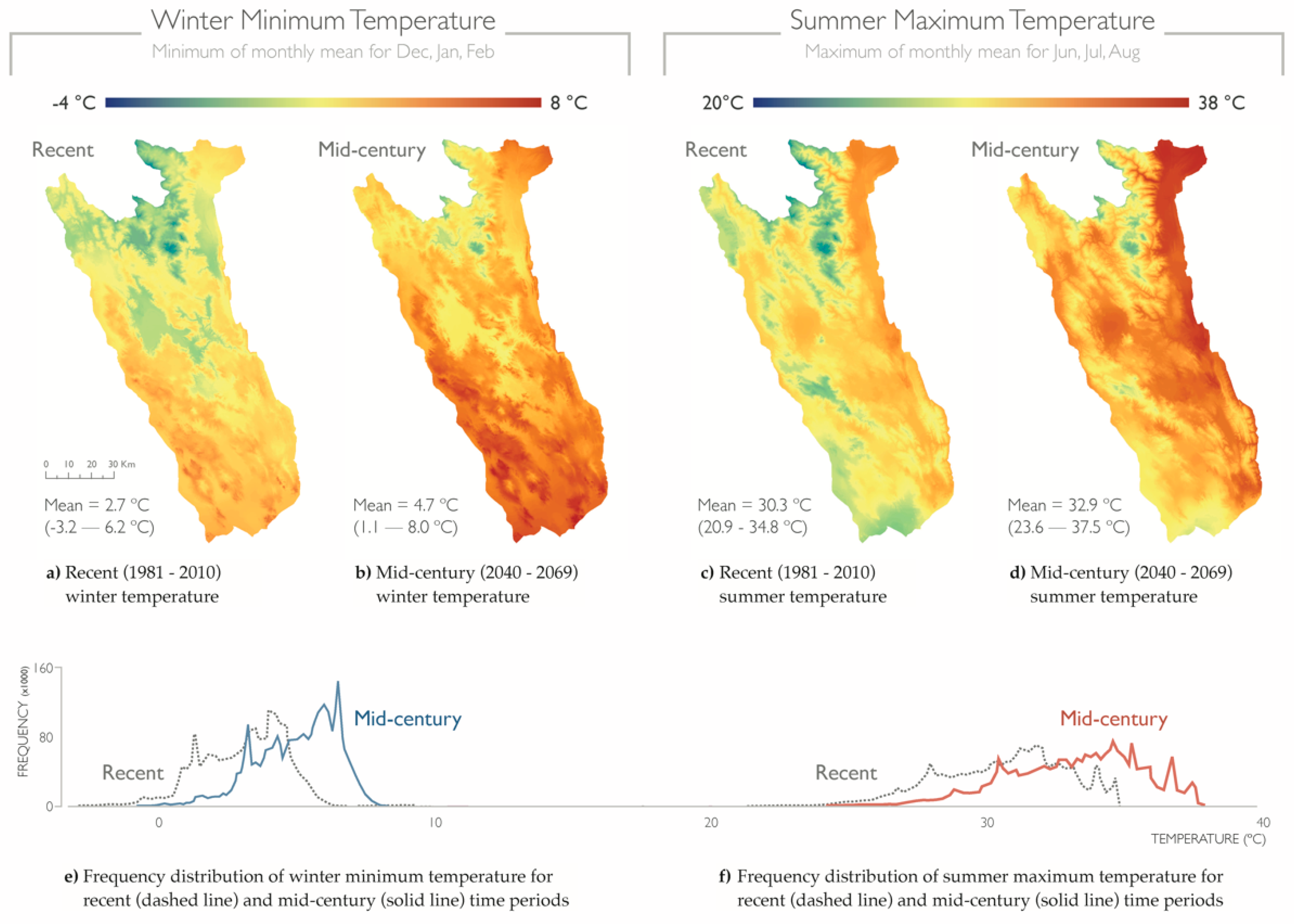
Located within a Mediterranean-climate region, as well as in the California Floristic Province—one of 25 global biodiversity hotspots that provides critical habitat for 584 vertebrates and 2125 endemic plants [71] —the project area was characterized by hot dry summers (mean = 30.3 °C, range: 20.9–34.8 °C; 1981–2010 30 y average), and mild, wet winters (average mean = 2.7 °C, range: −3.2–6.2 °C; 1981–2010 30 y average) [77]). Elevations ranged from −24 m to 2139 m. The four primary land cover types within the project area were (1) forest and woodland (46%), (2) shrubland and grassland (40%), (3) agricultural land (6%, maximum of 13% in Napa County), and (4) land that is developed or otherwise of human use (4%) [78]. The study area included the cities of Napa, Santa Rosa, Petaluma, Healdsburg, Clearlake, and Ukiah, and had a greater percent of privately-owned lands than what is observed statewide (study area = 60%, California = 51%) [79,80]. PAs comprised 40% of the project area (6961 km2) [79,80].
2.2. Terrestrial and Riparian Connectivity
For the connectivity evaluation, our aim was to identify broad regions of habitat that have the potential to facilitate the movement of multiple species and maintain ecological processes. We evaluated terrestrial and riparian connectivity and predicted optimal linkages to connect habitat patches using a node-based method to identify potential connections between existing PAs. First, we generated 302 node polygons to use as input for subsequent linkage assessment. Nodes were created using PA locations collated from the California Protected Area Database [79] and the California Conservation Easement Database [80] that were amended to include additional properties managed by participating stakeholders. We dissolved the boundaries between all contiguous PAs and excluded properties smaller than 200 m2 (~50 acres), resulting in a final set of polygons (i.e., nodes) that included lands owned in fee and protected for open space purposes, as well as those protected under conservation easements. All spatial analyses were conducted using ArcGIS 10.4.1 software [81].
Next, we used Linkage Mapper to create cost-weighted distance maps and least cost paths (LCPs) between perimeters of up to three PA nodes [82]. Linkage Mapper is a computer program that maps the linkages across the landscape among user-defined nodes of habitat, such as PAs. The resulting linkages show the relative value of each grid cell in providing connectivity. Each linkage contains a least cost path, which is the pathway between nodes that encounters the fewest features that impede movement. Model input parameters were set to construct a network of nodes using cost-weighted and Euclidean distance, exclude connections that intersected nodes, and prune the network using a maximum of three connected nearest neighbors using cost-weighted distance as the measurement unit. Final linkages were clipped to exclude PA locations and visualized using a threshold cost-weighted distance.
As a cost surface for the terrestrial connectivity linkages, we used an approximation of the degree of human modification that was based on stressors such as land use, land cover, as well as the presence of, use of, and distance from roads [50] (raster data for human modification at 30 m2 resolution provided by The Nature Conservancy). We opted to use the generous cost-weighted distance threshold of 25 km for terrestrial linkages because making connections as wide as possible is a simple way to ensure they contain a diverse topography that provides micro-refugial sites for species persistence [83].
For the riparian connectivity linkages, a resistance surface at 30 m2 resolution was created based on a terrain ruggedness index [84]. The surface was modified to include topographically defined creek features, and two landform types (valley bottom and narrow valley bottom) to represent landscape features with zero cost for terrestrial wildlife movement [40]. Linkage Mapper was used to generate least cost paths (LCP) and linkages between perimeters of adjacent PAs to show the most cost-effective route between a source and PA destinations. We visualized riparian linkages using a threshold cost-weighted distance of 1 km to evaluate the influence of these features at a local scale.
Terrestrial and riparian permeability estimates were calculated using the inverse of each resistance surface.
2.3. Cooling Benefit for Seasonal Temperature Extremes
We calculate the maximum net difference between the temperatures at two locations within a designated area as the cooling benefit and report these results in degrees temperature. For example, the cooling benefit afforded by a linkage that connects a pair of PAs with the same temperature is 0 °C. For PA pairs with unequal temperatures, the linkage will provide the warmer PA with access to the lower temperatures found within the cooler PA. Because using high-resolution climate and hydrological data in conservation planning improves the likely resilience of biodiversity to climate change [35], we conducted all climate and connectivity analyses using raster data at 30 m2 resolution.
We calculated the potential cooling benefit provided by each linkage between recent (1981–2010) and mid-century (2040–2069) time periods using the CNRM-CM5 [85] (Centre National de Recherches Météorologiques; Centre Européen de Recherche et Formation Avancée) general circulation model (under the representative concentration pathway (RCP) 8.5 emission scenario [86], a model predicting an “intermediate” future climate space Given the nuanced influence of temperature in California’s ecosystem and economy, we evaluated mean summer maximum (average of June, July, and August means (JJA)) and mean winter minimum (average of December, January, February means (DJF)) temperatures. The Basin Characterization Model (BCM) models the interactions of climate (e.g., rainfall and temperature) with empirically measured landscape attributes including topography, soils, and underlying geology [77]. This dataset provides historical and projected climate and hydrologic surfaces for the region. The BCM uses a minimum time step of monthly results at a resolution of 30 m2, allowing the generation of scenarios at annual, seasonal, or monthly time steps.
We extrapolated the model results across the project area to visualize the distribution of each temperature variable under recent and mid-century time periods. To compare the temperature distribution between the recent and mid-century time points, we divided the temperature values into 0.25 °C increments, calculated the number of cells in each 0.25 °C increment, and generated abundance plots. Lastly, we generated summary statistics for each temperature variable.
We quantified the maximum temperature benefit added to each PA by maintaining a linkage with a neighboring PA using net cooling as an indicator of resilience to climate change. We considered the linkage area unsuitable for permanent habitat, so climate benefits were only realized by connecting to a PA. Consequently, we did not consider the values within the linkage when calculating the final benefit of connecting two PAs. To calculate the maximum cooling benefit for each linkage, we found the difference between the lowest grid cell values for each temperature variable (i.e., minimum temperature) for all PAs connected by a linkage. This value represented the maximum net cooling the network presents over any one individual PA. We assigned this value to the adjoining linkage to represent the added benefit of the network in maintaining access to cooler temperatures.
To account for a bias toward lower minimum temperatures in large PAs that may not be realistically accessible from a linkage, we corrected for size differences by restricting the search area used for obtaining a minimum temperature within PAs greater than 5 km2. Rather than taking the absolute minimum temperature for the entire PA, we restricted the climate benefit calculation to use the minimum temperature within a 5 km2 radius around the linkage-PA connection point. This radius was used as an approximation of the potential dispersal distance for a medium mammal into a PA.
3. Results
3.1. Terrestrial and Riparian Connectivity
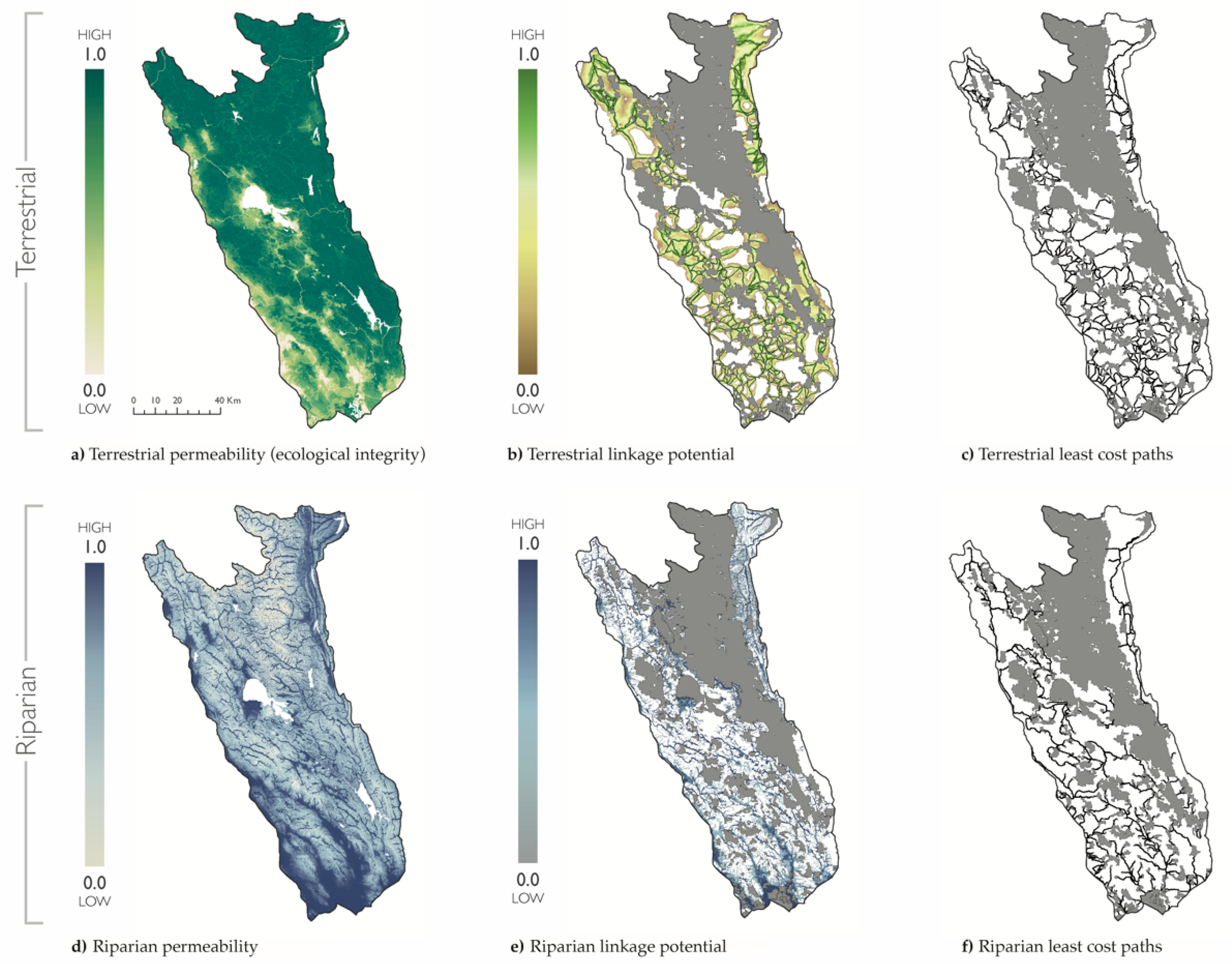
Mean terrestrial permeability was 0.78 for the project area (range: <0.01–1.00), and 0.84 within terrestrial linkages (range: <0.01–1.00) (Figure 2). Human modification was greatest in the southwest region and along the western boundary, which was delimited by a major freeway (U.S. 101). Mean riparian permeability was 0.81 for the project area (range: 0.00–1.00), and 0.93 within riparian linkages (range: 0.33–1.00). Riparian permeability was greatest in the southern part of the study region near the tidal estuary of San Pablo Bay, CA. Mountain peaks and steep slopes had the lowest values of riparian permeability.
The terrestrial connectivity assessment resulted in 660 broad linkages, with a mean length of 3.22 km (range: 0.09–47.13 km). Linkage length and width increased with the underlying landscape permeability and distance between PAs. Specifically, connections were narrow and short in the more developed southern region, where PAs were smaller in size and closer together. In contrast, linkages were wider and longer in more remote locations where PAs were larger, and the habitat was highly permeable. The longest linkages were located at the periphery of the project area, connecting small PAs across long distances to the PA network. The total area of all terrestrial linkages covered 56% of the project area (6526 km2).
The riparian linkage assessment resulted in 497 thin linkages, with a mean length of 11.26 km (range: 0.03–110.06 km). Overall, linkage length and width were narrow, although wider linkages were found in wetland and lowland areas with high riparian permeability. The total area of all riparian linkages covered 38% of the project area (4465 km2). Riparian linkages were closer to streets and roads than terrestrial linkages. A Mann-Whitney U test showed that there was a significant difference (W = 109,032, p-value = 8.51 × 10⁻¹⁶) between distance to streets and roads for riparian linkages when compared with terrestrial linkages. The median distance was 212 m for riparian linkages (mean = 377.36 m; range: 0.00–5819.75 m) compared to 359 m for terrestrial linkages (mean = 549.77 m; range: 7.50–6481.11 m).
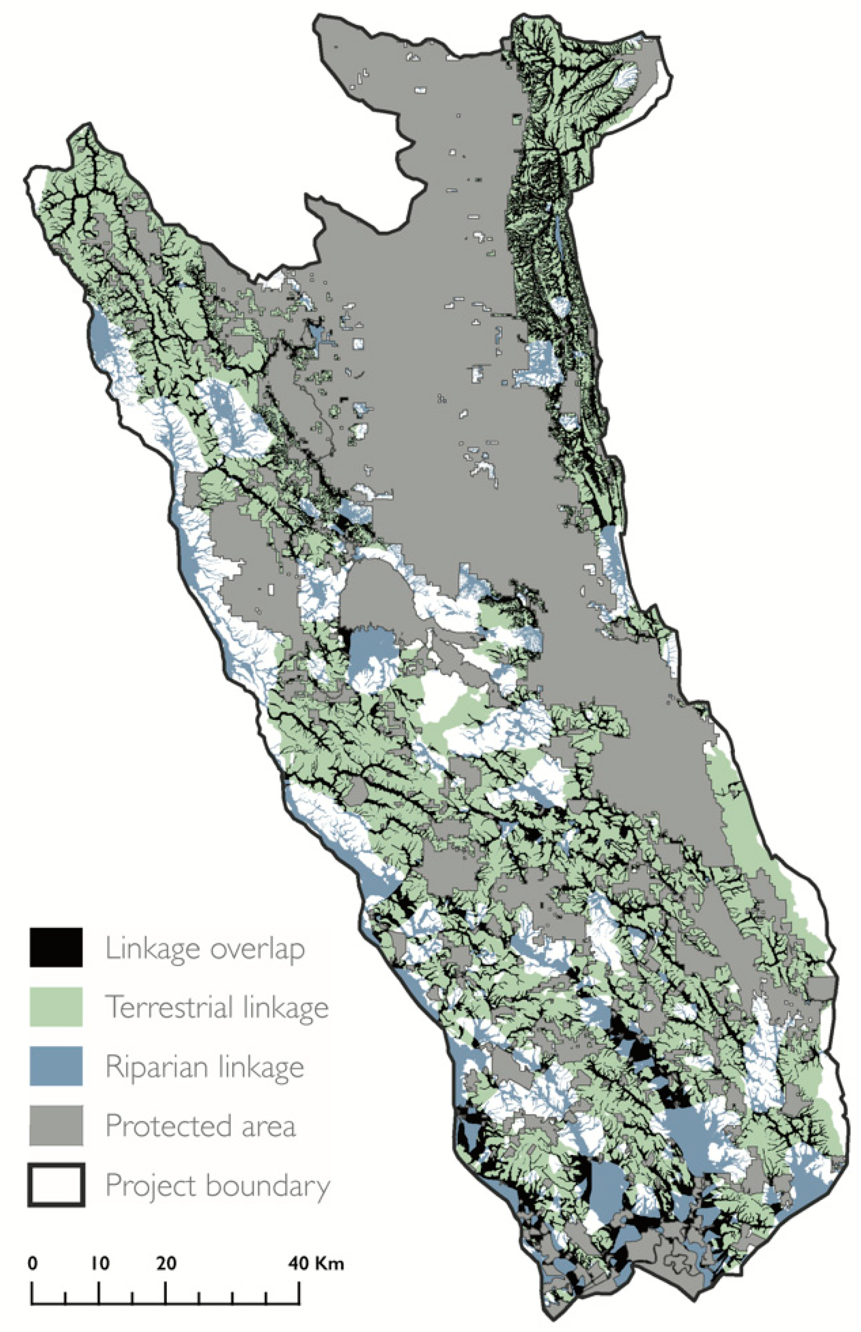
Terrestrial and riparian linkages showed distinct spatial patterns. Terrestrial linkage orientation was primarily east to west, avoided cities, and increased in density with distance from major roads. Riparian linkages had a distinct north–south orientation, and overlapped with major roads, which also follow topography across valley bottoms. As a result, the two linkage types were roughly perpendicular to each other. We found little overlap between the terrestrial and riparian linkages (Figure 3). The total overlap between the terrestrial and riparian linkages overlapped comprised 19% of the project area (2173 km2). The widest areas of overlap to the southwest. This region contained many terrestrial linkages between numerous small PAs, and expansive riparian linkages following the valley bottoms and lowland area near San Pablo Bay.
3.2. Cooling Benefit for Seasonal Temperature Extremes
Temperature increased between recent and mid-century time periods for both summer and winter variables (Figure 4). Seasonal extreme temperatures showed distinct temperature and spatial distribution profiles. The coolest and hottest locations for each variable were consistent across time periods, although the average temperature at these sites was +2.3 °C warmer at mid-century. Specifically, the warmest locations in winter were coastal lowlands to the southwest of the project area, whereas inland valleys were warmest for summer. The average change between current and future was +2.6 °C for mean summer maximum (range: 1.3–4.2 °C), and +2.0 °C (range: 0.4–3.2 °C) for mean winter minimum temperature.
Although the coolest and warmest locations were consistent within each variable, these locations differed between summer and winter temperature projections. The coolest locations were concentrated at the high elevations to the north of the project area during winter months and distributed across the southern lowlands and throughout the western region closest to the coast for summer months. The warmest locations were in the south and coastward for winter, and in valleys and lowlands for summer.
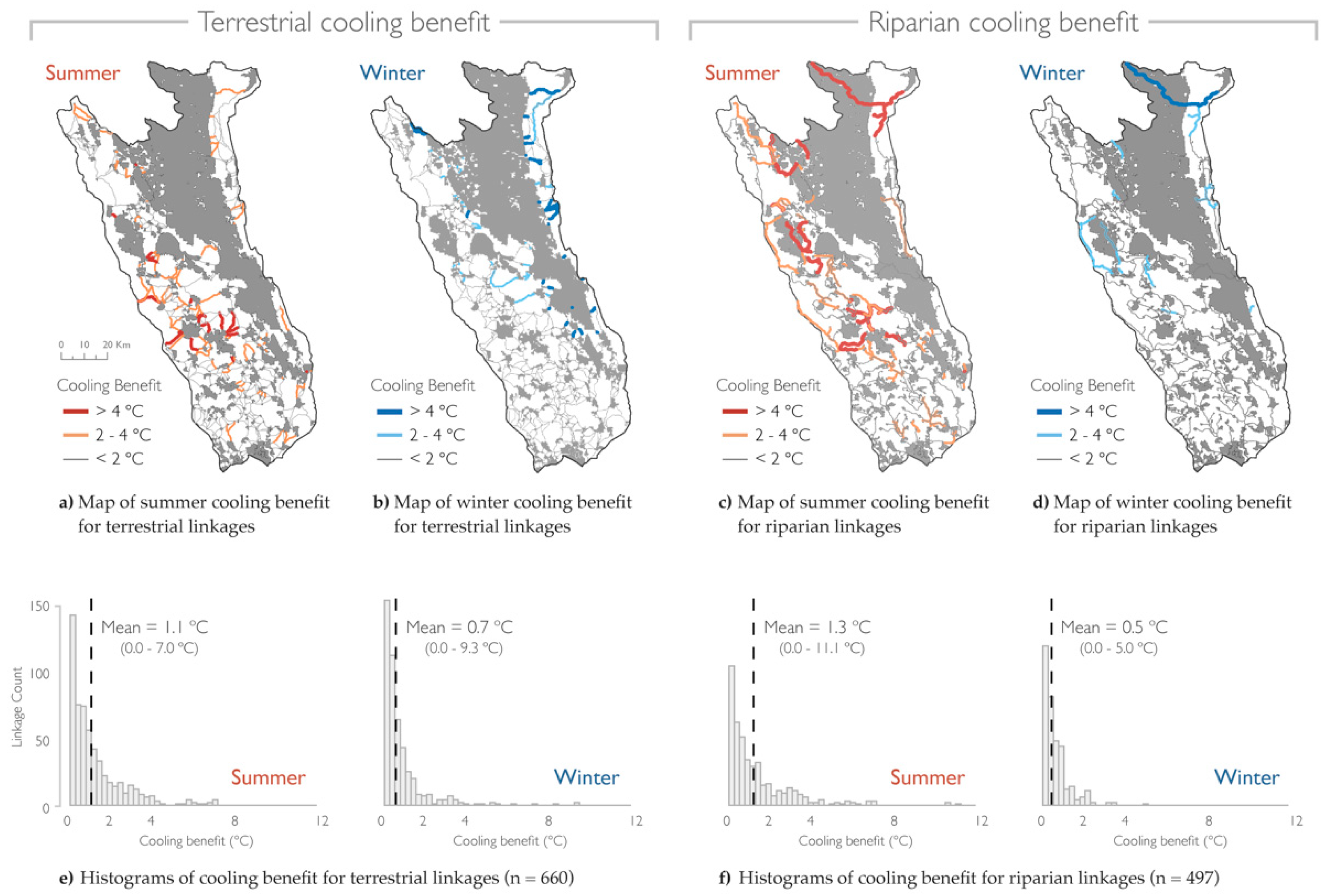
Terrestrial and riparian linkages were projected to offer greater cooling benefits for summer when compared to winter. (Figure 5). The median of the maximum cooling benefit for terrestrial linkages was 0.70 °C (mean = 1.12 °C) for summer compared to 0.36 °C (mean = 0.67 °C) for winter. The median of the maximum cooling benefit for riparian linkages was 0.72 °C (mean = 1.27 °C) for summer compared to 0.32 °C (mean = 0.52 °C) for winter. A Mann–Whitney U test showed that there was a significant difference (W = 7964, p = 0.02) between cooling benefit for summer when compared to winter for both terrestrial (W = 279,188, p-value < 2.20 × 10⁻¹⁶) and riparian (W = 167,851, p-value < 2.20 × 10⁻¹⁶) linkages.
The spatial distribution of the linkages with the greatest cooling benefit (>4 °C) showed a consistent contrast between summer and winter for terrestrial and riparian connectivity. For both linkage types, the greatest cooling benefit was observed in the west for summer and in the northeast for winter. We observed intra-seasonal differences in the spatial distribution of the greatest cooling benefit between the two linkage types. This difference was most pronounced for summer cooling projections. Terrestrial linkages with the greatest cooling benefit were more clustered into specific geographic regions. In contrast, riparian linkages provided high levels of cooling across a larger extent that included the northwest and northeast of the project area.
4. Discussion
4.1. Terrestrial and Riparian Connectivity
The distinct spatial patterns presented by the terrestrial and riparian linkages offer two complementary options for enhancing connectivity through human-modified landscapes. The perpendicular configuration of the two linkage types approximates a lattice-work corridor, which is composed of an interconnected network of riparian linkages and perpendicular elevational bands designed to address both dispersal and persistence in the context of climate change [87]. Locations where terrestrial and riparian linkages overlap represent areas with connectivity co-benefits, and we recommend prioritizing the evaluation of these areas for protection.
We used a node-based method based on stakeholder input during methods development to identify priority areas for connectivity among PAs that they are responsible for the management of. A node-less approach can be done using OmniScape to generate a continuous connectivity surface using a moving window to calculate multiple flow paths of least resistance across the landscape [88]. The Nature Conservancy’s Omniscape connectivity data [89] was generated using the same index of ecological integrity that informed the terrestrial linkages we generated here [50]. A post-hoc comparison between our terrestrial linkages and locations prioritized by Omniscape showed very similar results. A more quantitative comparison of node-based and omnidirectional connectivity priorities could provide insight about their strengths and weaknesses that may be used to inform model selection in future connectivity assessments.
Although species-agnostic structural models may be better suited for addressing landscape resilience for multiple ecosystems, a focal-species approach is important to consider for conservation management [90]. We used structural connectivity models to generate regional maps of terrestrial and riparian linkages intended for use by stakeholders to guide local priority setting for corridor implementation. The work presented here was co-produced as part of a multi-jurisdictional practitioner network using a framework that provided facilitated and sustained stakeholder engagement [73]. Because stakeholders were directly involved in the climate-wise connectivity assessment, we were able to emphasize the conceptual difference between these perspectives in connectivity modeling, as well as the potential and limitations of resulting maps. In particular, it is widely appreciated that potential linkages predicted by structural connectivity models require validation [91]. For example, two evaluations of the functional connectivity of the linkages generated here are currently ongoing to evaluate the movement of wide-ranging terrestrial mammals using genetic and telemetry methods.
The approach we used identified terrestrial linkages using existing land-use and land-cover data; however, these locations may not persist as viable connections into the future. Land conversion and fragmentation are associated with increases in human population worldwide [17]. Urban expansion around PAs is projected to expand by 67% under business-as-usual conditions [92]. Because range shifts due to climate change could result in species moving beyond PA boundaries, static PA networks may be unable to provide suitable conditions in the future [93,94,95]. Few scenarios of future climate change have modeled projected-land use patterns (e.g., land conversion and fragmentation) that will reduce habitat for species persistence [96,97]. Consequently, there is a need to explore the interaction between changing land use and climate in climate connectivity analyses. For example, a comparison of connectivity predictions using existing and projected future land use could improve the long-term function of PA networks.
4.2. Cooling Benefit for Seasonal Temperature Extremes
Our results showed large differences in temperature temporally, between current and future climate, and spatially, between neighboring PAs. There are also clear seasonal differences between the spatial trends, strength, and orientation of cooling benefit for both terrestrial and riparian linkages. The spatial distribution of the linkages with the greatest cooling benefit (>4 °C) showed a consistent contrast between summer and winter for both terrestrial and riparian connectivity. Overall, cooler summer temperatures were found in the western portion of the project area closer to the coast, whereas the cooler winter temperatures were found inland to the east. For both linkage types, the greatest cooling benefit was observed in the west for summer and in the northeast, toward higher latitude and elevation, for winter. The latter is more consistent with observed species range shifts and the working paradigm that species limited by warmer temperatures will move upload and to cooler latitudes. The former then represents a lesser appreciated phenomenon that is likely to be relevant for other coastal regions.
These insights into locations that offer seasonal cooling has the potential to advance species-informed climate-wise conservation planning. Observed temperature-driven responses to climate change—such as shifts in phenology, species abundance, and community diversity—have a clear seasonal component. For example, warmer winter temperatures are expected to lead to the tropicalization of temperate ecosystems, where cold-intolerant species expand poleward in response to shorter, milder freezing events [98]. Increases in summer maximum temperatures are expected to increase the frequency of heat stress and negatively impact the fitness of many species, especially ectotherms [99]. Using the minimum temperature found within each PA provides the maximum cooling benefit. An alternative approach could include the mean or median temperature within each PA, and future work could include a sensitivity analysis to compare results calculated using these metrics.
We recognize the challenges of selecting climate metrics and models, owing to the numerous variables that measure different aspects of climate as well as variability in projections depending on the time period and emissions scenario used in their creation. The approach we used to evaluate cooling benefit considered one climate metric and one climate model. We restricted our analysis to an assessment of temperature based on the availability of data with the sufficient spatial and temporal resolution to assess the influence of fine-scale landscape features and seasonal trends on cooling benefit. The assessment could be improved by including additional climate metrics, such as seasonal precipitation patterns. Although precipitation is an important driver of climate space in Mediterranean regions, it was excluded here because we lacked data with the spatial and temporal resolution needed to account for the highly variable precipitation in California [100]. The analysis could also be improved by addressing climate model uncertainty, such as testing the influence of multiple climate models or future time periods on the magnitude and direction of cooling benefit. Because the overarching goal of the climate connectivity assessment was to develop tools that would enhance land management decisions, we elected to use a single climate metric to focus the assessment and decrease the number of resulting data products. At the outset of the project we evaluated three climate models (CCSM4 [101] (Community Climate System Model), CNRM-CM5, and MIROC-ESM [102] (Model for Interdisciplinary Research on Climate – Earth System Model), and selected the CNRM-CM5 model to identify potential cooling benefits under an intermediate future scenario.
The juxtaposed orientation observed between terrestrial and riparian linkages creates an intersecting framework that may be used to identify priority cooling pathways across and between elevational bands. The north–south connectivity in the riparian linkages provided hot lowland areas access to cooler high-elevation habitat, and the east–west connectivity of the terrestrial linkages across an elevational band provided hot interior lands access to cooler coastal habitat.
5. Conclusions
Delineating both terrestrial and riparian linkages revealed distinct spatial patterns between the linkage types and offers two complementary options for enhancing connectivity through human-modified landscapes. In particular, protecting riparian corridors that are already used for animal and plant movement, especially in the long dry season, may prove to be the most effective implementation strategy. Riparian zones already have some legal protection in many places [38], and humans often support the conservation of riparian areas for the key ecosystem services provided by healthy rivers and streams [87]. Financial incentives are also available to agricultural landowners for the protection of soil and freshwater resources these areas provide.
Quantifying the cooling benefits of both terrestrial and riparian linkages allowed the conservation practitioners we work with to prioritize their conservation actions (e.g., acquisition, restoration, corridor planning and implementation) on climate resilience, as well as habitat connectivity [75]. For example, these methods have been used to generate six corridor reports that provide regional- and parcel-scale data for a suite of connectivity and climate metrics, identify key information and data gaps, specify critical partners, and identify next steps for corridor implementation. The parcel-by-parcel estimates of terrestrial and climate connectivity have already been used by land managers in the U.S. Bureau of Land Management, Land Trust of Napa County, and Sonoma Land Trust to prioritize conservation plans and investments. A companion statewide evaluation of additional future scenarios will provide the opportunity to explore how spatial trends and climate benefit predictions for seasonal temperatures interact beyond this Coast Ranges study area.
Paired with mid-century projections, an evaluation of seasonal influence of temperature on linkage cooling benefit demonstrated distinct trends for summer and winter variables. This approach can improve connectivity planning for biodiversity conservation in Mediterranean-type landscapes world-wide, where observed temperature-driven responses to climate have a clear seasonal component [70]. Thus, in locations with topoclimate diversity or ocean climate influence, evaluating seasonal temperatures independently is required to assess climate refugia and climate-wise connectivity.
In sum, delineating both riparian and terrestrial structural linkages, and prioritizing these linkages based on their cooling benefit during winter and summer, provides essential spatial planning information to protect landscape-scale climate resilience.
Author Contributions
Conceptualization, A.M., E.M. and M.G.; methodology, A.M., E.M. and M.G.; software, M.G.; validation, M.G.; formal analysis, M.G. and A.M.; investigation, A.M., E.M. and M.G.; resources, E.M. and A.M.; data curation, M.G. and T.C.; writing—original draft preparation, M.G.; writing—review and editing, M.G., A.M., E.M. and T.C.; visualization, M.G.; supervision, A.M., E.M. and T.C.; project administration, E.M. and T.C.; funding acquisition, A.M. and E.M. All authors have read and agreed to the published version of the manuscript.
Funding
This research was funded by California Landscape Conservation Partnership, Cooperative Agreement: F16AC00574 and by Pepperwood Foundation donors.
Acknowledgments
The authors thank TBC3 colleagues L.E. Flint and A.L. Flint (United States Geological Survey) for assistance with downscaling of climate projections derived from the California Basin Characterization Model, and S.B. Weiss for the topoclimate concept. Gratitude goes to the Mayacamas to Berryessa Connectivity Network’s steering committee who participated in the co-creation of these methods and project outputs: S. Adams, M. Cooper and J. Wirka (Audubon Canyon Ranch); K. Barnitz and J. Weigand (United States Bureau of Land Management); C.E. Koehler (Lake County Land Trust and McLaughlin Preserve); T.R. Smythe (Lake County Land Trust); M. Palladini (Land Trust of Napa County); K.A. Gaffney, A. Roa, and A. Schichtel (Sonoma County Ag + Open Space); H. Brown (Sonoma County Regional Parks); and W. Eliot, T. George, A. Johnston, and T. Nelson (Sonoma Land Trust).
Conflicts of Interest
The authors declare no conflict of interest. The funders had no role in the design of the study; in the collection, analyses, or interpretation of data; in the writing of the manuscript, or in the decision to publish the results.
References
- Pecl, G.T.; Araújo, M.B.; Bell, J.D.; Blanchard, J.; Bonebrake, T.C.; Chen, I.-C.; Clark, T.D.; Colwell, R.K.; Danielsen, F.; Evengård, B.; et al. (Supplement) Biodiversity redistribution under climate change: Impacts on ecosystems and human well-being. Science 2017, 355. [Google Scholar] [CrossRef]
- Berg, M.P.; Toby Kiers, E.; Driessen, G.; van der Heijden, M.; Kooi, B.W.; Kuenen, F.; Liefting, M.; Verhoef, H.A.; Ellers, J. Adapt or disperse: Understanding species persistence in a changing world. Glob. Chang. Biol. 2010, 16, 587–598. [Google Scholar] [CrossRef]
- Krosby, M.; Tewksbury, J.; Haddad, N.; Hoekstra, J. Ecological Connectivity for a Changing Climate. Conserv. Biol. 2010, 24, 1686–1689. [Google Scholar] [CrossRef] [PubMed]
- Burrows, M.T.; Schoeman, D.S.; Richardson, A.J.; Molinos, J.G.; Hoffmann, A.; Buckley, L.B.; Moore, P.J.; Brown, C.J.; Bruno, J.F.; Duarte, C.M.; et al. Geographical limits to species-range shifts are suggested by climate velocity. Nature 2014, 507, 492–495. [Google Scholar] [CrossRef]
- Chen, I.; Hill, J.K.; Ohlemüller, R.; Roy, D.B.; Thomas, C.D. Rapid Range Shifts of Species Associated with High Levels of Climate Warming. Science 2011, 333, 1024–1026. [Google Scholar] [CrossRef]
- Hickling, R.; Roy, D.B.; Hill, J.K.; Fox, R.; Thomas, C.D. The distributions of a wide range of taxonomic groups are expanding polewards. Glob. Chang. Biol. 2006, 12, 450–455. [Google Scholar] [CrossRef]
- Fei, S.; Desprez, J.M.; Potter, K.M.; Jo, I.; Knott, J.A.; Oswalt, C.M. Divergence of species responses to climate change. Sci. Adv. 2017, 3, e1603055. [Google Scholar] [CrossRef] [Green Version]
- Moritz, C.; Patton, J.L.; Conroy, C.J.; Parra, J.L.; White, G.C.; Beissinger, S.R. Impact of a Century of Climate Change on Small-Mammal Communities in Yosemite National Park, USA. Science 2008, 322, 261–264. [Google Scholar] [CrossRef] [Green Version]
- Tingley, M.W.; Koo, M.S.; Moritz, C.; Rush, A.C.; Beissinger, S.R. The push and pull of climate change causes heterogeneous shifts in avian elevational ranges. Glob. Chang. Biol. 2012, 18, 3279–3290. [Google Scholar] [CrossRef]
- Roelke, M.E.; Martenson, J.S.; O’Brien, S.J.; Jablonski, D.; Stanley, S.M.; Myers, N.; Elliot, D.K.; Centre, T.I.C.M.; Service, U.S.F.W.; Service, U.S.F.W.; et al. The consequences of demographic reduction and genetic depletion in the endangered Florida panther. Curr. Biol. 1993, 3, 340–350. [Google Scholar] [CrossRef]
- Fahrig, L.; Merriam, G. Conservation of fragmented populations. Conserv. Biol. 1994, 8, 50–59. [Google Scholar] [CrossRef] [Green Version]
- Epps, C.W.; Palsbøll, P.J.; Wehausen, J.D.; Roderick, G.K.; Ramey, R.R.; McCullough, D.R. Highways block gene flow and cause a rapid decline in genetic diversity of desert bighorn sheep. Ecol. Lett. 2005, 8, 1029–1038. [Google Scholar] [CrossRef] [Green Version]
- Charlesworth, D.; Charlesworth, D.; Willis, J.H.; Willis, J.H. The genetics of inbreeding depression. Nat. Rev. Genet. 2009, 10, 783–796. [Google Scholar] [CrossRef]
- Hannah, L. Climate Change, Connectivity, and Conservation Success. Conserv. Biol. 2011, 25, 1139–1142. [Google Scholar] [CrossRef] [PubMed]
- Hilty, J.A.; Lidicker, W.Z.; Merenlender, A. Corridor Ecology: The Science and Practice of Linking Landscapes for Biodiversity Conservation; Island Press: Washington, DC, USA, 2006; ISBN 1597265934. [Google Scholar]
- Heller, N.; Zavaleta, E. Biodiversity management in the face of climate change: A review of 22 years of recommendations. Biol. Conserv. 2009, 142, 14–32. [Google Scholar] [CrossRef]
- Tilman, D.; Clark, M.; Williams, D.R.; Kimmel, K.; Polasky, S.; Packer, C. Future threats to biodiversity and pathways to their prevention. Nature 2017, 546, 73–81. [Google Scholar] [CrossRef] [PubMed]
- Jayadevan, A.; Nayak, R.; Karanth, K.K.; Krishnaswamy, J.; DeFries, R.; Karanth, K.U.; Vaidyanathan, S. Navigating paved paradise: Evaluating landscape permeability to movement for large mammals in two conservation priority landscapes in India. Biol. Conserv. 2020, 247, 108613. [Google Scholar] [CrossRef]
- Hilty, J.A.; Keeley, A.T.H.; Lidicker, W.Z.; Merenlender, A.M. Corridor Ecology: Linking Landscapes for Biodiversity Conservation and Climate Adaptation, 2nd ed.; Island Press: Washington, DC, USA, 2019. [Google Scholar]
- Keeley, A.; Ackerly, D.; Cameron, D.; Heller, N.; Huber, P.; Schloss, C.; Thorne, J.; Merenlender, A. New concepts, models, and assessments of climate-wise connectivity. Environ. Res. Lett. 2018, 13. [Google Scholar] [CrossRef]
- Phillips, S.J.; Williams, P.; Midgley, G.; Archer, A. Optimizing Dispersal Corridors for the Cape Proteaceae Using Network Flow. Ecol. Appl. 2008, 18, 1200–1211. [Google Scholar] [CrossRef]
- Lawler, J.J.; Ruesch, A.S.; Olden, J.D.; McRae, B.H. Projected climate-driven faunal movement routes. Ecol. Lett. 2013, 16, 1014–1022. [Google Scholar] [CrossRef]
- Alagador, D.; Cerdeira, J.O.; Araújo, M.B. Climate change, species range shifts and dispersal corridors: An evaluation of spatial conservation models. Methods Ecol. Evol. 2016, 7, 853–866. [Google Scholar] [CrossRef] [Green Version]
- Rose, N.-A.; Burton, P.J. Using bioclimatic envelopes to identify temporal corridors in support of conservation planning in a changing climate. For. Ecol. Manag. 2009, 258, S64–S74. [Google Scholar] [CrossRef]
- Pellatt, M.G.; Goring, S.J.; Bodtker, K.M.; Cannon, A.J. Using a down-scaled bioclimate envelope model to determine long-term temporal connectivity of garry oak (Quercus garryana) habitat in Western North America: Implications for protected area planning. Environ. Manag. 2012, 49, 802–815. [Google Scholar] [CrossRef] [PubMed]
- Loarie, S.R.; Duffy, P.B.; Hamilton, H.; Asner, G.P.; Field, C.B.; Ackerly, D.D. The velocity of climate change. Nature 2009, 462, 1052–1055. [Google Scholar] [CrossRef] [PubMed]
- McKelvey, K.S.; Copeland, J.P.; Schwartz, M.K.; Littell, J.S.; Aubry, K.B.; Squires, J.R.; Parks, S.A.; Elsner, M.M.; Mauger, G.S. Climate change predicted to shift wolverine distributions, connectivity, and dispersal corridors. Ecol. Appl. 2011, 21, 2882–2897. [Google Scholar] [CrossRef] [Green Version]
- Howard, T.; Schlesinger, M.D. Wildlife habitat connectivity in the changing climate of New York’s Hudson Valley. Available online: https://nyaspubs.onlinelibrary.wiley.com/doi/10.1111/nyas.12172 (accessed on 25 September 2020).
- Drake, J.C.; Griffis-Kyle, K.; McIntyre, N.E. Using nested connectivity models to resolve management conflicts of isolated water networks in the Sonoran Desert. Ecosphere 2017, 8. [Google Scholar] [CrossRef]
- Littlefield, C.E.; McRae, B.H.; Michalak, J.; Lawler, J.J.; Carroll, C. Connecting today’s climates to future analogs to facilitate species movement under climate change. Conserv. Biol. 2017, 1–31. [Google Scholar] [CrossRef]
- Pressey, R.L. Conservation Planning for a Changing Climate. 2007. Available online: https://researchonline.jcu.edu.au/25280/1/15948.pdf (accessed on 25 September 2020).
- Noss, R. Beyond Kyoto: Forest management in a time of rapid climate change. Conserv. Biol. 2001, 15, 578–590. [Google Scholar] [CrossRef]
- Rouget, M.; Cowling, R.M.; Lombard, A.T.; Knight, A.T.; Kerley, G.I.H. Designing Large-Scale Conservation Corridors for Pattern and Process. Conserv. Biol. 2006, 20, 549–561. [Google Scholar] [CrossRef]
- Morelli, T.L.; Daly, C.; Dobrowski, S.Z.; Dulen, D.M.; Ebersole, J.L.; Jackson, S.T.; Lundquist, J.D.; Millar, C.I.; Maher, S.P.; Monahan, W.B.; et al. Managing climate change refugia for climate adaptation. PLoS ONE 2016, 11. [Google Scholar] [CrossRef] [Green Version]
- Heller, N.E.; Kreitler, J.; Ackerly, D.D.; Weiss, S.B.; Recinos, A.; Branciforte, R.; Flint, L.E.; Flint, A.L.; Micheli, E. Targeting climate diversity in conservation planning to build resilience to climate change. Ecosphere 2015, 6, 65. [Google Scholar] [CrossRef]
- Keppel, G.; Van Niel, K.P.; Wardell-Johnson, G.W.; Yates, C.J.; Byrne, M.; Mucina, L.; Schut, A.G.T.; Hopper, S.D.; Franklin, S.E. Refugia: Identifying and understanding safe havens for biodiversity under climate change. Glob. Ecol. Biogeogr. 2012, 21, 393–404. [Google Scholar] [CrossRef]
- Anderson, M.G.; Barnett, A.; Clark, M.; Sheldon, A.O.; Prince, J.; Vickery, B. Resilient and Connected Landscapes for Terrestrial Conservation. Available online: https://easterndivision.s3.amazonaws.com/Resilient_and_Connected_Landscapes_For_Terrestial_Conservation.pdf (accessed on 25 September 2020).
- Fremier, A.K.; Kiparsky, M.; Gmur, S.; Aycrigg, J.; Craig, R.K.; Svancara, L.K.; Goble, D.D.; Cosens, B.; Davis, F.W.; Scott, J.M. A riparian conservation network for ecological resilience. Biol. Conserv. 2015, 191, 29–37. [Google Scholar] [CrossRef] [Green Version]
- Capon, S.; Nally, R. Mac; Davies, P.M. Riparian Ecosystems in the 21st Century: Hotspots for Climate Change Adaptation? Environmental Water Needs for the Fitzroy River View project An Integrated Approach for Assessing Vulnerability and Potential Adaptation Options for a Coastal Water Supply and Demand System Subject to Climatic and Non-Climatic Changes View project. Ecosystems 2013, 16, 359–381. [Google Scholar] [CrossRef]
- Theobald, D.M.; Harrison-Atlas, D.; Monahan, W.B.; Albano, C.M. Ecologically-relevant maps of landforms and physiographic diversity for climate adaptation planning. PLoS ONE 2015, 10, 1–17. [Google Scholar] [CrossRef] [Green Version]
- Jeong, S.; Kim, H.G.; Thorne, J.H.; Lee, H.; Cho, Y.H.; Lee, D.K.; Park, C.H.; Seo, C. Evaluating connectivity for two mid-sized mammals across modified riparian corridors with wildlife crossing monitoring and species distribution modeling. Glob. Ecol. Conserv. 2018, 16, e00485. [Google Scholar] [CrossRef]
- Dickson, B.; Jenness, J.; Beier, P. Influence of vegetation, topography, and roads on cougar movement in southern California. J. Wildl. Manag. 2005, 69, 262–276. [Google Scholar] [CrossRef]
- Gillies, C.S.; St. Clair, C.C. Riparian corridors enhance movement of a forest specialist bird in fragmented tropical forest. Proc. Natl. Acad. Sci. USA 2008, 105, 19774–19779. [Google Scholar] [CrossRef] [Green Version]
- Hilty, J.A.; Merenlender, A.M. Use of Riparian Corridors and Vineyards by Mammalian Predators in Northern California. Conserv. Biol. 2004, 18, 126–135. [Google Scholar] [CrossRef]
- Sabo, J.L.; Sponseller, R.; Dixon, M.; Gade, K.; Harms, T.; Heffernan, J.; Jani, A.; Katz, G.; Soykan, C.; Watts, J.; et al. Riparian zones increase regional species richness by harboring different, not more, species. Ecology 2005, 86, 56–62. [Google Scholar] [CrossRef]
- Naiman, R.J.; Decamps, H.; Pollock, M. The Role of Riparian Corridors in Maintaining Regional Biodiversity. Ecol. Appl. 1993, 3, 209–212. [Google Scholar] [CrossRef] [PubMed]
- Parrish, J.D.; Braun, D.P.; Unnasch, R.S. Are We Conserving What We Say We Are? Measuring Ecological Integrity within Protected Areas; Oxford Academic: Oxford, UK, 2003; Volume 53. [Google Scholar]
- Belote, T.R.; Dietz, M.S.; McRae, B.H.; Theobald, D.M.; McClure, M.L.; Hugh Irwin, G.; McKinley, P.S.; Gage, J.A.; Aplet, G.H. Identifying corridors among large protected areas in the United States. PLoS ONE 2016, 11, e0154223. [Google Scholar] [CrossRef] [PubMed] [Green Version]
- Belote, T.R.; Dietz, M.S.; Jenkins, C.N.; McKinley, P.S.; Irwin, G.H.; Fullman, T.J.; Leppi, J.C.; Aplet, G.H. Wild, connected, and diverse: Building a more resilient system of protected areas. Ecol. Appl. 2017, 27, 1050–1056. [Google Scholar] [CrossRef] [PubMed]
- Theobald, D.M. A general model to quantify ecological integrity for landscape assessments and US application. Landsc. Ecol. 2013, 28, 1859–1874. [Google Scholar] [CrossRef]
- Dickson, B.G.; Albano, C.M.; Anantharaman, R.; Beier, P.; Fargione, J.; Graves, T.A.; Gray, M.E.; Hall, K.R.; Lawler, J.J.; Leonard, P.B.; et al. Circuit-theory applications to connectivity science and conservation. Conserv. Biol. 2019, 33, 239–249. [Google Scholar] [CrossRef]
- Crooks, K.R.; Burdett, C.L.; Theobald, D.M.; King, S.R.B.; Di Marco, M.; Rondinini, C.; Boitani, L. Quantification of habitat fragmentation reveals extinction risk in terrestrial mammals. Proc. Natl. Acad. Sci. USA 2017, 114, 7635–7640. [Google Scholar] [CrossRef] [Green Version]
- McGuire, J.L.; Lawler, J.J.; McRae, B.H.; Nuñez, T.A.; Theobald, D.M. Achieving climate connectivity in a fragmented landscape. Proc. Natl. Acad. Sci. USA 2016, 113, 7195–7200. [Google Scholar] [CrossRef] [Green Version]
- Game, E.T.; Lipsett-Moore, G.; Saxon, E.; Peterson, N.; Sheppard, S. Incorporating climate change adaptation into national conservation assessments. Glob. Chang. Biol. 2011, 17, 3150–3160. [Google Scholar] [CrossRef]
- Ohlemüller, R.; Anderson, B.J.; Araújo, M.B.; Butchart, S.H.M.; Kudrna, O.; Ridgely, R.S.; Thomas, C.D. The coincidence of climatic and species rarity: High risk to small-range species from climate change. Biol. Lett. 2008, 4, 568–572. [Google Scholar] [CrossRef] [Green Version]
- Williams, J.W.; Jackson, S.T.; Kutzbach, J.E. Projected distributions of novel and disappearing climates by 2100 AD. Proc. Natl. Acad. Sci. USA 2007, 104, 5738–5742. [Google Scholar] [CrossRef] [Green Version]
- Wright, S.J.; Muller-Landau, H.; Schipper, J. The Future of Tropical Species on a Warmer Planet. Conserv. Biol. 2009, 23, 1418–1426. [Google Scholar] [CrossRef] [PubMed]
- Iwamura, T.; Guisan, A.; Wilson, K.A.; Possingham, H.P. How robust are global conservation priorities to climate change? Glob. Environ. Chang. 2013, 23, 1277–1284. [Google Scholar] [CrossRef]
- Watson, J.E.M.; Iwamura, T.; Butt, N. Mapping vulnerability and conservation adaptation strategies under climate change. Nat. Clim. Chang. 2013, 3, 989–994. [Google Scholar] [CrossRef]
- Morelli, T.L.; Smith, A.B.; Kastely, C.R.; Mastroserio, I.; Moritz, C.; Beissinger, S.R. Anthropogenic refugia ameliorate the severe climate-related decline of a montane mammal along its trailing edge. Proc. R. Soc. B Biol. Sci. 2012, 279, 4279–4286. [Google Scholar] [CrossRef] [PubMed] [Green Version]
- Williams, C.M.; Henry, H.A.; Sinclair, B.J. Cold truths: How winter drives responses of terrestrial organisms to climate change. Biol. Rev. 2015, 90, 214–235. [Google Scholar] [CrossRef] [Green Version]
- Dolanc, C.R.; Thorne, J.H.; Safford, H.D. Widespread shifts in the demographic structure of subalpine forests in the Sierra Nevada, California, 1934 to 2007. Glob. Ecol. Biogeogr. 2013, 22, 264–276. [Google Scholar] [CrossRef]
- Morelli, T.L.; Maher, S.P.; Lim, M.C.W.; Kastely, C.; Eastman, L.M.; Flint, L.E.; Flint, A.L.; Beissinger, S.R.; Moritz, C. Climate change refugia and habitat connectivity promote species persistence. Clim. Chang. Responses 2017, 4, 1–12. [Google Scholar] [CrossRef] [Green Version]
- Blondel, J.; Aronson, J.; Bodiou, J.; Boeuf, G. The Mediterranean Region: Biological Diversity in Space and Time; Oxford University Press: Oxford, UK, 2010. [Google Scholar]
- Zittis, G. Observed rainfall trends and precipitation uncertainty in the vicinity of the Mediterranean, Middle East and North Africa. Appl. Clim. 2018, 134, 1207–1230. [Google Scholar] [CrossRef]
- Cook, B.I.; Anchukaitis, K.J.; Touchan, R.; Meko, D.M.; Cook, E.R. Spatiotemporal drought variability in the mediterranean over the last 900 years. J. Geophys. Res. 2016, 121, 2060–2074. [Google Scholar] [CrossRef]
- Giorgi, F.; Lionello, P. Climate change projections for the Mediterranean region. Glob. Planet. Chang. 2008, 63, 90–104. [Google Scholar] [CrossRef]
- Lionello, P.; Scarascia, L. The relation between climate change in the Mediterranean region and global warming. Reg. Environ. Chang. 2018, 18, 1481–1493. [Google Scholar] [CrossRef]
- Western Regional Climate Center Western Regional Climate Center: California Climate Tracker. Available online: https://wrcc.dri.edu/Climate/Tracker/CA/ (accessed on 25 September 2020).
- Office of Environmental Health Hazard Assessment. Indicators of Climate Change in California; Office of Environmental Health Hazard Assessment: Sacramento, CA, USA, 2018. [Google Scholar]
- Myers, N.; Mittermeier, R.A.; Mittermeier, C.G.; da Fonseca, G.A.B.; Kent, J. Biodiversity hotspots for conservation priorities. Nature 2000, 403, 853–858. [Google Scholar] [CrossRef] [PubMed]
- Bay Area Open Space Council. The Conservation Lands Network 2.0 Report; Bay Area Open Space Council: Berkeley, CA, USA, 2019. [Google Scholar]
- Gray, M.; Micheli, E.R.; Comendant, T.; Merenlender, A.M. Sustained stakeholder engagement promotes use of co-produced climate-wise connectivity knowledge by a practitioner network. Land 2020. under review. [Google Scholar]
- Beier, P. Conceptualizing and designing corridors for climate change. Ecol. Restor. 2012, 30, 312–319. [Google Scholar] [CrossRef]
- Rouget, M.; Cowling, R.M.; Pressey, R.L.; Richardson, D.M. Identifying spatial components of ecological and evolutionary processes for regional conservation planning in the Cape Floristic Region, South Africa. Divers. Distrib. 2003, 9, 191–210. [Google Scholar] [CrossRef]
- Stella, J.C.; Rodríguez-González, P.M.; Dufour, S.; Bendix, J.; Stella, J.C.; Rodríguez-González, P.M.; Dufour, S.; Bendix, J. Riparian vegetation research in Mediterranean-climate regions: Common patterns, ecological processes, and considerations for management. Hydrobiologia 2013, 719, 291–315. [Google Scholar] [CrossRef]
- Flint, L.E.; Flint, A.L.; Thorne, J.H.; Boynton, R. Fine-scale hydrologic modeling for regional landscape applications: The California Basin Characterization Model development and performance. Ecol. Process. 2013, 2, 1–21. [Google Scholar] [CrossRef] [Green Version]
- California Department of Forestry and Fire Protection Vegetation (fveg)—CALFIRE FRAP. [ds1327]; CALFIRE FRAP: Sacramento, CA, USA, 2015. [Google Scholar]
- Greeninfo Network California Protected Areas Database (Version 2017a). 2017. Available online: https://www.lacounts.org/dataset/california-protected-areas-database-2017a (accessed on 25 September 2020).
- Greeninfo Network California Conservation Easement Database (Version 2016). 2016. Available online: https://www.greeninfo.org/work/project/cpad-the-california-protected-areas-database (accessed on 25 September 2020).
- Esri ArcGIS Pro, Version 10.4.1; 2016. Available online: https://desktop.arcgis.com/en/arcmap/10.4/get-started/setup/arcgis-desktop-quick-start-guide.htm (accessed on 25 September 2020).
- McRae, B.; Kavanagh, D. Linkage Mapper Connectivity Analysis Software. 2011. Available online: https://circuitscape.org/linkagemapper/ (accessed on 25 September 2020).
- Jewitt, D.; Goodman, P.S.; Erasmus, B.F.N.; O’Connor, T.G.; Witkowski, E.T.F. Planning for the Maintenance of Floristic Diversity in the Face of Land Cover and Climate Change. Environ. Manag. 2017, 59, 792–806. [Google Scholar] [CrossRef]
- Riley, S.J.; DeGloria, S.D.; Elliot, R. A Terrain Ruggedness Index that Quantifies Topographic Heterogeneity. Intermt. J. Sci. 1999, 5, 23–27. [Google Scholar]
- Voldoire, A.; Sanchez-Gomez, E.; Salas y Mélia, D.; Decharme, B.; Cassou, C.; Sénési, S.; Valcke, S.; Beau, I.; Alias, A.; Chevallier, M.; et al. The CNRM-CM5.1 global climate model: Description and basic evaluation. Clim. Dyn. 2013, 40, 2091–2121. [Google Scholar] [CrossRef]
- Riahi, K.; Rao, S.; Krey, V.; Cho, C.; Chirkov, V.; Fischer, G.; Kindermann, G.; Nakicenovic, N.; Rafaj, P. RCP 8.5-A scenario of comparatively high greenhouse gas emissions. Clim. Chang. 2011, 109, 33–57. [Google Scholar] [CrossRef] [Green Version]
- Townsend, P.; Masters, K.L.; Townsend, P.A.; Masters, K.L. Lattice-work corridors for climate change: A conceptual framework for biodiversity conservation and social-ecological resilience in a tropical elevational gradient. Ecol. Soc. 2015. [Google Scholar] [CrossRef] [Green Version]
- McRae, B.H.; Popper, K.; Jones, A.; Schindel, M.; Buttrick, S.; Hall, K.R.; Unnasch, B.; Platt, J.; Unnasch, R.S.; Platt, J. Conserving Nature’s Stage: Mapping Omnidirectional Connectivity for Resilient Terrestrial Landscapes in the Pacific Northwest; The Nature Conservancy: Portland, OR, USA, 2016; p. 47. [Google Scholar] [CrossRef]
- The Nature Conservancy Omniscape 2018. Available online: https://omniscape.codefornature.org/ (accessed on 25 September 2020).
- Marrec, R.; Abdel Moniem, H.; Iravani, M.; Hricko, B.; Kariyeva, J.; Wagner, H.H. Conceptual framework and uncertainty analysis for large-scale, species-agnostic modelling of landscape connectivity across Alberta, Canada. Sci. Rep. 2020, 10. [Google Scholar] [CrossRef] [PubMed] [Green Version]
- Brown, E.D.; Williams, B.K.; Hodges, K.E.; Gov, E. Ecological integrity assessment as a metric of biodiversity: Are we measuring what we say we are? Biodivers. Conserv. 2016, 25, 1011–1035. [Google Scholar] [CrossRef] [Green Version]
- Martinuzzi, S.S.; Radeloff, V.C.; Joppa, L.N.; Hamilton, C.M.; Helmers, D.P.; Plantinga, A.J.; Lewis, D.J. Scenarios of future land use change around United States’ protected areas. Biol. Conserv. 2015, 184, 446–455. [Google Scholar] [CrossRef]
- Klausmeyer, K.R.; Shaw, M.R. Climate change, habitat loss, protected areas and the climate adaptation potential of species in Mediterranean ecosystems wordwide. PLoS ONE 2009, 4, 1–9. [Google Scholar] [CrossRef] [Green Version]
- Araújo, M.B.; Alagador, D.; Cabeza, M.; Nogués-Bravo, D.; Thuiller, W. Climate change threatens European conservation areas. Ecol. Lett. 2011, 14, 484–492. [Google Scholar] [CrossRef] [Green Version]
- Regos, A.; D’Amen, M.; Titeux, N.; Herrando, S.; Guisan, A.; Brotons, L. Predicting the future effectiveness of protected areas for bird conservation in Mediterranean ecosystems under climate change and novel fire regime scenarios. Divers. Distrib. 2016, 22, 83–96. [Google Scholar] [CrossRef]
- Jetz, W.; Wilcove, D.S.; Dobson, A.P. Projected impacts of climate and land-use change on the global diversity of birds. PLoS Biol. 2007, 5, 1211–1219. [Google Scholar] [CrossRef] [Green Version]
- Elsen, P.R.; Monahan, W.B.; Merenlender, A.M. Topography and human pressure in mountain ranges alter expected species responses to climate change. Nat. Commun. 2020, 11. [Google Scholar] [CrossRef]
- Osland, M.J.; Feher, L.C. Winter climate change and the poleward range expansion of a tropical invasive tree (Brazilian pepper—Schinus terebinthifolius). Glob. Chang. Biol. 2020, 26, 607–615. [Google Scholar] [CrossRef] [PubMed]
- Kingsolver, J.G.; Diamond, S.E.; Buckley, L.B. Heat stress and the fitness consequences of climate change for terrestrial ectotherms. Funct. Ecol. 2013, 27, 1415–1423. [Google Scholar] [CrossRef]
- Polade, S.D.; Gershunov, A.; Cayan, D.R.; Dettinger, M.D.; Pierce, D.W. Precipitation in a warming world: Assessing projected hydro-climate changes in California and other Mediterranean climate regions. Sci. Rep. 2017, 7, 1–10. [Google Scholar] [CrossRef] [PubMed]
- Gent, P.R.; Danabasoglu, G.; Donner, L.J.; Holland, M.M.; Hunke, E.C.; Jayne, S.R.; Lawrence, D.M.; Neale, R.B.; Rasch, P.J.; Vertenstein, M.; et al. The Community Climate System Model Version 4. Artic. J. Clim. 2011, 24, 4973–4991. [Google Scholar] [CrossRef]
- Watanabe, S.; Hajima, T.; Sudo, K.; Nagashima, T.; Takemura, T.; Okajima, H.; Nozawa, T.; Kawase, H.; Abe, M.; Yokohata, T.; et al. MIROC-ESM 2010: Model description and basic results of CMIP5-20c3m experiments. Geosci. Model Dev. 2011, 4, 845–872. [Google Scholar] [CrossRef] [Green Version]
Figure 1.
Project area featuring topographic diversity and coastal influence. Map of the Mayacamas to Berryessa project area spanning the Mayacamas and Vaca Mountains, overlaid with elevation. The western boundary coincided with a major highway, U.S. Route 101, and was approximately 35 km from the Pacific Ocean. The lowest elevation (white) in the southwest near San Pablo Bay and the highest elevation (brown) was in the northeast at Snow Mountain East (range = 2115 m).

Figure 2.
Terrestrial and riparian connectivity. Maps of the Mayacamas to Berryessa study region and protected areas (gray) overlaid with terrestrial (a–c) and riparian (d–f) connectivity data for permeability (i.e., the inverse of resistance used to map linkages) (a,d); linkage potential (b,e); and least cost paths (c,f).

Figure 3.
Areas that possess both terrestrial and riparian connectivity value. Map of the Mayacamas to Berryessa project area and protected areas (gray) overlaid with the silhouettes of terrestrial (green) and riparian (blue) linkages. Locations where terrestrial and riparian linkages overlap are shown in black.

Figure 4.
Temperature extremes for summer and winter seasons. Map of the Mayacamas to Berryessa project area overlaid with (a) recent (1981–2010) and (b) mid-century projections (2040–2069) for and mean winter minimum (December, January, and February) temperature, and (c) recent and (d) mid-century projections for mean summer maximum (June, July, and August) temperature (CNRM-CM5 model, RCP 8.5 emission scenario). Density plots showing the frequency distribution of values for recent (dashed line) and projected mid-century (solid line) for (e) mean winter minimum (December, January, and February) and (f) mean summer maximum (June, July, and August) temperature. Units are in degrees Celsius (°C).

Figure 5.
Cooling benefit differed by season for terrestrial and riparian linkages. Maps show the Mayacamas to Berryessa project area and protected areas (gray) overlaid with least cost paths depicting the cooling benefit each linkage was projected to provide at mid-century (2040–2069). On the left are terrestrial linkages with (a) summer and (b) winter cooling benefit. On the right are riparian linkages with (c) summer and (d) winter cooling benefit. Linkage width and color saturation increase with cooling benefit in 2 °C increments, ranging from <2 °C (low) to >4 °C (high). Below are histograms showing the cooling benefit by season for (e) terrestrial and (f) riparian linkages. Units are in degrees Celsius (°C).

© 2020 by the authors. Licensee MDPI, Basel, Switzerland. This article is an open access article distributed under the terms and conditions of the Creative Commons Attribution (CC BY) license (http://creativecommons.org/licenses/by/4.0/).
Share and Cite
MDPI and ACS Style
Gray, M.; Micheli, E.; Comendant, T.; Merenlender, A. Quantifying Climate-Wise Connectivity across a Topographically Diverse Landscape. Land 2020, 9, 355. https://doi.org/10.3390/land9100355
AMA Style
Gray M, Micheli E, Comendant T, Merenlender A. Quantifying Climate-Wise Connectivity across a Topographically Diverse Landscape. Land. 2020; 9(10):355. https://doi.org/10.3390/land9100355
Chicago/Turabian StyleGray, Morgan, Elisabeth Micheli, Tosha Comendant, and Adina Merenlender. 2020. "Quantifying Climate-Wise Connectivity across a Topographically Diverse Landscape" Land 9, no. 10: 355. https://doi.org/10.3390/land9100355
Note that from the first issue of 2016, this journal uses article numbers instead of page numbers. See further details here.