1. Introduction
Aquatic biodiversity is declining faster than terrestrial biodiversity globally and one of the contributing factors is the condition of the landscapes in which aquatic systems are embedded, coupled with the aquatic environments themselves [
1,
2]. There is a need to understand the drivers of this decline across a geography of concern in order to reverse or stabilize this trend and conserve aquatic species and ecosystems (e.g., the central and southern Appalachians). Biological sampling efforts can be geographically extensive (e.g., National Fish Habitat Partnership, state agency sampling, etc.), yet it is intractable to consider biological sampling of every stream segment or small watershed across large geographies. Therefore, there is a need to develop an understanding of the underlying physical, chemical, and biological influences that affect the population and community condition, model those effects, and extend predictions to unsampled stream segments or watersheds.
Assessing the biological condition of rivers and streams has been performed at various spatial scales and grains. As data availability and computing power both increase, the ability to perform spatial analysis across large geographic extents and at small grain size is increasing. Examples of large scale spatial analyses include Esselman et al. [
3], who used fish as indicators, the US Environmental Protection Agency’s Wadeable Stream Assessment [
4], which included benthic macroinvertebrates and fish as indicators, and Hill et al. [
5], who modeled biological stream condition across the conterminous U.S. based on anthropogenic and natural watershed features. Multimetric indices (MMIs) are commonly used in studies that attempt to understand anthropogenic influences on the condition of biological aquatic communities over vast geographies [
6,
7,
8,
9]. Multimetric indices use taxonomic and functional metrics that are known to be sensitive to gradients of anthropogenic disturbance as a means of assessing the health of aquatic systems.
Landscape-scale analyses are important, as they allow for a more complete understanding of anthropogenic stressors on biological and ecological needs of species, populations, and communities across broad spatial extents. We define landscape scale as the spatio-temporal extent that allows for multigenerational population processes to occur [
10]. Such landscape scale analyses require extensive data that are representative across taxonomic groups through both space and time, and physicochemical conditions must be represented, which range from natural to extensive anthropogenic disturbance [
11]. It is often difficult to ensure that data sets are consistent across regions, representative taxa (response variables), and physicochemical factors (predictor variables). These difficulties arise due to biological and environmental datasets being expensive to obtain, varying goals and objectives from entities collecting data, and varying monetary support for such collections. This often results in either poor spatial coverage and spatially clumped data or both. Data sets are often combined from various collection programs to overcome these difficulties. However, this can result in data existing at varying taxonomic levels, problems with standardization of sampling protocols, and biases that are associated with site selection. For example, variability in site densities may result in biases towards trends that are prevalent in heavily sampled areas. Angermeier and Smogor [
12] found that sampling effort influenced accuracy and precision of estimates of biological community attributes.
Anthropogenic induced stressors often correlate strongly with biological conditions of aquatic systems and, thus, landscape-scale analyses typically aim to use land cover and land use practices over large geographies as surrogates for local environmental conditions to provide insight into biological conditions of streams and rivers. The use of such analyses allow for broad geographic scale understanding of the existing gradients of poor-to-good biological condition and the environmental factors that affect them. This aids in identifying the landscape-scale stressors that further the ability of conservation practitioners, managers, and regulators to take actions that positively impact aquatic fauna through a greater understanding of large-scale stressors. However, anthropogenic stressors and their biological responses are heterogenous across large areas, but they are the result of local biogeographical interactions with both natural and anthropogenic stressors over expansive time periods [
3].
Indices for evaluation of biological condition across large geographies have become standard procedures, enabling transferability across regions through the use of statistically robust methods [
3,
11,
13,
14]. Biological condition indices should sufficiently cover the range of environmental gradients, exhibit low temporal variability to repeated visits to the same site(s), and demonstrate high responsiveness to environmental degradation. Indicators that do not meet these requirements should be excluded from analyses [
11,
15]. The use of the screening methods provided by Whittier et al. [
15] and Stoddard et al. [
11] allow for a large set of contending predictor variables to be winnowed down to a smaller, manageable group of indicators used to describe the biological condition gradient in a consistent manner across regions.
Multimetric indices (MMI) combine a variety of biological indicators and indices. While using boosted regression trees (BRT; [
16]), we developed watershed-based MMIs that combined fish and aquatic macroinvertebrates across the Appalachian Landscape Conservation Cooperative (App LCC) region (see methods for full description) using the methods that were developed by Stoddard et al. [
11] and Whittier et al. [
15]. Additionally, we aimed to identify large scale themes that structure biological communities and thus biological condition across this large geography. The App LCC encompasses biologically important aquatic ecosystems (e.g., Tennessee and Mobile Rivers) and it is predicted to undergo continued land conversion, resulting particularly in increased urbanization [
17]. Using broad scale land use information to develop models to predict biological condition of streams and watersheds provides the opportunity to predictively map spatially explicit biological condition across large geographic regions [
5,
18]. While studies have been performed to understand the response of fish and aquatic macroinvertebrates for the conterminous United States [
3,
4,
5], a study that is spatially explicit to the central and southern Appalachians that could inform aquatic conservation within the App LCC region is lacking. An understanding of the anthropogenic threats that exist in the Appalachians is an important endeavor, as more than half of the U.S. population lives within a day’s drive of some part of the Appalachians [
19]. Thus, our objective was to model and map the current biological condition and develop an understanding of the threats to conservation across the region as an important step towards identifying conservation opportunities and needs, so that conservation practitioners can act accordingly.
2. Materials and Methods
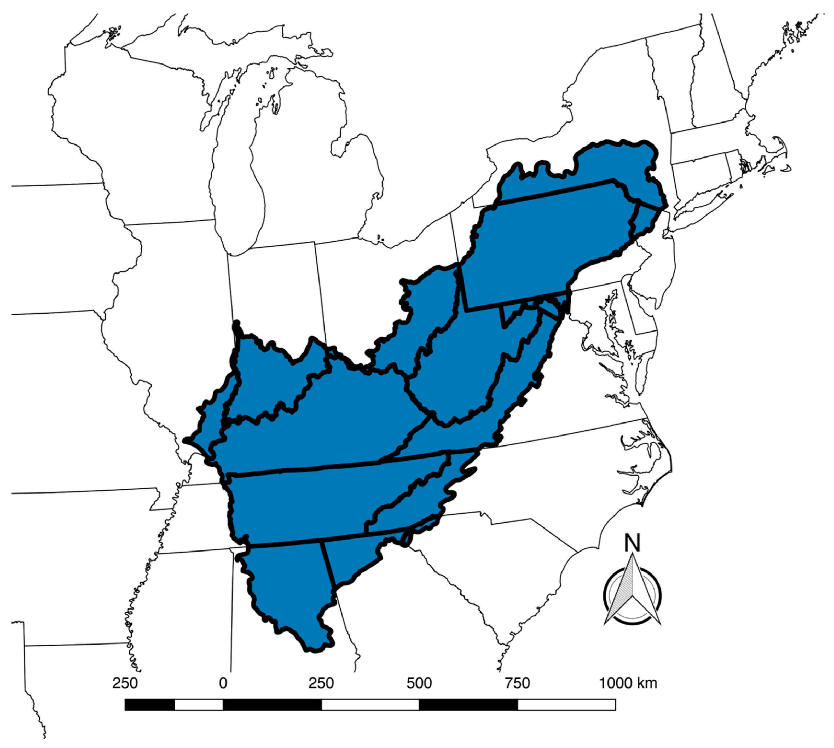
Our study focused on the rivers, streams, and landscape encompassed by the App LCC. The App LCC comprised 592,129 km
2, 266,307 HUC 12 watersheds, and intersects 15 states that range from central New York to the north, and central Georgia, Alabama, and Mississippi to the south [
20] (
Figure 1).
The eastern most extent reaches western New Jersey in the north and the western most portions of North and South Carolina, while reaching as far west as southern Illinois. The topography and habitat of the region are complex over such a large land area, which is comprised of six Level II ecoregions (U.S. EPA), 11 Freshwater Ecoregions, and seven major river basins and has been greatly influenced by the lack of glaciation and ancient geology, which gave rise to high levels of aquatic biodiversity. The App LCC region encompasses some of the most biologically diverse freshwater fish resources in the United States [
23]. This is particularly true in the southwestern portion of the region [
24]. As the 19th and 20th centuries have progressed, aquatic diversity has been impacted by anthropogenic activities that range from agricultural practices, land conversion, and extractive industries.
Through the aid of a steering committee comprised of 60 regional experts, which include academic scientists, state wildlife agency managers, non-governmental organization scientists, and conservation practitioners, we identified 52 predictor variables comprising six themes that are known to influence fish and aquatic macroinvertebrate communities (
Table A1). The themes included streamflow, geomorphic condition, connectivity, water quality, non-point source pollution, and point source pollution, and they were established and evaluated to understand large scale thematic processes that influence aquatic biota across the App LCC. The predictor data were compiled from regional and national datasets at the National Hydrography Dataset version 2 (NHD + V2) HUC12 watershed level (Final predictors used in BRT models are shown in
Table 1; a comprehensive list of predictor data with source is provided in
Appendix A).
Riparian corridors are known to be influential for developing ecological diversity [
25] and in structuring aquatic communities; hence, we used The Nature Conservancy’s Active River Area [
26] as a buffer into which land cover variables were clipped for modeling. The active river area framework provides an ecologically sound modelling mechanism to capture important variables that structure aquatic ecosystems [
26]. We centered and scaled all of the predictor variables to overcome instances where predictor variables had wide ranges resulting single predictors dominating models.
Our fish and aquatic macroinvertebrate community data were assembled from federal databases of national datasets (United States Environmental Protection Agency’s National Rivers and Streams Assessment and the National Fish Habitat Partnership). We used these community datasets as the predictors to assess the status of biological communities within HUC12 watersheds (
Table 2).
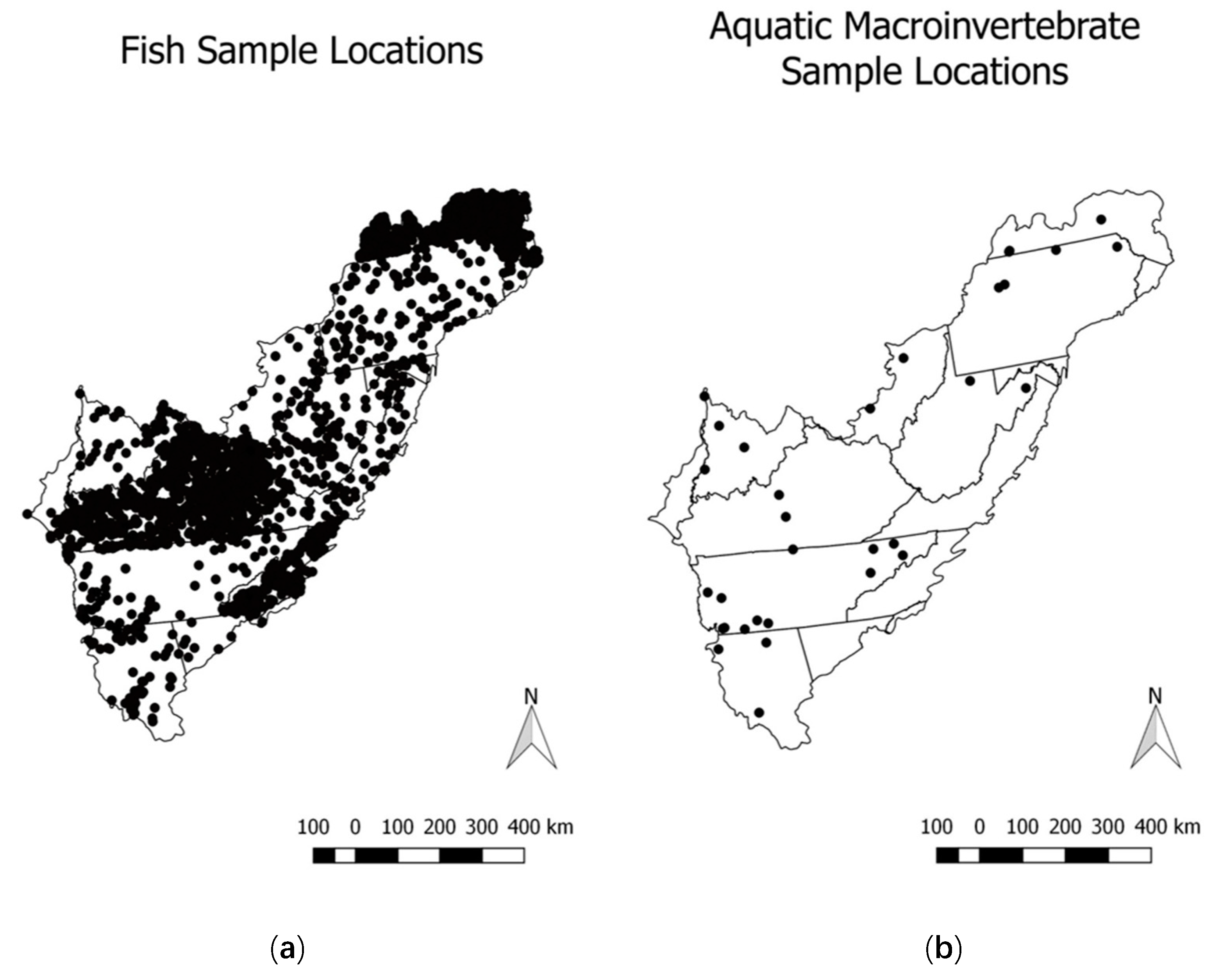
The sample point locations were spatially joined to HUC12 watersheds by projecting into a conic equal area projection in Quantum GIS [
27]. Our fish community dataset was comprised of 2991 sample sites across the region and was somewhat sparse (2991 locations within 266,309 HUC12 watersheds = 1.1%), but it exhibited good spatial distribution (
Figure 2).
Our aquatic macroinvertebrate dataset was comprised of only 194 sampling locations and it had poor spatial coverage (194 locations of 266,309 HUC12 watersheds = 0.07%) and distribution across the region (
Figure 2).
For fish, we calculated taxonomic richness and diversity and several functional group metrics while using the fish traits database that was provided by Frimpong and Angermeier [
28] and the tolerance database of Stoddard et al. [
29]. In total, we calculated 45 metrics for further analysis of fish responses to our predictor dataset; however, our final analysis used only nine of these metrics and these were further aggregated into three groupings that we called targets (e.g., Shannon diversity, functional group, fish taxa quality) (
Table 2). For aquatic macroinvertebrates the metrics modeled as response variables were % EPT (i.e., percent Ephemeroptera/Plecoptera/Trichoptera), % of total abundance comprised by the five most dominant taxa, % of total abundance that were tolerant taxa, and % of the total abundance that were intolerant taxa (
Table 2). These four metrics were aggregated into a target called macroinvertebrate taxa quality (
Table 2).
Prior to model development, we successively screened all of the predictor variables (e.g., [
3,
11]). Screening included evaluating predictor variables for: 1) range, where predictor variables with small range (e.g., <4) were removed, 2) percent zero or NAs, where variables with >33% zero or NA were removed, and 3) percent values equal to the mode, where the variables with >75% of the values were the same were removed. After screening, the 52 predictor variables were reduced to 24, which comprised six themes (
Table 1). Subsequently, we employed boosted regression trees (BRTs) to predict fish and aquatic macroinvertebrate response variables at the watershed scale (
Table 2). Boosted regression trees are robust to missing data, have both explanatory and predictive power, and they are capable of handling complex relationships that are both non-linear and interactive without the need for prior data transformation. By iteratively fitting and combining simple regression models, BRT models improve model structure and predictive performance. Tree complexity and learning rate were systematically altered to identify the optimal model structure. We reduced model complexity by removing the redundant variables (r > 0.80) and variables with minimum variation among sites. Global models were developed with the remaining variables and then further simplified while using scree plots of the predictor relative influence. Simplified models were retained if their cross-validation was greater than or equal to that of the global model. BRT models were developed with methods and code that were provided by Elith et al. [
16] while using Program R: A language and environment for statistical computing [
30]. Initial analyses were performed across the entire geography without accounting for regional differences (i.e., ecoregions), but we used Freshwater Ecoregions of the World [
31] to understand these regional differences due to a clear need for the inclusion of regional differences within the models. Freshwater ecoregions attempt to place aquatic ecosystems in a biogeographical framework that is based on ecological and evolutionary patterns of fish distributions [
31]. We aggregated the 11 ecoregions that comprised the App LCC into four due to low sample site numbers in some Freshwater Ecoregions. The four aggregated ecoregions and their composite Freshwater Ecoregions were Atlantic Slope (Appalachian Piedmont, Chesapeake Bay, Northeast US and Southeast Canada Atlantic Drainages), Cumberland (Cumberland River Basin), Ohio (Teays-Ohio and Laurential Great Lakes River Basins), and Tennessee (Tennessee and Mobile Bay River Basins). The regional models were successfully run for fish, but we were unable to model aquatic macroinvertebrates regionally due to the lack of spatial coverage, and we therefore retained models for the entire geography for aquatic macroinvertebrates.
Predictions of response variables from BRT models were centered and scaled. As a multimetric approach, the predicted responses (biological metrics in
Table 1) were then averaged within their target group (see
Table 1) and further condensed via averaging into overall fish and aquatic macroinvertebrate scores. Boosted regression trees provide the relative influence of predictor variables in the modelling of responses, and we averaged these relative influences within our thematic framework (see above and
Table 1) for each fish and aquatic macroinvertebrate response variable.
3. Results
The screening process reduced the total number of predictor variables to 37 from 52. When the predictor variables were correlated, we attempted to retain the variable that was most responsive to our models; however, this was not formally tested. The themes with the greatest number of predictor variables were non-point source pollution and point source pollution (each with eight variables). While the theme with the least number of predictor variables was geomorphic condition (two variables) (
Table 1).
Below, we present the results from the boosted regression tree models where the models were run with all ecoregions together for both fish and aquatic macroinvertebrates. We refer to this as a “Global” model (see below). After which, we present the results where separate models were run for each Freshwater Ecoregion (defined in the materials and methods section). We refer to these models as regional models and, because there were not enough data points within the regional data sets for aquatic macroinvertebrates, they were developed for fish only.
3.1. Global Models
Boosted regression tree models were developed for 45% (28/62) of the response variables; however, we only retained 12 (eight and four response variables for fish and aquatic macroinvertebrates, respectively) for our final multimetric index of biotic condition (
Table 2). Response variables were collapsed into targets, where, for the fish category, we retained three targets (Shannon diversity, functional group, and taxa quality) and for aquatic macroinvertebrates, we retained macroinvertebrate taxa quality as the only target.
The range of variance that was explained by the BRT models was 48% for percentage of invertivore taxa to 85% for fish taxa diversity (
= 73%) for fish and 76% for percentage of the five dominant taxa to 89% for percentage of tolerant taxa (
= 81%) for aquatic macroinvertebrates. For the fish BRT models, the cross-validated deviance ranged from 32% for percentage of invertivore taxa to 69% for fish taxa diversity (
= 52%), while it ranged from 24% for percentage of the five dominant taxa to 76% for percentage of tolerant taxa for aquatic macroinvertebrates (
= 41%) (
Table 3).
The lower cross validated deviances for aquatic macroinvertebrates relative to those of fish are likely due to the lack of spatial data coverage in the aquatic macroinvertebrate data (
Figure 2b).
The predictor variables that had the greatest relative influence were freshwater ecoregion and network percent impervious surface for fish and aquatic macroinvertebrates based on the results of the BRT models, respectively. Those with the least relative influence were how confined a stream reach was (CONF_CL) and watershed mine density for fish and aquatic macroinvertebrates, respectively (
Table 4).
The theme with the greatest cumulative relative influence for fish was geomorphic condition (46.6%) and for aquatic macroinvertebrates was water quality (41.7%), while point source pollution was the least important theme for both fish (1.4%) and aquatic macroinvertebrates (0.8%). The relative thematic influence was variable between response variables; where, for example, the flow theme was the most influential for % EPT (27.4%), but the most influential theme was water quality for % intolerant taxa (87.9%) (
Table 5).
3.2. Regional Models
Regional differences were evident in the results of the relative influence of predictor variables on responses. For example, the variable with the greatest relative influence for richness in the Atlantic Slope data was July temperature (22.8%), for the Cumberland River Basin, was ground flow recharge (17.6%), for the Ohio River Basin, was average catchment elevation (21.4%), and for the Tennessee River Basin, it was dam storage capacity (8.2) (
Table 6).
Additionally, the relative influence varied widely within a given region for the same predictor variable, but for different response variables. For example, k-factor (a measure of soil erodibility) had the 24th most influence on diversity in the Atlantic Slope, but it was the fourth most influential variable in the % herbivore taxa model. The standard deviation that was associated with the relative influence of predictor variables for a specific region was also variable; where, for example, for invertivore diversity the standard deviation was 2.4, 2.6, 5.1, and 4.3 for the Atlantic Slope, the Cumberland River Basin, the Ohio River Basin, and the Tennessee River Basin, respectively.
The mean relative influence for themes were also somewhat variable across regions; where, for example, flow was the most influential theme for each region for the BRT model for the % of species that prefer coarse sediment. However, for the % of tolerant fish species, the flow theme represented the fourth most influential theme for the Atlantic Slope (
= 1.7%), third most for the Cumberland River Basin (
= 2.5%), second most for the Ohio River Basin (
= 2.7%), and first most for the Tennessee River Basin (
= 3.6%) (
Table 7).
Generally, geomorphic condition was the most influential theme followed by flow, non-point source pollution, water quality, connectivity, and point source pollution when averaged across all of the response variables. With little variation, the themes were consistent in terms of their relative influence across regions; for example, non-point source pollution was the fourth most influential theme for the Atlantic Slope, the Ohio River Basin, and the Tennessee River Basin, but the fifth most influential for the Cumberland River Basin.
3.3. Fish Models
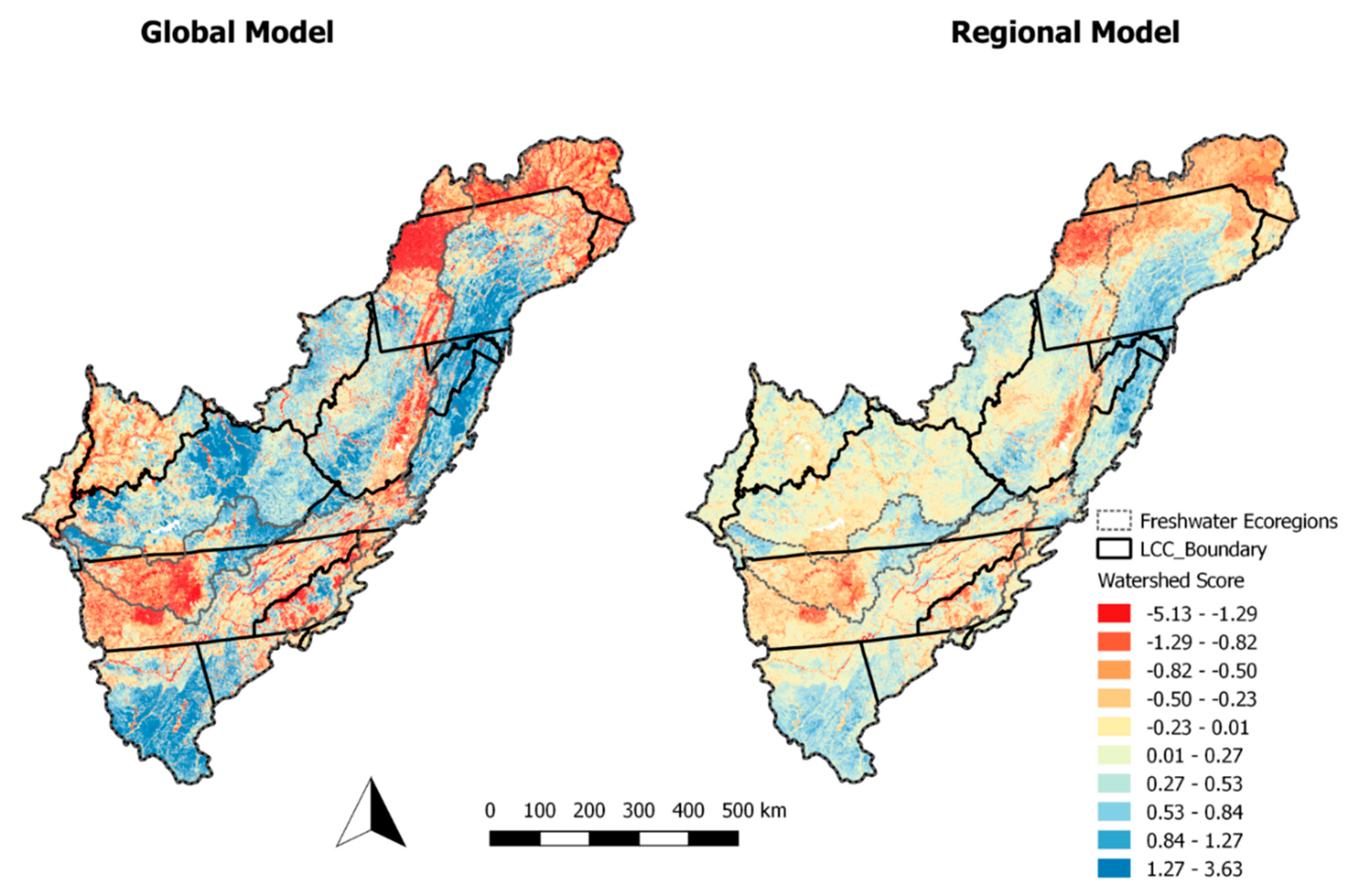
The model results suggest there are distinct areas of the App LCC region that exhibit characteristics of poor biological condition (i.e., watershed score) (
Figure 3).
For example, western Tennessee (i.e., the Southeastern Plains) and the northern-most portion of the region (i.e., the Atlantic Highlands). Additionally, large rivers tended to exhibit poor biological condition. This was especially true in areas with high agricultural land use (i.e., east Tennessee). Regions where the models displayed relatively good biological condition were largely in areas free from agricultural land use. However, large rivers exhibited poor biological condition, even in areas with good biological condition.
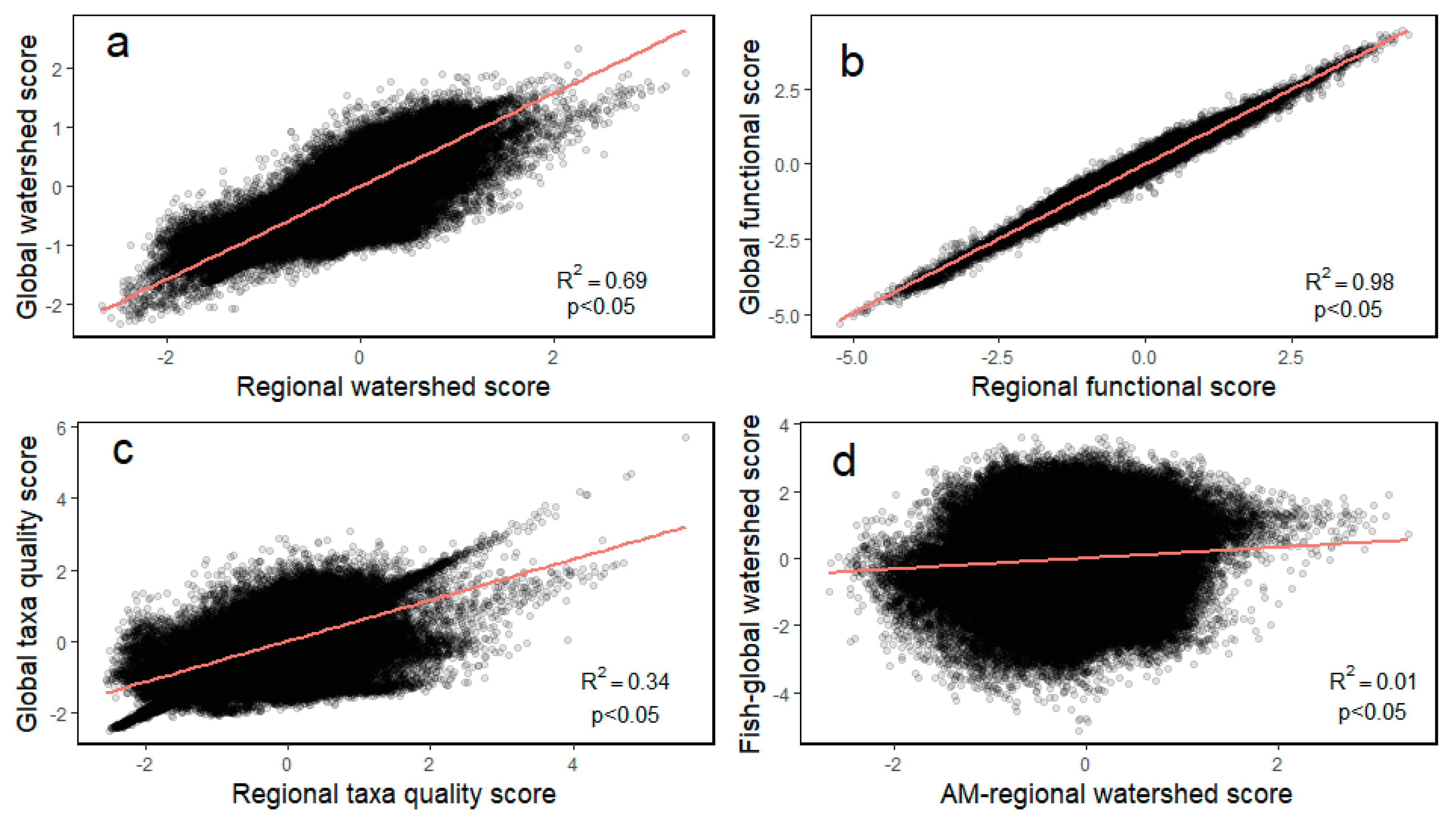
Pearson correlations between the global and regional models were variable and ranged from 0.33 (% intolerant taxa) to 0.99 (% invertivore taxa) for pairwise comparisons. The overall indices for watershed scores (i.e., biological condition) were moderately correlated (0.69). The targets were highly correlated for the functional group (0.98) but, were relatively poorly correlated for taxa quality (0.34) (
Table 8) (
Figure 4).
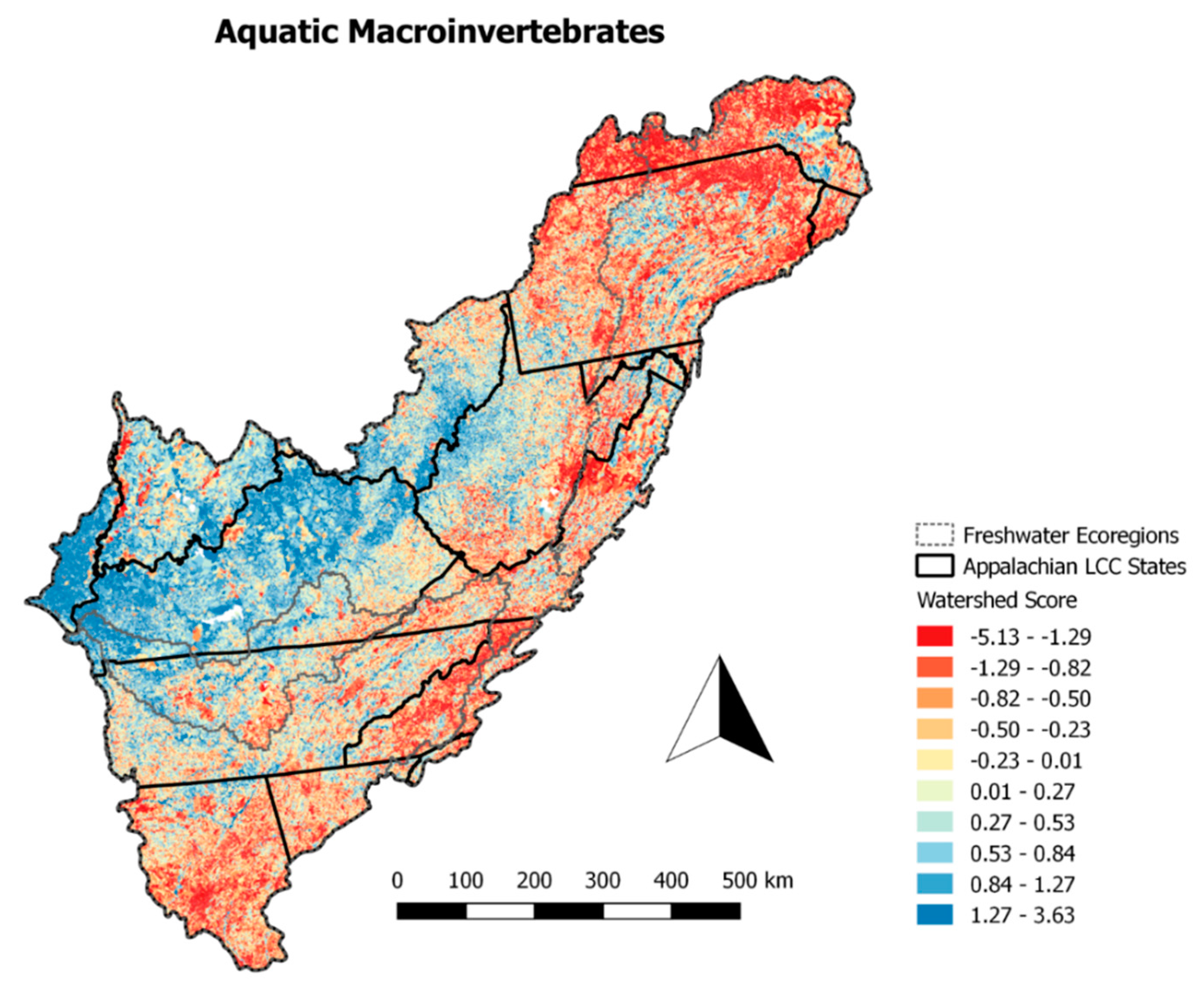
3.4. Aquatic Macroinvertebrate Model
We were unable to develop regional models for aquatic macroinvertebrates due to the data set being sparse in some regions. The global model for aquatic macroinvertebrates showed poor ability to identify areas with a good and bad biological condition. Only very large geographic regions were distinguishable from one another. For example, the western portion of the App LCC region was identified as having relatively higher biological condition when compared to the eastern and northern portions of the region. Where the fish models identified large rivers as having poor biological condition, the aquatic macroinvertebrate models were unable to identify the biological condition at this scale (
Figure 5).
Additionally, the Pearson correlation coefficient between the aquatic macroinvertebrate watershed score and those of the global (
Figure 4) and regional fish watershed scores was 0.01 for both.
4. Discussion
Freshwater ecosystems are highly threatened worldwide. In North America, the Appalachian LCC region is a particularly valuable aquatic ecosystem due, in large part, to its high aquatic biodiversity. It is also a region of great conservation concern due to current and projected rapid land cover change (i.e., urbanization), biodiversity loss, habitat fragmentation, and climate change [
17,
20]. Models, such as the ones presented here, and others (e.g., [
3,
5]), which provide insight into how land use affects aquatic resources (e.g., fish and aquatic macroinvertebrates), are valuable tools for identifying areas of greatest concern for restoration activities and those areas in greatest need of increased and/or continued protection [
32,
33].
Multimetric indices may be beneficial in identifying a biological condition across large geographies. Our results suggest that multimetric scores (i.e., watershed scores) corroborate one another at the global and regional scales (see
Table 8), which indicate that the predictor variables we used were responsive in a consistent manner across scales. This is an important finding, as the ability to rely on a consistent set of landscape variables enables cross-regional and cross-scale comparisons, which can be particularly important when data sets are assembled from multiple sources [
3].
The individual predictors that most commonly had high relative influence for fish metrics (i.e., was ranked in the top ten percent of predictors within an individual metric) were primarily related to geomorphic condition (e.g., erosive and resistive forces) and flow regime (e.g., storage and recharge capacity). However, those with the highest relative influence for aquatic macroinvertebrates were primarily related to sources of pollution (e.g., road crossings, nitrogen, and silt). Our results reinforce those of Hill et al. [
5], who found that agriculture and urbanization were the primary drivers of landscape impacts on aquatic macroinvertebrates. The differences in driving factors for fish and aquatic macroinvertebrates suggest that, at a large spatial scale, such as that presented here, the important land use factors that influence aquatic communities may differ somewhat and mitigation efforts to overcome these large-scale stressors likely need to have some taxonomic specificity.
The relative influence of individual predictors to our boosted regression tree models was variable between regions in our regional models. This indicates the high variability between regions regarding what environmental factors influence community structure. These findings are not surprising, as they are congruent with other large-scale biological condition assessments [
3,
5] and have been found to be a shortcoming of MMIs [
34,
35]. While individual predictors were relatively variable between regions, our models suggested themes (i.e., combined predictors) were more consistent; yet, some discrepancies between regions still existed. We chose to condense predictor variables into themes as a higher order mode of understanding of how these groups of stressors impacted fish and aquatic macroinvertebrates. The themes that exhibited the greatest influence on fish watershed scores across the entire region were geomorphic condition and flow regime. The geomorphic condition in our analysis was a measure of soil stability and erosivity. This finding is unsurprising, as aquatic taxa are known to be sensitive to sedimentation. Surprisingly, point source pollution and connectivity were the least influential. This is likely due to these two factors being measured somewhat sparsely (i.e., few watersheds have NPDES sites) on the landscape and not necessarily in close proximity to biological samples. For example, NPDES density, which is a measure of point source pollution, is likely to exhibit strong influence on aquatic biota in the immediate area, but these sites are scattered across the landscape and, thus, across a large region, such as the App LCC region, they were less influential in our models than predictors that have greater spatial representation (e.g., soil erosivity).
A high correlation between the global and regional fish multimetric indices suggests that the predictor variables used were responsive across both scales. While there was high correlation between global and regional fish multimetric indices (i.e., watershed score), there was very low correlation between multimetric indices from either of the fish models and the global aquatic macroinvertebrate model. The low correlation between the fish watershed scores and aquatic macroinvertebrate watershed scores is most likely due to the low number of sites (N = 334), which results in poor spatial coverage for our aquatic macroinvertebrate data set, as compared to the good spatial distribution and relatively high number of sites (N = 8355) in our fish data set. Correlations between the fish and aquatic macroinvertebrate indices are likely to be higher when the same, or nearby, sites are sampled for both. For example, at 18 sites in the River Raisin watershed in Michigan, correlations between fish and aquatic macroinvertebrate indices ranged from 0.21 to 0.51 [
36]. Additionally, stressors have been found to affect fish and aquatic macroinvertebrates similarly. Free flowing stream sections of the Fox River, IL exhibited higher index scores for both fish and aquatic macroinvertebrates when compared to sections of the river above low-head dams [
37].
Esselman et al. [
3] suggested regional stratification for analyses that span large geographies, while also including multiple biological response variables, and using statistical modeling techniques that are non-linear would lead to improved multimetric indices. This is precisely the approach that we took modeling biological condition across the 15 state App LCC region. However, one major difference between our study and previous studies is that previous work to develop multimetric indices across broad geographies included regional influences by using Omernick ecoregions [
3,
5,
15] (Whittier et al., 2007; Esselman et al. 2013; and, Hill et al. 2017). Omernick ecoregions are a spatial framework that includes aquatic and terrestrial ecosystems [
38]; however, we used Freshwater Ecoregions of the World for our analysis, because they were developed on a framework that focused exclusively on aquatic ecosystems with fish as the focal taxonomic group [
31].
Another difference between our work and previous work is that we aggregated both predictor and response variables into themes and targets respectively. By aggregating predictor variables into themes, we were able to identify categories of predictors that were influential in structuring fish and aquatic macroinvertebrate communities in aggregate (e.g., watershed score for fish), as well as for individual response variables (e.g., % EPT). Response variable aggregation allows for a greater understanding of how individual and aggregate predictors (i.e., themes) structure fish and/or aquatic macroinvertebrate communities in a more functional manner. For example, two targets (e.g., fish functional group and fish taxa quality) may respond differently to the same stressor. Understanding which higher order stressors (theme) affect our targets (fish functional group) might lend insight into more effective regional management and conservation strategies. Our results suggest that regional variability of the relative influence of predictor variables should garner significant consideration as the stressors that affect fish and aquatic macroinvertebrates were not the same from ecoregion to ecoregion. Furthermore, care should be taken when using large scale modeling efforts such as ours to make management recommendations across large geographies that span more than one ecoregion, as thematic importance was variable between regions.
While we were able to develop regional models for fish indices, unfortunately, we were unable to develop regional aquatic macroinvertebrate models due to low numbers of sample sites. As aquatic macroinvertebrates are known to be good indicators of biological condition [
39,
40,
41], we believe that there needs to be increased systematic sampling efforts that result in an increased number of sites that are spatially dispersed across multiple freshwater ecoregions and that include known areas of both high and low biological integrity. In doing so, models such as the one provided here (see also Hill et al. 2017 and Esselman et al. 2013 [
3,
5] can be improved in their ability to provide managers with information to help guide local plans within a regional context. For example, mitigation efforts that aim to provide ecological lift to a watershed might look for areas that have been identified as having poor condition but surrounded by watersheds with good condition or, alternatively, these models could be used to identify good quality watersheds that are in need of protection from multiple encroaching stressors.
5. Conclusions
We combined and used multiple biotic and abiotic datasets to model stream condition across the Appalachian LCCs 15 state boundary (i.e., central and southern Appalachians). We developed separate fish and aquatic macroinvertebrate steam condition models highlighting the existence of both similarities and differences in how environmental factors structure these two aquatic taxonomic communities while using BRTs. Overall, correlation existed between fish and aquatic macroinvertebrate models and global and regional fish models. Furthermore, there was high correlation between global and regional fish models for most of the fish metrics evaluated. We were unable to create aquatic macroinvertebrates regional models due to low sample size regionally; however, for fish, separate models for each of the Freshwater Ecoregions varied in what environmental factors were most important in structuring aquatic communities, which exemplified the need to carefully consider ecoregional factors when developing cross-ecoregion spatial plans and management suggestions. Biological samples are difficult and expensive to collect, and effort varies between taxa, and this results in uneven distributions in both the number of samples and spatial distribution between taxa making it difficult to create MMIs that can better represent the condition of aquatic resources across broad geographies. Careful selection of biological sample locations that are representative of the spectrum spanning from high quality to low quality environmental conditions that are spatially well dispersed can greatly enhance the ability of models such as ours to inform spatial and management plans. Additionally, common sample locations for various taxa would be useful to improve the comparison of environmental responses among and between taxa.
We recommend a centralized database where these records are made available for public download, where efforts such as ours can be more easily replicated, improved upon, and then performed at various spatial scales. With an extensive and systematic sampling approach that includes both fish and aquatic macroinvertebrates and it is integrated across jurisdictional boundaries the ability to develop accurate models of large geographies will improve. Such improved spatial models will lend greater confidence in such indices, which will only increase the ability of managers, conservation practitioners, and scientists alike to address and meet regional conservation goals.


