Monitoring Effects of Land Cover Change on Biophysical Drivers in Rangelands Using Albedo


Abstract
:1. Introduction
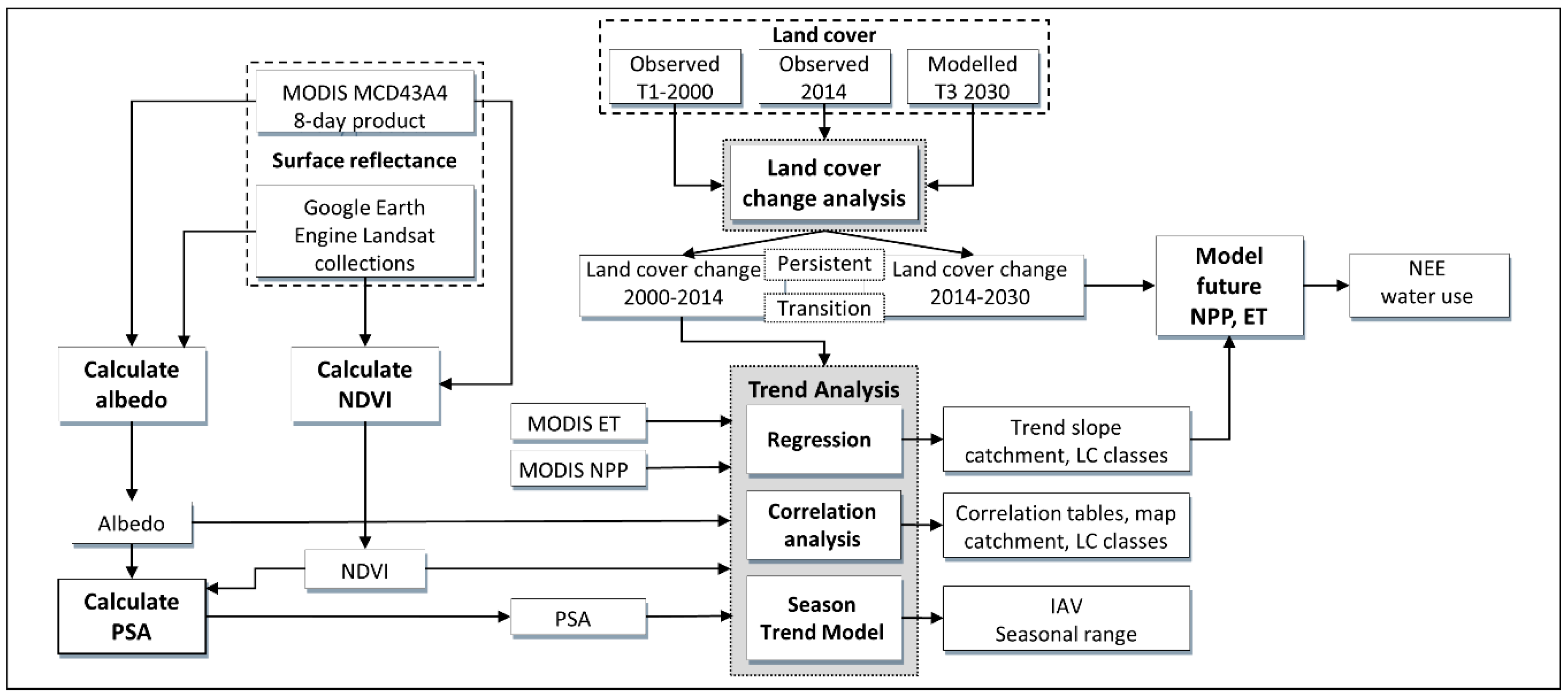
2. Materials and Methods
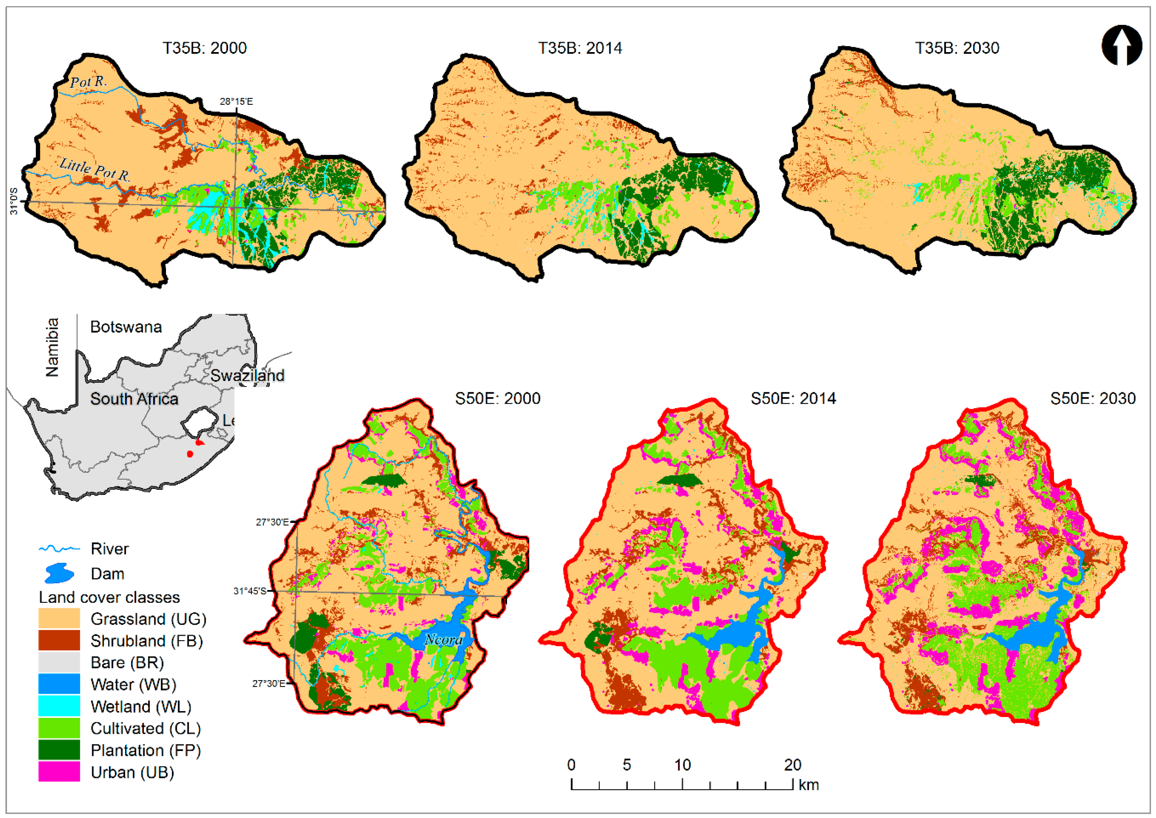
2.1. Land Cover Change
2.2. Satellite Data
2.2.1. Albedo
2.2.2. Normalised Difference Vegetation Index (NDVI) and Peak Season Albedo
2.2.3. Moderate Resolution Imaging Spectroradiometer (MODIS) Net Primary Production (NPP) and Evapotranspiration (ET)
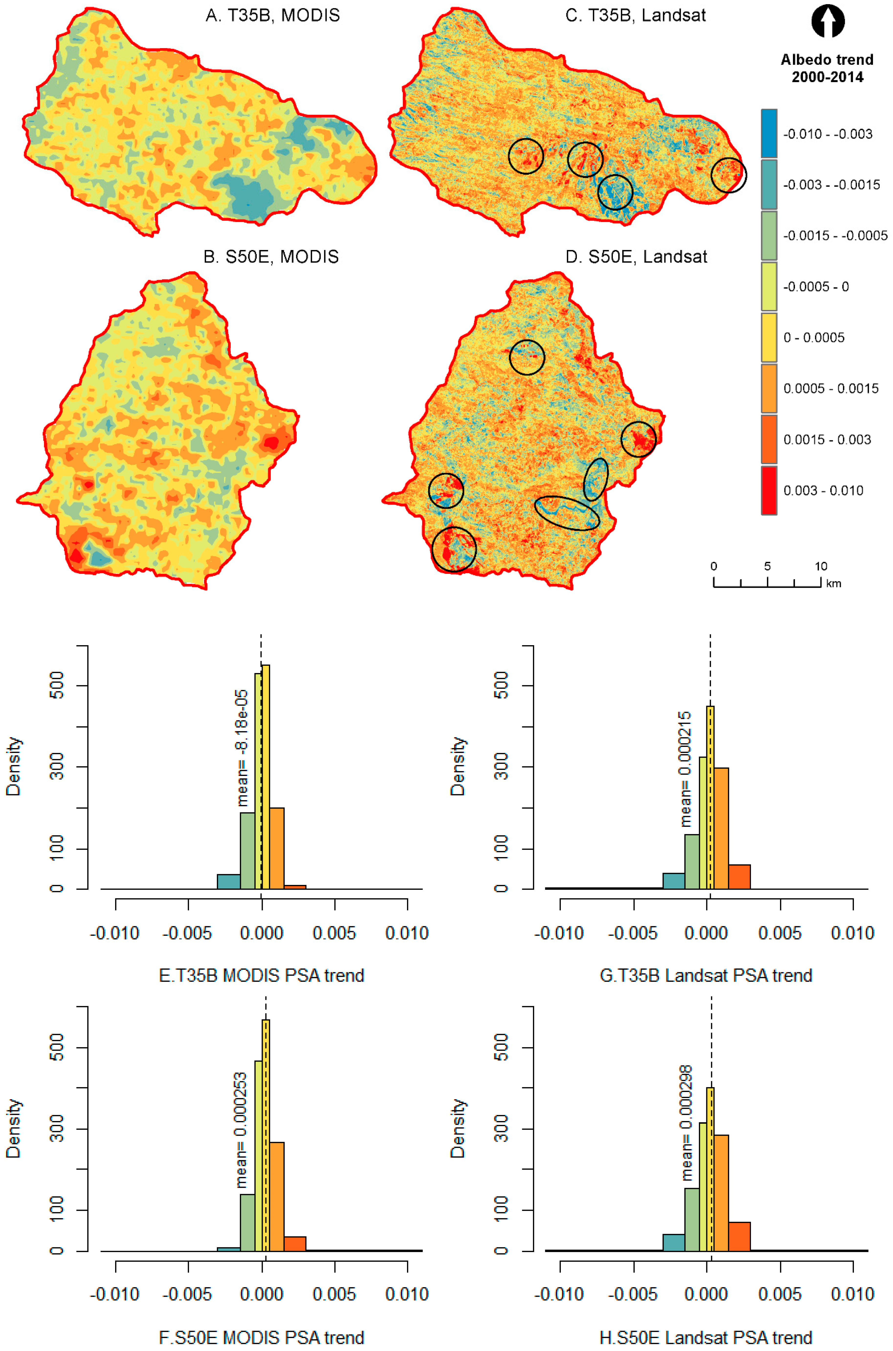
2.3. Trend Analysis
3. Results
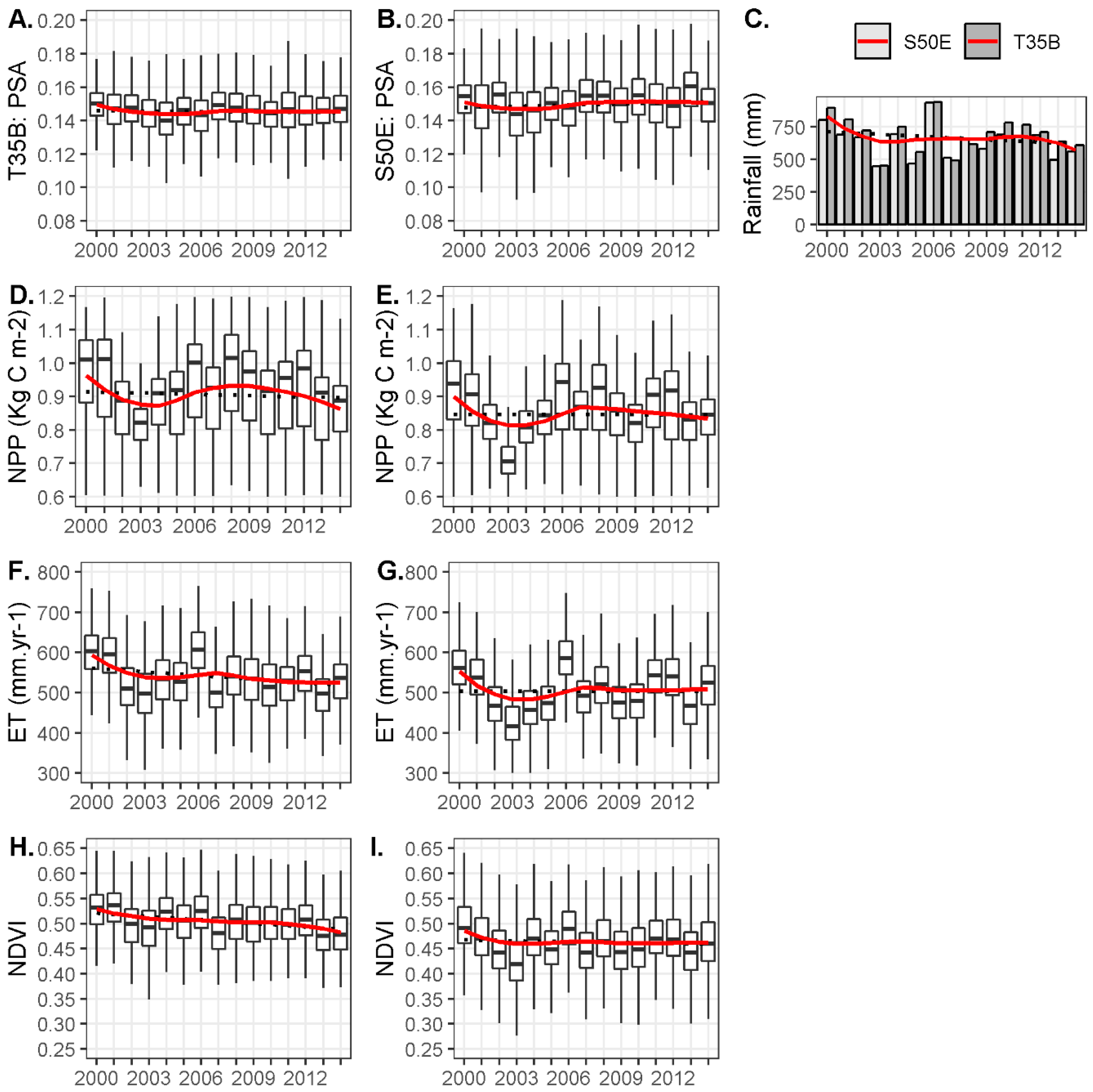
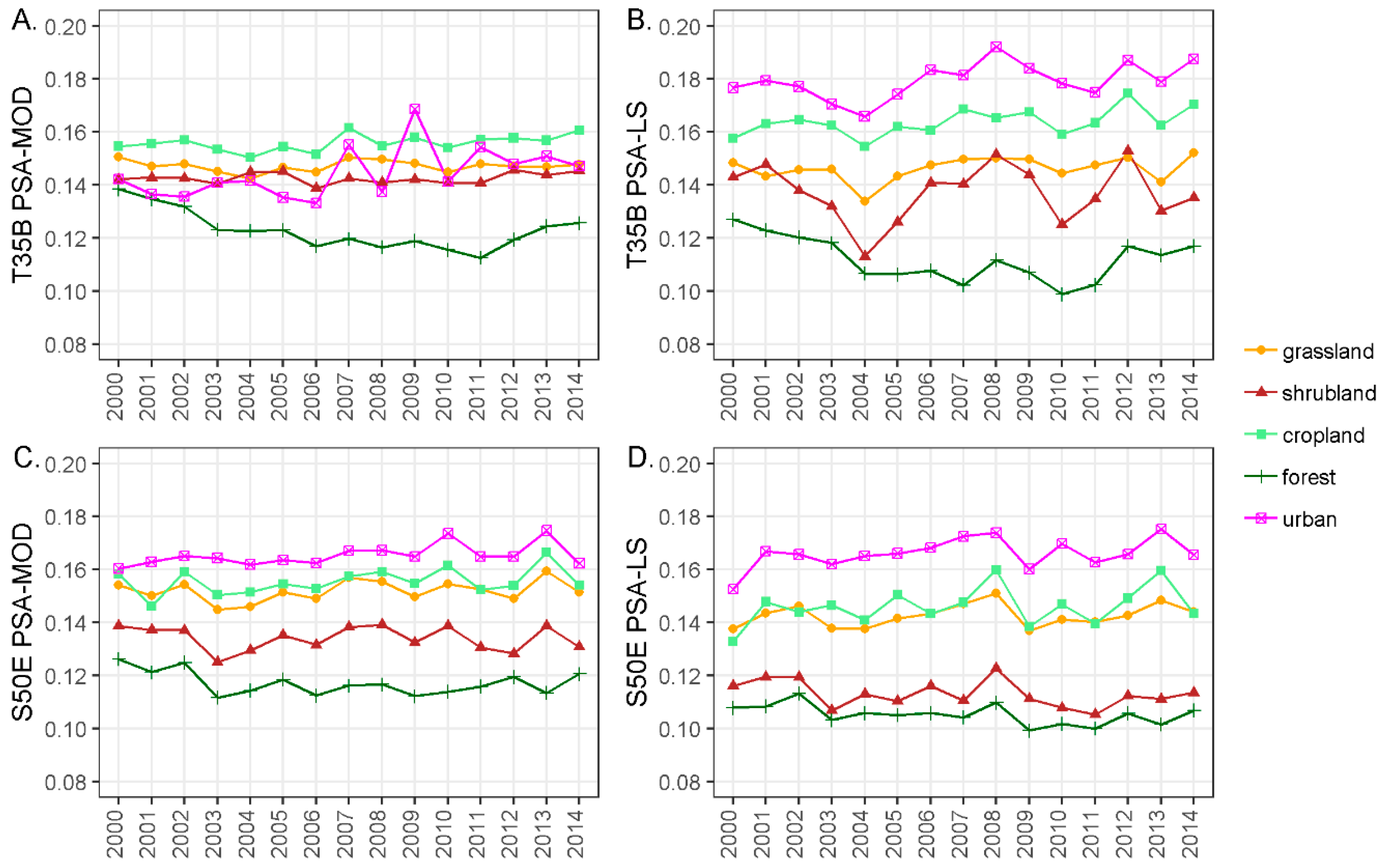
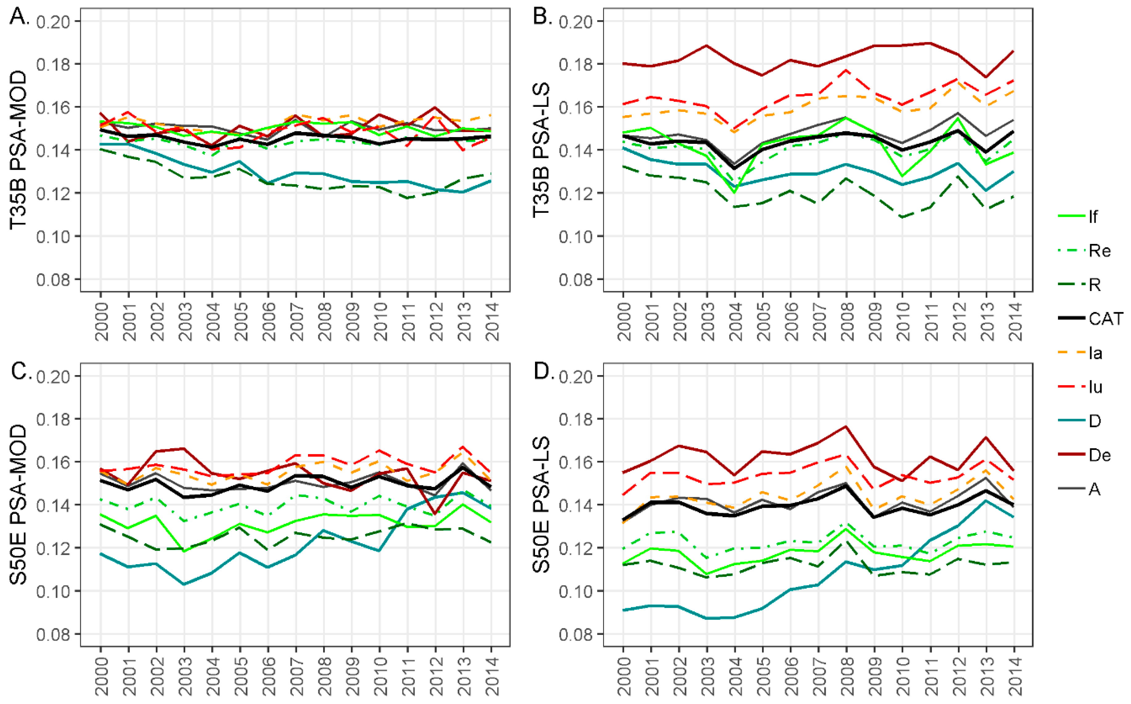
3.1. Catchment Level Peak Season Albedo (pSA), NPP, ET and NDVI
3.2. Land Cover Trajectories
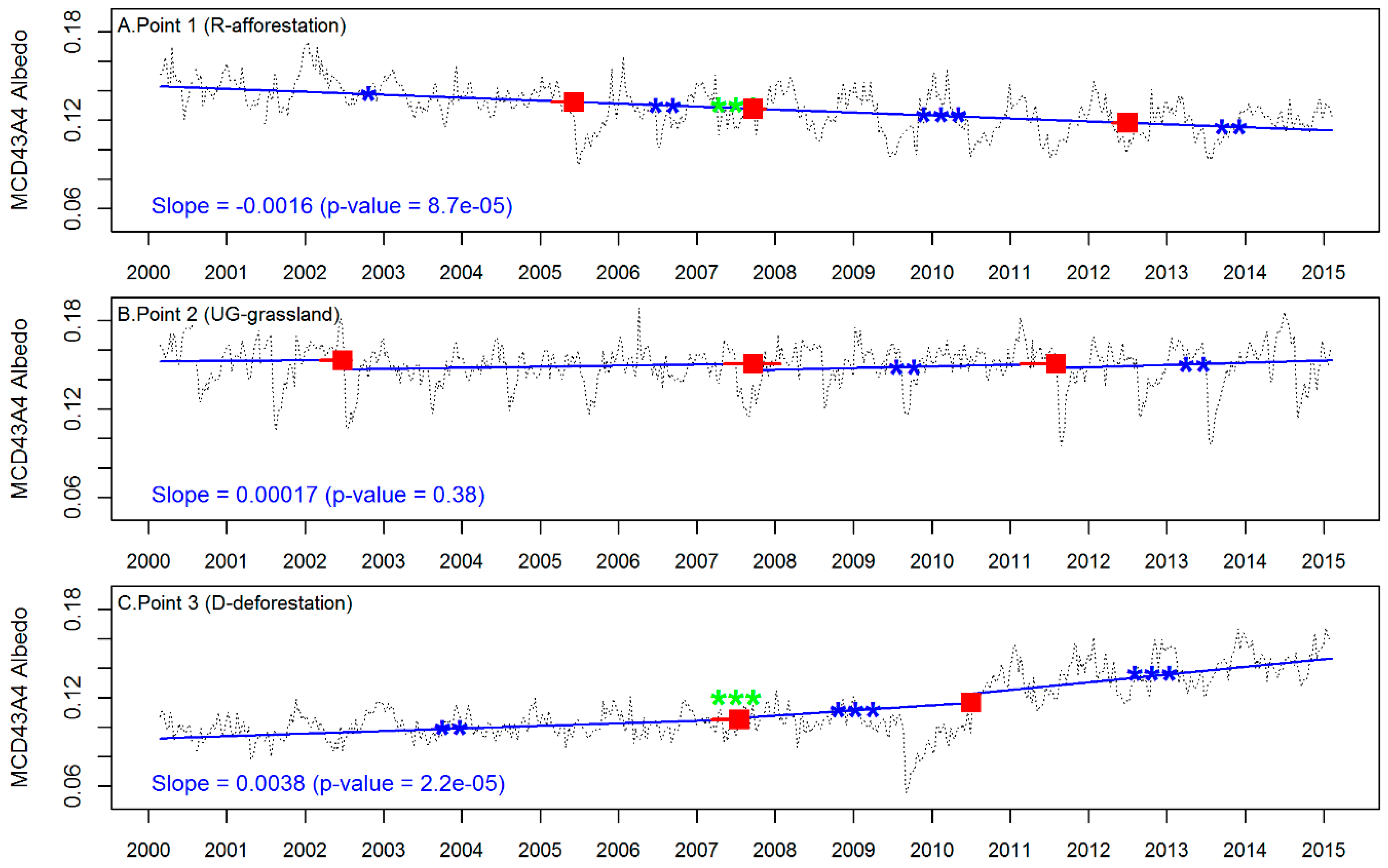
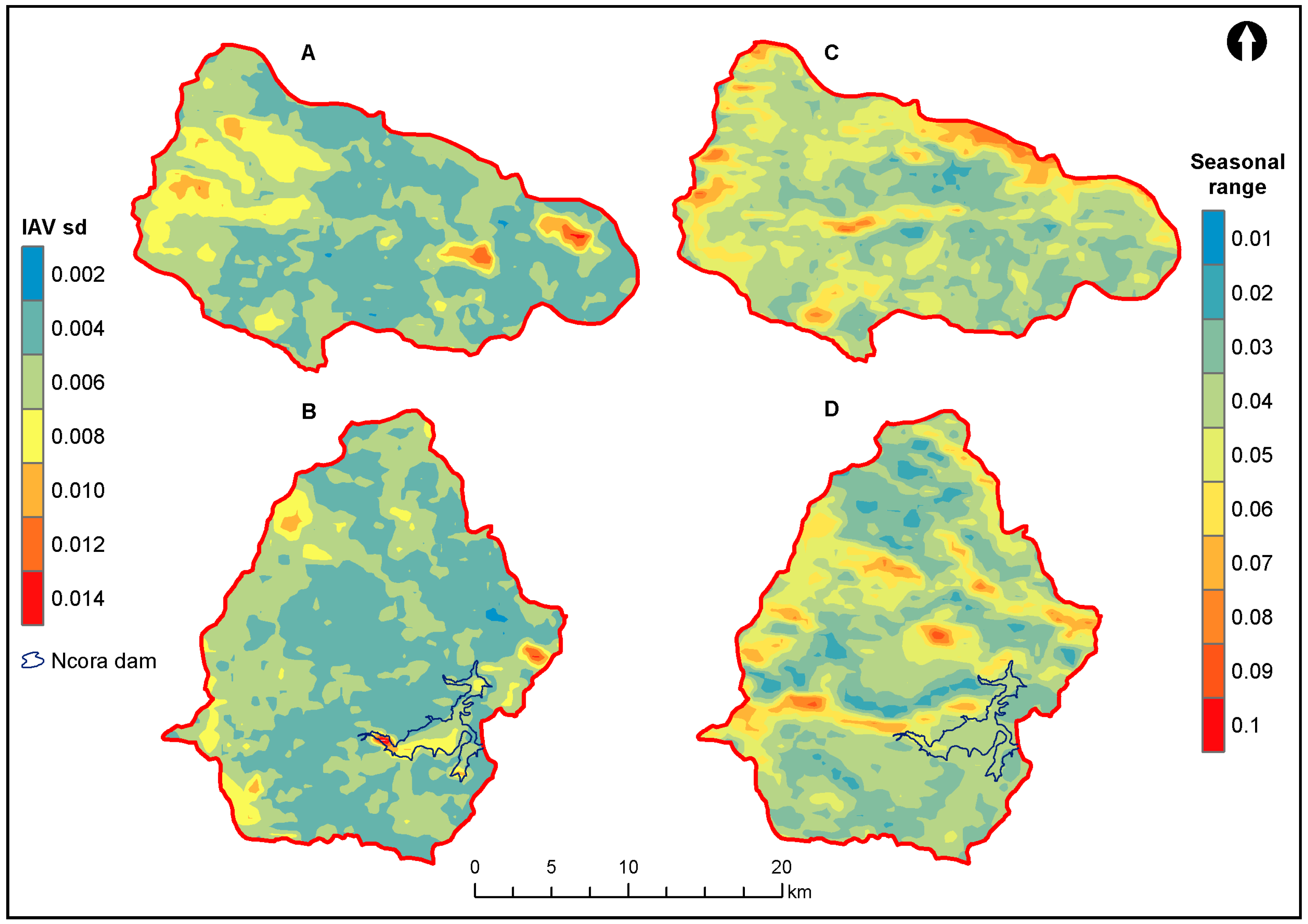
3.3. Season-Trend Model
3.4. Modelling ET and NPP
4. Discussion
4.1. Land Cover Change and Trend Analysis
4.2. Catchment Differences
4.3. Implications
5. Conclusions
Supplementary Materials
Author Contributions
Funding
Acknowledgments
Conflicts of Interest
References
- Betts, R.A. Biogeophysical impacts of land use on present-day climate: Near-surface temperature change and radiative forcing. Atmos. Sci. Lett. 2001, 2, 1–8. [Google Scholar] [CrossRef]
- Gwate, O.; Mantel, S.K.; Gibson, L.A.; Munch, Z.; Palmer, A.R. Exploring dynamics of evapotranspiration in selected land cover classes in a sub-humid grassland: A case study in quaternary catchment S50E, South Africa. J. Arid Environ. 2018, 157, 66–76. [Google Scholar] [CrossRef]
- Forkel, M.; Carvalhais, N.; Verbesselt, J.; Mahecha, M.D.; Neigh, C.S.R.; Reichstein, M. Trend Change detection in NDVI time series: Effects of inter-annual variability and methodology. Remote Sens. 2013, 5, 2113–2144. [Google Scholar] [CrossRef]
- Münch, Z.; Okoye, P.I.; Gibson, L.; Mantel, S.; Palmer, A. Characterizing Degradation Gradients through Land Cover Change Analysis in Rural Eastern Cape, South Africa. Geosciences 2017, 7, 7. [Google Scholar] [CrossRef]
- Palmer, A.R.; Finca, A.; Mantel, S.K.; Gwate, O.; Münch, Z.; Gibson, L.A. Determining fPAR and leaf area index of several land cover classes in the Pot River and Tsitsa River catchments of the Eastern Cape, South Africa. Afr. J. Range Forage Sci. 2017, 34, 33–37. [Google Scholar] [CrossRef]
- Lei, T.; Pang, Z.; Wang, X.; Li, L.; Fu, J.; Kan, G.; Zhang, X.; Ding, L.; Li, J.; Huang, S.; et al. Drought and Carbon Cycling of Grassland Ecosystems under Global Change: A Review. Water 2016, 8, 460. [Google Scholar] [CrossRef]
- Bright, R.M.; Cherubini, F.; Strømman, A.H. Climate impacts of bioenergy: Inclusion of carbon cycle and albedo dynamics in life cycle impact assessment. Environ. Impact Assess. Rev. 2012, 37, 2–11. [Google Scholar] [CrossRef]
- Lutz, D.A.; Howarth, R.B. Valuing albedo as an ecosystem service: Implications for forest management. Clim. Chang. 2014, 124, 53–63. [Google Scholar] [CrossRef]
- Bonan, G.B. Forests and climate change: forcings, feedbacks, and the climate benefits of forests. Science 2008, 320, 1444–1449. [Google Scholar] [CrossRef]
- Georgescu, M.; Lobell, D.B.; Field, C.B. Direct climate effects of perennial bioenergy crops in the United States. Proc. Natl. Acad. Sci. USA 2011, 108, 4307–4312. [Google Scholar] [CrossRef]
- Swann, A.L.S.; Fung, I.Y.; Chiang, J.C.H. Mid-latitude afforestation shifts general circulation and tropical precipitation. Proc. Natl. Acad. Sci. USA 2012, 109, 712–716. [Google Scholar] [CrossRef] [PubMed]
- Davin, E.L.; de Noblet-Ducoudré, N.; Davin, E.L.; Noblet-Ducoudré, N. de Climatic Impact of Global-Scale Deforestation: Radiative versus Nonradiative Processes. J. Clim. 2010, 23, 97–112. [Google Scholar] [CrossRef]
- Oelofse, M.; Birch-Thomsen, T.; Magid, J.; de Neergaard, A.; van Deventer, R.; Bruun, S.; Hill, T. The impact of black wattle encroachment of indigenous grasslands on soil carbon, Eastern Cape, South Africa. Biol. Invasions 2016, 18, 445–456. [Google Scholar] [CrossRef]
- O’Connor, T.G.; Puttick, J.R.; Hoffman, M.T. Bush encroachment in southern Africa: Changes and causes. Afr. J. Range Forage Sci. 2014, 31, 67–88. [Google Scholar] [CrossRef]
- Gouws, A.J.; Shackleton, C.M. Abundance and correlates of the Acacia dealbata invasion in the northern Eastern Cape, South Africa. For. Ecol. Manag. 2019, 432, 455–466. [Google Scholar] [CrossRef]
- Rotenberg, E.; Yakir, D. Contribution of Semi-Arid Forests to the Climate System. Science 2010, 327, 451–455. [Google Scholar] [CrossRef]
- Cunha, J.E.B.L.; Nóbrega, R.L.B.; Rufino, I.A.A.; Erasmi, S.; Galvão, C.; Valente, F. Surface albedo as a proxy for land-cover change in seasonal dry forests: Evidence from the Brazilian Caatinga biome. EarthArXiv. 2018. Available online: https://eartharxiv.org/zjd58/ (accessed on 30 January 2019). [CrossRef]
- Wang, Z.; Schaaf, C.B.; Sun, Q.; Kim, J.; Erb, A.M.; Gao, F.; Román, M.O.; Yang, Y.; Petroy, S.; Taylor, J.R.; et al. Monitoring land surface albedo and vegetation dynamics using high spatial and temporal resolution synthetic time series from Landsat and the MODIS BRDF/NBAR/albedo product. Int. J. Appl. Earth Obs. Geoinf. 2017, 59, 104–117. [Google Scholar] [CrossRef]
- Cai, H.; Wang, J.; Feng, Y.; Wang, M.; Qin, Z.; Dunn, J.B. Consideration of land use change-induced surface albedo effects in life-cycle analysis of biofuels. Energy Environ. Sci. 2016, 9, 2855–2867. [Google Scholar] [CrossRef]
- Gibson, L.; Münch, Z.; Palmer, A.; Mantel, S. Future land cover change scenarios in South African grasslands—Implications of altered biophysical drivers on land management. Heliyon 2018, 4. [Google Scholar] [CrossRef]
- Wulder, M.A.; Masek, J.G. Preface to Landsat Legacy Special Issue: Continuing the Landsat Legacy. Remote Sens. Environ. 2012, 122, 1. [Google Scholar] [CrossRef]
- Friedl, M.A.; Gray, J.M.; Melaas, E.K.; Richardson, A.D.; Hufkens, K.; Keenan, T.F.; Bailey, A.; O’Keefe, J. A tale of two springs: using recent climate anomalies to characterize the sensitivity of temperate forest phenology to climate change. Environ. Res. Lett. 2014, 9, 054006. [Google Scholar] [CrossRef]
- Ganguly, S.; Friedl, M.A.; Tan, B.; Zhang, X.; Verma, M. Land surface phenology from MODIS: Characterization of the Collection 5 global land cover dynamics product. Remote Sens. Environ. 2010, 114, 1805–1816. [Google Scholar] [CrossRef]
- Hansen, M.C.; Loveland, T.R. A review of large area monitoring of land cover change using Landsat data. Remote Sens. Environ. 2012, 122, 66–74. [Google Scholar] [CrossRef]
- Gorelick, N.; Hancher, M.; Dixon, M.; Ilyushchenko, S.; Thau, D.; Moore, R. Google Earth Engine: Planetary-scale geospatial analysis for everyone. Remote Sens. Environ. 2017, 202, 18–27. [Google Scholar] [CrossRef]
- Estes, L.; Chen, P.; Debats, S.; Evans, T.; Ferreira, S.; Kuemmerle, T.; Ragazzo, G.; Sheffield, J.; Wolf, A.; Wood, E.; et al. A large-area, spatially continuous assessment of land cover map error and its impact on downstream analyses. Glob. Chang. Biol. 2018, 24, 322–337. [Google Scholar] [CrossRef] [PubMed]
- Openshaw, S.; Taylor, P. A million or so correlation coefficients: three experiments on the modifiable areal unit problem. In Statistical Applications in the Spatial Sciences; Pion: London, UK, 1979; pp. 127–144. [Google Scholar]
- Dark, S.J.; Bram, D. The modifiable areal unit problem (MAUP) in physical geography. Prog. Phys. Geogr. 2007, 31, 471–479. [Google Scholar] [CrossRef]
- Pontius, R.G.; Lippitt, C.D. Can Error Explain Map Differences Over Time? Cartogr. Geogr. Inf. Sci. 2006, 33, 159–171. [Google Scholar] [CrossRef]
- Olofsson, P.; Foody, G.M.; Stehman, S.V.; Woodcock, C.E. Making better use of accuracy data in land change studies: Estimating accuracy and area and quantifying uncertainty using stratified estimation. Remote Sens. Environ. 2013, 129, 122–131. [Google Scholar] [CrossRef]
- Olofsson, P.; Foody, G.M.; Herold, M.; Stehman, S.V.; Woodcock, C.E.; Wulder, M.A. Good practices for estimating area and assessing accuracy of land change. Remote Sens. Environ. 2014, 148, 42–57. [Google Scholar] [CrossRef]
- Gwate, O.; Mantel, S.K.; Finca, A.; Gibson, L.A.; Munch, Z.; Palmer, A.R. Exploring the invasion of rangelands by Acacia mearnsii (black wattle): Biophysical characteristics and management implications. Afr. J. Range Forage Sci. 2016, 33, 265–273. [Google Scholar] [CrossRef]
- Okoye, P.I. Grassland Rehabilitation after Alien Invasive Tree Eradication: Landscape Degradation and Sustainability in Rural Eastern Cape. Ph.D. Thesis, Stellenbosch University, Stellenbosch, South Africa, 2016. [Google Scholar]
- Duveiller, G.; Hooker, J.; Cescatti, A. The mark of vegetation change on Earth’s surface energy balance. Nat. Commun. 2018, 9, 679. [Google Scholar] [CrossRef] [PubMed]
- Duveiller, G.; Forzieri, G.; Robertson, E.; Li, W.; Georgievski, G.; Lawrence, P.; Wiltshire, A.; Ciais, P.; Pongratz, J.; Sitch, S.; et al. Biophysics and vegetation cover change: A process-based evaluation framework for confronting land surface models with satellite observations. Earth Syst. Sci. Data 2018, 10, 1265–1279. [Google Scholar] [CrossRef]
- de Oliveira Faria, T.; Rangel Rodrigues, T.; Francisco Amorim Curado, L.; Carlos Gaio, D.; de Souza Nogueira, J. Surface albedo in different land-use and cover types in Amazon forest region. Ambient. Agua Interdiscip. J. Appl. Sci. 2018, 13, e2120. [Google Scholar] [CrossRef]
- Mucina, L.; Rutherford, M.C. The Vegetation Map of South Africa, Lesotho and Swaziland; South African National Botanical Institute: Pretoria, South Africa, 2006. [Google Scholar]
- Schulze, R.E. Rainfall: Background. In South African Atlas of Climatology and Agrohydrology, WRC Report 1489/1/06; Schulze, R.E., Ed.; Water Research Commission: Pretoria, South Africa, 2007. [Google Scholar]
- Kakembo, V. Trends in vegetation degradation in relation to land tenure, rainfall, and population changes in Peddie district, Eastern Cape, South Africa. Environ. Manag. 2001, 28, 39–46. [Google Scholar] [CrossRef] [PubMed]
- van Wilgen, B.W.; Wannenburgh, A. Co-facilitating invasive species control, water conservation and poverty relief: Achievements and challenges in South Africa’s Working for Water programme. Curr. Opin. Environ. Sustain. 2016, 19, 7–17. [Google Scholar] [CrossRef]
- Clulow, A.D.; Everson, C.S.; Gush, M.B. The Long-Term Impact of Acacia Mearnsii Trees on Evaporation, Stream Flow, and Ground Water Resources; Water Research Commission: Pretoria, South Africa, 2011. [Google Scholar]
- Meijninger, W.M.L.; Jarmain, C. Satellite-based annual evaporation estimates of invasive alien plant species and native vegetation in South Africa. Water SA 2014, 40, 95–107. [Google Scholar] [CrossRef]
- van Wilgen, B.W.; Reyers, B.; Le Maitre, D.C.; Richardson, D.M.; Schonegevel, L. A biome-scale assessment of the impact of invasive alien plants on ecosystem services in South Africa. J. Environ. Manag. 2008, 89, 336–349. [Google Scholar] [CrossRef]
- Van den Berg, E.C.; Plarre, C.; Van den Berg, H.M.; Thompson, M.W. The South African National Land Cover 2000, Report GW/A/2008/86; Agricultural Research Council (ARC) and Council for Scientific and Industrial Research (CSIR): Pretoria, South Africa, 2008. [Google Scholar]
- Lück, W.; Diemer, N. Land Cover Class Definition Report. Unpublished Report Prepared for Chief Directorate of Surveys and Mapping; CSIR Satellite Applications Centre: Pretoria, South Africa, 2008. [Google Scholar]
- Verbesselt, J.; Herold, M.; Hyndman, R.; Zeileis, A.; Culvenor, D. A robust approach for phenological change detection within satellite image time series. In Proceedings of the 2011 6th International Workshop on the Analysis of Multi-Temporal Remote Sensing Images (Multi-Temp), Trento, Italy, 12–14 July 2011; pp. 41–44. [Google Scholar] [CrossRef]
- Vogelmann, J.E.; Xian, G.; Homer, C.; Tolk, B. Monitoring gradual ecosystem change using Landsat time series analyses: Case studies in selected forest and rangeland ecosystems. Remote Sens. Environ. 2012, 122, 92–105. [Google Scholar] [CrossRef]
- Matthews, H.D.; Weaver, A.J.; Meissner, K.J.; Gillett, N.P.; Eby, M. Natural and anthropogenic climate change: Incorporating historical land cover change, vegetation dynamics and the global carbon cycle. Clim. Dyn. 2004, 22, 461–479. [Google Scholar] [CrossRef]
- Henderson-Sellers, A.; Wilson, M.F. Surface albedo data for climatic modeling. Rev. Geophys. 1983, 21, 1743. [Google Scholar] [CrossRef]
- Liang, S. Narrowband to broadband conversions of land surface albedo I Algorithms. Remote Sens. Environ. 2001, 76, 213–238. [Google Scholar] [CrossRef]
- Liang, S.; Shuey, C.J.; Russ, A.L.; Fang, H.; Chen, M.; Walthall, C.L.; Daughtry, C.S.T.; Hunt, R. Narrowband to broadband conversions of land surface albedo: II. Validation. Remote Sens. Environ. 2003, 84, 25–41. [Google Scholar] [CrossRef]
- Schaaf, C.B.; Gao, F.; Strahler, A.H.; Lucht, W.; Li, X.; Tsang, T.; Strugnell, N.C.; Zhang, X.; Jin, Y.; Muller, J.-P.; et al. First operational BRDF, albedo nadir reflectance products from MODIS. Remote Sens. Environ. 2002, 83, 135–148. [Google Scholar] [CrossRef]
- Wang, Z.; Schaaf, C.B.; Sun, Q.; Shuai, Y.; Román, M.O. Capturing rapid land surface dynamics with Collection V006 MODIS BRDF/NBAR/Albedo (MCD43) products. Remote Sens. Environ. 2018, 207, 50–64. [Google Scholar] [CrossRef]
- Loarie, S.R.; Lobell, D.B.; Asner, G.P.; Field, C.B. Land-Cover and surface water change drive large albedo increases in south america. Earth Interact. 2011, 15, 1–16. [Google Scholar] [CrossRef]
- Holden, C.E.; Woodcock, C.E. An analysis of Landsat 7 and Landsat 8 underflight data and the implications for time series investigations. Remote Sens. Environ. 2016, 185, 16–36. [Google Scholar] [CrossRef]
- Zhai, J.; Liu, R.; Liu, J.; Huang, L.; Qin, Y. Human-induced landcover changes drive a diminution of land surface albedo in the Loess Plateau (China). Remote Sens. 2015, 7, 2926–2941. [Google Scholar] [CrossRef]
- R Core Team R: A Language and Environment for Statistical Computing 2017. Available online: https://www.R-project.org/ (accessed on 8 February 2019).
- Running, S.; Mu, Q. MOD17A3H MODIS/Terra Gross Primary Productivity Yearly L4 Global 500m SIN Grid. Available online: https://doi.org/10.5067/MODIS/MOD17A3H.006 (accessed on 8 February 2019).
- Mu, Q.; Heinsch, F.A.; Zhao, M.; Running, S.W. Development of a global evapotranspiration algorithm based on MODIS and global meteorology data. Remote Sens. Environ. 2007, 111, 519–536. [Google Scholar] [CrossRef]
- Mu, Q.; Zhao, M.; Running, S.W. Improvements to a MODIS global terrestrial evapotranspiration algorithm. Remote Sens. Environ. 2011, 115, 1781–1800. [Google Scholar] [CrossRef]
- Trenberth, K.E.; Fasullo, J.T.; Kiehl, J.; Trenberth, K.E.; Fasullo, J.T.; Kiehl, J. Earth’s Global Energy Budget. Bull. Am. Meteorol. Soc. 2009, 90, 311–324. [Google Scholar] [CrossRef]
- Monteith, J.L. Evaporation and environment. Symp. Soc. Exp. Biol 1965, 19, 4. [Google Scholar]
- Cleugh, H.A.; Leuning, R.; Mu, Q.; Running, S.W. Regional evaporation estimates from flux tower and MODIS satellite data. Remote Sens. Environ. 2007, 106, 285–304. [Google Scholar] [CrossRef]
- Savage, M.; Everson, C.; Odhiambo, G.; Mengistu, M.; Jarmain, C. Theory and Practice of Evaporation Measurement, with Special Focus on Surface Layer Scintillometry as an Operational Tool for the Estimation of Spatially of Spatially Averaged Evaporation; Water Research Commission Report: Pretoria, South Africa, 2004. [Google Scholar]
- Zhao, M.; Heinsch, F.A.; Nemani, R.R.; Running, S.W. Improvements of the MODIS terrestrial gross and net primary production global data set. Remote Sens. Environ. 2005, 95, 164–176. [Google Scholar] [CrossRef]
- Ramoelo, A.; Majozi, N.; Mathieu, R.; Jovanovic, N.; Nickless, A.; Dzikiti, S.; Ramoelo, A.; Majozi, N.; Mathieu, R.; Jovanovic, N.; et al. Validation of Global Evapotranspiration Product (MOD16) using Flux Tower Data in the African Savanna, South Africa. Remote Sens. 2014, 6, 7406–7423. [Google Scholar] [CrossRef]
- Cleveland, W.S. Robust Locally Weighted Regression and Smoothing Scatterplots. J. Am. Stat. Assoc. 1979, 74, 829–836. [Google Scholar] [CrossRef]
- Verbesselt, J.; Hyndman, R.; Zeileis, A.; Culvenor, D. Phenological change detection while accounting for abrupt and gradual trends in satellite image time series. Remote Sens. Environ. 2010, 114, 2970–2980. [Google Scholar] [CrossRef]
- Forkel, M.; Wutzler, T. Greenbrown—Land Surface Phenology and Trend Analysis. A Package for the R Software. Version 2.2. 2015. Available online: http://greenbrown.r-forge.r-project.org/ (accessed on 7 February 2019).
- Theil, H. A rank invariant method for linear and polynomial regression analysis. Nederl. Akad. Wetensch. Proc. Ser. A 1950, 53, 386–392, 521–525, 1397–1412. [Google Scholar]
- Sen, P.K. Estimates of Regression Coefficient Based on Kendall’s tau. J. Am. Stat. Ass. 1968, 63, 1379–1389. [Google Scholar] [CrossRef]
- Siegel, A.F. Robust Regression Using Repeated Medians. Biometrika 1982, 69, 242–244. [Google Scholar] [CrossRef]
- NDMC. National Disaster Management Centre Inagural Annual Report 2006/2007; Department of Local and Provincial Government: Pretoria, South Africa, 2007; p. 172. ISBN 9780874216561.
- Comber, A.; Balzter, H.; Cole, B.; Fisher, P.; Johnson, S.; Ogutu, B. Methods to Quantify Regional Differences in Land Cover Change. Remote Sens. 2016, 8, 176. [Google Scholar] [CrossRef]
- Pérez-Hoyos, A.; García-Haro, F.J.; San-Miguel-Ayanz, J. Conventional and fuzzy comparisons of large scale land cover products: Application to CORINE, GLC2000, MODIS and GlobCover in Europe. ISPRS J. Photogramm. Remote Sens. 2012, 74, 185–201. [Google Scholar] [CrossRef]
- Bennett, J.E.; Palmer, A.R.; Blackett, M.A. Range degradation and land tenure change: Insights from a ‘released’ communal area of eastern Cape province, South Africa. L. Degrad. Dev. 2012, 23, 557–568. [Google Scholar] [CrossRef]
- Zhang, X.; Wang, J.; Gao, F.; Liu, Y.; Schaaf, C.; Friedl, M.; Yu, Y.; Jayavelu, S.; Gray, J.; Liu, L.; et al. Exploration of scaling effects on coarse resolution land surface phenology. Remote Sens. Environ. 2017, 190, 318–330. [Google Scholar] [CrossRef]
- Hughes, R.F.; Archer, S.R.; Asner, G.P.; Wessman, C.A.; McMurtry, C.; Nelson, J.; Ansley, R.J. Changes in aboveground primary production and carbon and nitrogen pools accompanying woody plant encroachment in a temperate savanna. Glob. Chang. Biol. 2006, 12, 1733–1747. [Google Scholar] [CrossRef]
- Scholes, R.J.; Archer, S.R. Tree-grass interactions in Savannas. Annu. Rev. Ecol. Syst. 1997, 28, 517–544. [Google Scholar] [CrossRef]
- Rodríguez-Echeverría, S.; Afonso, C.; Correia, M.; Lorenzo, P.; Roiloa, S.R. The effect of soil legacy on competition and invasion by Acacia dealbata Link. Plant Ecol. 2013, 214, 1139–1146. [Google Scholar] [CrossRef]
- Sholto-Douglas, C.; Shackleton, C.M.; Ruwanza, S.; Dold, T. The Effects of Expansive Shrubs on Plant Species Richness and Soils in Semi-arid Communal Lands, South Africa. Land Degrad. Dev. 2017, 28, 2191–2206. [Google Scholar] [CrossRef]
- Lorenzo, P.; Rodríguez, J.; González, L.; Rodríguez-Echeverría, S. Changes in microhabitat, but not allelopathy, affect plant establishment after Acacia dealbata invasion. J. Plant Ecol. 2016, 10, 610–617. [Google Scholar]
- Ngorima, A.; Shackleton, C.M. Livelihood benefits and costs from an invasive alien tree (Acacia dealbata) to rural communities in the Eastern Cape, South Africa. J. Environ. Manag. 2019, 229, 158–165. [Google Scholar] [CrossRef] [PubMed]
- van Wilgen, B.W.; Richardson, D.M. Challenges and trade-offs in the management of invasive alien trees. Biol. Invasions 2014, 16, 721–734. [Google Scholar] [CrossRef]
- Eddy, I.M.S.; Gergel, S.E.; Coops, N.C.; Henebry, G.M.; Levine, J.; Zerriffi, H.; Shibkov, E. Integrating remote sensing and local ecological knowledge to monitor rangeland dynamics. Ecol. Indic. 2017, 82, 106–116. [Google Scholar] [CrossRef]
- Ramoelo, A.; Cho, M.; Mathieu, R.; Skidmore, A.K. Potential of Sentinel-2 spectral configuration to assess rangeland quality. J. Appl. Remote Sens. 2015, 9, 1–12. [Google Scholar] [CrossRef]
- Doughty, C.E.; Loarie, S.R.; Field, C.B. Theoretical impact of changing albedo on precipitation at the southernmost boundary of the ITCZ in South America. Earth Interact. 2012, 16, 1–14. [Google Scholar] [CrossRef]
- Congalton, R.G. Accuracy assessment and validation of remotely sensed and other spatial information. Int. J. Wildl. Fire 2001, 10, 321. [Google Scholar] [CrossRef]
| 1 | To describe the complexity around the communal farming tenure arrangement in the Eastern Cape, the label “dualistic or bilateral landholding arrangement” was agreed upon by stakeholders, due to the interaction of the components of traditional leadership and the municipal system in land allocation. |


| Land Cover Trajectory (Label) | Land Cover Transitions (Expected Albedo Change) | Land Change Category |
|---|---|---|
| Woody encroachment (Ifg) | UG->FB(↓); FP->FB(↑); CL->FB(↓) | Gradual ecological change |
| Abandonment (Ag) | CL->UG(↓); UB->UG(↓) | |
| Degradation (Deg) | UG->BR(↑) | |
| Reclamation (Reg) | FB->UG(↑) | |
| Increased cultivation (Iaa) | UG->CL(↑); FB->CL(↑); WB->CL(↑); WL->CL(↑); UB->CL(↓) | Abrupt change |
| Urban expansion (Iua) | UG->UB(↑); CL->UB(↑); FB->UB(↑) | |
| Afforestation (Ra) | UG->FP(↓); FB->FP(↓) | |
| Deforestation (Da) | FP->UG(↑); FP->BR(↑) | |
| Natural dynamic (Dns ) | UG->WB(↓); UG->WL(↓); WB->UG(↑); WL->UG(↑) | Seasonal change |
| c0 | c1 | c2 | c3 | c4 | c5 | c7 | |
|---|---|---|---|---|---|---|---|
| Modis | −0.0015 | 0.160 | 0.291 | 0.243 | 0.116 | 0.112 | 0.018 |
| Landsat | −0.0018 | 0.356 | 0 | 0.13 | 0.373 | 0.085 | 0.072 |
| T35B | 1 | 2 | 3 | 4 |
|---|---|---|---|---|
| 1. PSA | - | −0.01 | −0.35 | −0.22 |
| 2. NPP | 0.13 | - | 0.51 * | 0.71 * |
| 3. NDVI | −0.28 | 0.31 | - | 0.60 * |
| 4. ET | −0.08 | 0.64 * | 0.57 * | - |
| S50E | T35B | |||||
|---|---|---|---|---|---|---|
| Land Cover | Landsat | Mean Modis | Landsat | Mean Modis | Literature Value | |
| UG | grasslands | 0.142 | 0.152 | 0.146 | 0.147 | 0.17 [48] |
| FB | shrublands, indigenous as well as invasive trees and bushes | 0.113 | 0.133 | 0.138 | 0.144 | 0.17 [48] |
| BR | bare | 0.163 | - | - | - | 0.20–0.33 [49] |
| WB | water bodies | 0.126 | 0.134 | 0.043 | - | 0.05–0.20 [49] |
| WL | wetlands | 0.120 | - | 0.126 | 0.147 | |
| CL | croplands | 0.146 | 0.155 | 0.163 | 0.154 | 0.163 [36] |
| FP | forest/plantation | 0.105 | 0.117 | 0.113 | 0.124 | 0.11 [48] |
| UB | urban, built-up | 0.166 | 0.163 | 0.177 | 0.157 | |
| Study | Total Catchment | Significant Change | Negative Sig. Change | Positive Sig. Change | ||||||||||||
|---|---|---|---|---|---|---|---|---|---|---|---|---|---|---|---|---|
| Area | % Area | PSA Change | % Area | PSA Change | % Area | PSA Change | % Area | PSA Change | ||||||||
| LC | MOD | LS | MOD | LS | MOD | LS | MOD | LS | MOD | LS | MOD | LS | MOD | LS | MOD | LS |
| T35B | −0.001 | 0.003 | 11.1 | 11.3 | −0.013 | 0.004 | 7.9 | 4.3 | −0.026 | −0.039 | 3.2 | 7.0 | 0.019 | 0.031 | ||
| P | 82.7 | 81.0 | −0.001 | 0.004 | 7.4 | 8.4 | −0.011 | 0.007 | 5.0 | 2.8 | −0.025 | −0.039 | 2.4 | 5.6 | 0.018 | 0.03 |
| T | 17.6 | 17.8 | −0.004 | 0.001 | 3.4 | 2.8 | −0.017 | −0.002 | 2.7 | 1.4 | −0.027 | −0.04 | 0.7 | 1.4 | 0.023 | 0.036 |
| S50E | 0.004 | 0.004 | 8.5 | 16.1 | 0.016 | 0.017 | 1.9 | 4.1 | −0.018 | −0.026 | 6.6 | 12.0 | 0.026 | 0.032 | ||
| P | 75.4 | 75.5 | 0.004 | 0.004 | 5.4 | 10.9 | 0.013 | 0.013 | 1.3 | 2.9 | −0.023 | −0.027 | 4.1 | 8.0 | 0.025 | 0.027 |
| T | 20.6 | 21.1 | 0.007 | 0.009 | 3.0 | 5.0 | 0.023 | 0.029 | 0.5 | 1.1 | −0.02 | −0.027 | 2.5 | 3.9 | 0.032 | 0.045 |
| Land Cover Class | UG (Grassland) | FB (Woodyencroachment) | CL (Croplands) | FP (Forest/Plantation) | UB (Urban) | ||||||
|---|---|---|---|---|---|---|---|---|---|---|---|
| Catchment | T35B | S50E | T35B | S50E | T35B | S50E | T35B | S50E | T35B | S50E | |
| % area 2014 | 79.9 | 56.9 | 4 | 10.5 | 6.2 | 18.2 | 8.3 | 1.8 | 0.2 | 9.5 | |
| % area 2030 | 79.7 | 52.1 | 3.1 | 9.9 | 6 | 20 | 9.8 | 0.7 | 0.2 | 14.4 | |
| Net %change | −0.2 | −4.8 | −0.9 | −0.6 | −0.2 | 1.7 | 1.5 | −1.1 | 0 | 4.9 | |
| PSA trend | † | † | * | * | † | †† | *** | ** | ** | †† | |
| %Persistence | 72.7 | 44.7 | 0.4 | 5.5 | 4.3 | 15 | 6.8 | 0.4 | 0.1 | 8.5 | |
| NEE (103 kg C) | 2014 | 2027 | 1633 | 53 | 213 | 138 | 408 | 206 | 71 | 2 | 129 |
| High | 2021 | 1323 | 12 | 181 | 124 | 392 | 238 | 17 | 2 | 236 | |
| Med | 2690 | 1739 | 17 | 237 | 169 | 521 | 292 | 21 | 2 | 316 | |
| Low | 4605 | 2832 | 28 | 383 | 291 | 843 | 358 | 23 | 4 | 518 | |
| ET (103 m3) | 2014 | 1437 | 1182 | 36 | 156 | 96 | 303 | 127 | 37 | 1 | 94 |
| High | 1403 | 855 | 8 | 122 | 85 | 263 | 144 | 10 | 1 | 152 | |
| Med | 1520 | 1007 | 9 | 140 | 93 | 316 | 170 | 12 | 1 | 185 | |
| Low | 1714 | 1163 | 10 | 160 | 105 | 378 | 190 | 14 | 1 | 219 | |
© 2019 by the authors. Licensee MDPI, Basel, Switzerland. This article is an open access article distributed under the terms and conditions of the Creative Commons Attribution (CC BY) license (http://creativecommons.org/licenses/by/4.0/).
Share and Cite
Münch, Z.; Gibson, L.; Palmer, A. Monitoring Effects of Land Cover Change on Biophysical Drivers in Rangelands Using Albedo. Land 2019, 8, 33. https://doi.org/10.3390/land8020033
Münch Z, Gibson L, Palmer A. Monitoring Effects of Land Cover Change on Biophysical Drivers in Rangelands Using Albedo. Land. 2019; 8(2):33. https://doi.org/10.3390/land8020033
Chicago/Turabian StyleMünch, Zahn, Lesley Gibson, and Anthony Palmer. 2019. "Monitoring Effects of Land Cover Change on Biophysical Drivers in Rangelands Using Albedo" Land 8, no. 2: 33. https://doi.org/10.3390/land8020033
APA StyleMünch, Z., Gibson, L., & Palmer, A. (2019). Monitoring Effects of Land Cover Change on Biophysical Drivers in Rangelands Using Albedo. Land, 8(2), 33. https://doi.org/10.3390/land8020033