Article

Investigating Semi-Automated Cadastral Boundaries Extraction from Airborne Laser Scanned Data

1
Department of Land Surveying and Geo-informatics, The Hong Kong Polytechnic University, HongKong, China
2
Swinburne Business School, Swinburne University of Technology, Hawthorn VIC 3122, Australia
3
Faculty of Geo-Information Science and Earth Observation (ITC), University of Twente, Enschede 7500AE, The Netherlands
4
Dutch Cadastre, Land Registry and Mapping Agency, Apeldoorn 7300GH, The Netherlands
*
Author to whom correspondence should be addressed.
Submission received: 25 July 2017 / Revised: 13 August 2017 / Accepted: 28 August 2017 / Published: 4 September 2017

Abstract

:
Many developing countries have witnessed the urgent need of accelerating cadastral surveying processes. Previous studies found that large portions of cadastral boundaries coincide with visible physical objects, namely roads, fences, and building walls. This research explores the application of airborne laser scanning (ALS) techniques on cadastral surveys. A semi-automated workflow is developed to extract cadastral boundaries from an ALS point clouds. Firstly, a two-phased workflow was developed that focused on extracting digital representations of physical objects. In the automated extraction phase, after classifying points into semantic components, the outline of planar objects such as building roofs and road surfaces were generated by an α-shape algorithm, whilst the centerlines delineatiation approach was fitted into the lineate object—a fence. Afterwards, the extracted vector lines were edited and refined during the post-refinement phase. Secondly, we quantitatively evaluated the workflow performance by comparing results against an exiting cadastral map as reference. It was found that the workflow achieved promising results: around 80% completeness and 60% correctness on average, although the spatial accuracy is still modest. It is argued that the semi-automated extraction workflow could effectively speed up cadastral surveying, with both human resources and equipment costs being reduced.

1. Introduction

1.1. Background

Contemporary claims suggest 75% of global land rights are not registered in a statutory cadastral system and most are located in developing countries [1]. Proponents of land administration claim that without confirmation from a cadaster, people tend to find it more difficult to access and use land. In this situation, land disputes are likely to be aroused and may result in land grabbing, disorder, and failure of land markets [2]. In response, for several decades, international development donors have argued for the accelerated establishment or completion of cadastral systems.
Conventional cadastral survey methods are often argued as time-consuming and labor intensive. As such, nationwide cadastral survey projects, those collections of people, finance, and processes often made responsible for mapping the millions of parcels within a jurisdiction, often take decades to complete—and even then, they often remain unsatisfactorily incomplete [1,3,4]. Therefore, to enhance and accelerate the process of land survey and registration, innovative and automated methods are in high demand.
In parallel to developments in land administration, mapping techniques based on remote sensing, specifically aerial photography, and more recently high-resolution satellite imagery, have gained recognition and increased popularity—even within the cadastral domain. At the forefront in this sector are developments in high-resolution satellite imagery, UAV-sourced imagery, and laser scanned point clouds. The latter is far less developed and is the focus of this paper. In contrast to optical images, laser scanned data enables canopy penetration: point clouds can detect features covered by vegetation, which cannot be seen from optical imagery. This is considered a major opportunity in the land administration domain, where overhanging vegetation often obscures fence lines that often represent cadastral boundaries. Indeed, airborne laser scanning (ALS) has become an increasingly popular tool for collecting vast amounts of accurate spatial data within a short period of time [5]. ALS can produce highly accurate 3D positioning information. The height information can be applied to distinguish vertically distributed constructions. Currently, existing methods for parcel boundaries generations are mainly manual. If cadastral objects can be extracted semi-automatically from LiDAR data, much less manpower would be needed, and cost, as well as operation time, could be significantly reduced.
Much research already focuses on feature extraction from point cloud data. Examples include reconstruction of buildings [6], traffic furniture [7], and trees [8], amongst others. Perhaps most prominently for this paper, Van Beek [9] designed a workflow to extract general boundaries from airborne laser scanning data of the Netherlands, and the results were satisfactory [10]. However, in general, there is limited research focused on semi-automated extraction of cadastral boundaries. In different areas, parcel boundaries might be marked by different kinds of physical objects. Research carried out in Port Vila of Vanuatu indicated that over eighty percent of parcel boundaries coincide with physical objects [11]. Roads, building walls, or fences are all very likely to double with cadastral boundaries—particularly general boundaries [11]. However, cadastral boundaries are fundamentally a human construct and not all boundaries are visible. Likewise, not all detectable features coincide with cadastral boundaries. As a consequence, manual completion will always be needed. The above challenges and opportunities provide the overarching motivation for the research. Derived from this situation, the objective of this study is to develop a strategy for semi-automated extraction of parcel boundaries from ALS point cloud data and assess it in terms of accuracy, completion, and degree of automation, by comparing with existing cadastral maps.
After stating the background of the research, this paper reviews the concepts and recent research on relevant disciplines, including advances in cadastral studies and developments in feature extraction techniques. Then, the methodology is generally illustrated, with an introduction, justification to study the area, and datasets obtained and utilized. The research mainly deals with two contents: the developed semi-automated workflow and the performance of the workflow. The processing details, as well as results, are discussed in separately sections. Finally, based on observations of the research, conclusions and recommendations for future improvements are made.

1.2. Literature Review

This paper deals with emerging interdisciplinary research fields: accordingly, the literature review reflects upon several disciplinary areas including cadastral studies, feature extraction techniques, and LiDAR data. Observed from literature reviews, some extraction algorithms are considered useful for cadastral purposes.

1.2.1. Advances in Cadastral Concepts

The concept of cadaster is essential in this study, as the ultimate goal is to deliver an approach to support production of a cadastral map. A cadaster is a comprehensive official record of the real property’s boundary, ownership, and value, and is a systematically arranged public register that depends on survey measurements [2,11,12]. A land register can also be considered part of the system and is closely linked to the cadaster [13,14]. Acting like a conjunction with other records, cadasters play important roles for either juridical or fiscal purposes [15]. The “Fit for purpose” concept is raised in view of the urgent need for a flexible cadaster [1]. alliance suite of “fit for purpose” land tools is developed by the Global Land Tool Network (GLTN), in order to establish full cadastral coverage in shorter amounts of time [16,17].
The geographic part of a cadaster, which is usually represented as maps or plans, is produced by a cadastral survey [13]. The juridical and fiscal natures of cadastral survey are discussed by Robillard et al. [18], as well as Bruce [19]. Absolute positioning is argued to offer confidence on parcel location and area, contributing to tenure security [2,19]. The target of a cadastral survey—cadastral boundaries—are either fixed or general, depending on whether the boundary is accurately surveyed and determined [12,19,20,21]. This study focuses on the general boundary: they are often visible and more likely to be extracted from remote sensing data.

1.2.2. Developments in Feature Extraction

Kern [22] describes automation of the feature extraction process as a means of deriving informative values from measured data. Much research has been completed on automatic extraction of physical objects, some of which inspires thinking on application in the land administration domain. A large amount of work done in this domain can be linked to the application of cadastral boundary extraction. For 3D building reconstruction, Overly et al. [23] used the Hough Transform to detected rough roof planes, while Dorninger & Pfeifer [24] used the mean shift algorithm and region growing to define rooves. Then, polygon roof outline generation was achieved by a 2D α-shape computation from building points. Elberink & Vosselman [25] explored extracting complex road junctions information from point clouds, in which research on the surface-growing algorithm was applied to determine road elements. Sohn et al. [26] classified powerline scenes with Markov Random Field (MRF).
For multiple entities, Vosselman [27] divided the task into planar and non-planar objects. He used the 3D Hough transform to determine the surface and subsequently applied a segment-growing algorithm to address non-planar components. Moreover, Xu et al. [28] proposed a workflow consisting of four steps on multi-entity classification. They firstly obtained rough classification of planar segments (ground, water, vegetation, roof, and unclassified objects) by surface growing algorithms.
From the literature review on feature extraction, some algorithms and methods are considered suitable for cadastral purposes. Connected Component Analysis is a robust and fast algorithm for segmentation: it calculates the distance between consecutive points [29,30]. In terms of line extraction algorithms, the skeleton algorithm emphasizes geometrical and topological properties of the shape of features [31]. Comparatively, the famous Hough Transform algorithm prefers procedure over parameterized objects to perform edge point grouping into object candidates [32,33]. Further, the Alpha shape (α-shapes) algorithm can return a smoother outline as it generates the convex hull of point clusters, whilst the process of Canny Edge detection is flexible in diverse environments, because it computes sharp edges from blurred images [34,35,36].
Summarized from the literature review, the feature extraction techniques applied to LiDAR data could be used to develop an alternate or supplementary cadastral survey method that is both efficient and effective. An object-based approach would be more straightforward for cadastral boundaries extraction. This means, useful knowledge of objects could be applied to achieve the best results of detection. Therefore, a semi-automated workflow, a combination of automatic feature extraction techniques from LiDAR data, and manual completions, may be suitable for cadastral purposes and, at the very least, demands exploration.

2. Methods and Materials

2.1. Overarching Methodology

Semi-automated extraction for cadastral boundaries from point clouds can be considered interdisciplinary endeavor that crosses over LiDAR techniques and geographic information system (GIS), as well as cadastral surveying. The general strategy is an object-based workflow.
The research comprises two stages. Firstly, a tailored workflow was developed to extract potential objects to reconstruct a parcel map. Due to the diverse morphology of parcel boundaries, a further classification strategy was employed in this research. The outlines of these features were then generated to construct a rough map. Then, post-refinement with visual interpretation improved the extracted result. In the second stage, the extracted result was accessed with reference data in the evaluation stage, by inspecting the accuracy, correctness, and completeness of the workflow.

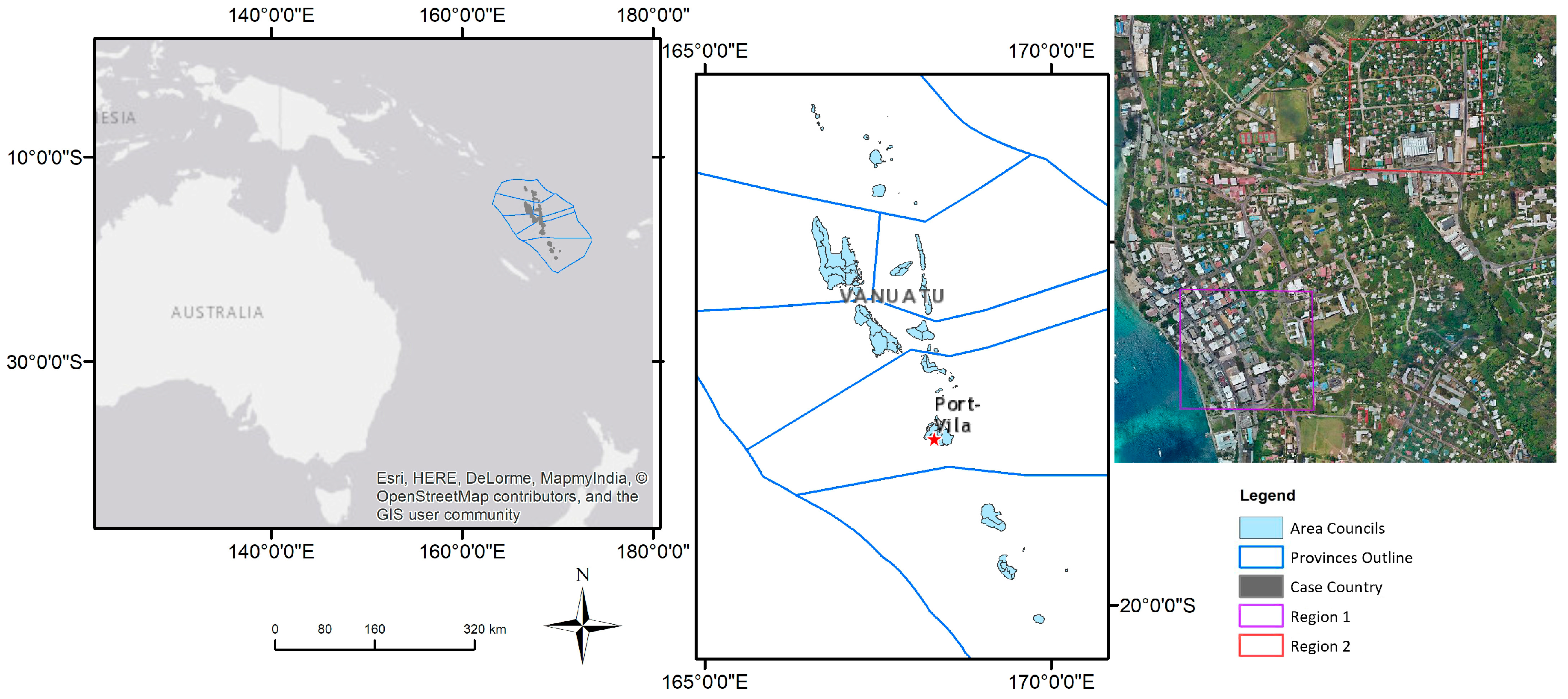
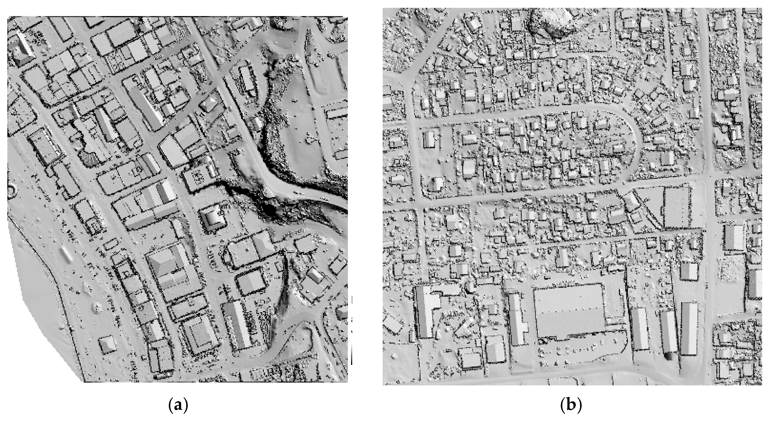
2.2. Study Area and Research Data

For the purposes of the study, the capital of Vanuatu, Port Vila was utilized. Vanuatu is a Y-shaped archipelago consisting of about 82 relatively small, volcanic origin islands [37]. Figure 1 gives an overall view of the territory of Port Vila as well as Vanuatu.
Vanuatu is an ideal case that has both cadastral and LiDAR data available. Moreover, the morphology in Vanuatu arguably provides an ideal representation of a developing, if not urbanizing, landscape, which is the target context of the overarching work. Lastly, initial investigations of the morphology of cadastral boundaries in Vanuatu supplies confidence on what to measure.
The capital, Port Vila in Efate, is covered by both ALS LiDAR data and a detailed cadastral map measured with DGPS—therefore, it was selected as the study area. The provided orthophoto was used as additional ground truth proving reference data. The coordinate system used in this study was UTM 59S, WGS 84.
The overall point density of the LiDAR data in Efate was 9.47 p/m2—a yield an accuracy of around 10 cm. According to the data quality report [38] the topography LiDAR points are classified into 9 classes, which is coherent with LAS standards [39].
Two regions in Port Vila were selected as the subset for further statistical analysis, one for the dense urban area and the other for the suburban area (Figure 1). From the orthophoto, these two regions are clear, with diverse land covers clearly distinguishable. They represent typical dense urban and suburban areas, respectively. Additionally, the research focus on general boundaries in the urban area, and the selected test regions, were both covered by the reference data. Separating these two regions enabled the study focus on the performance of the workflow on the diverse landscape of the urban area, in addition to shortening the processing time.

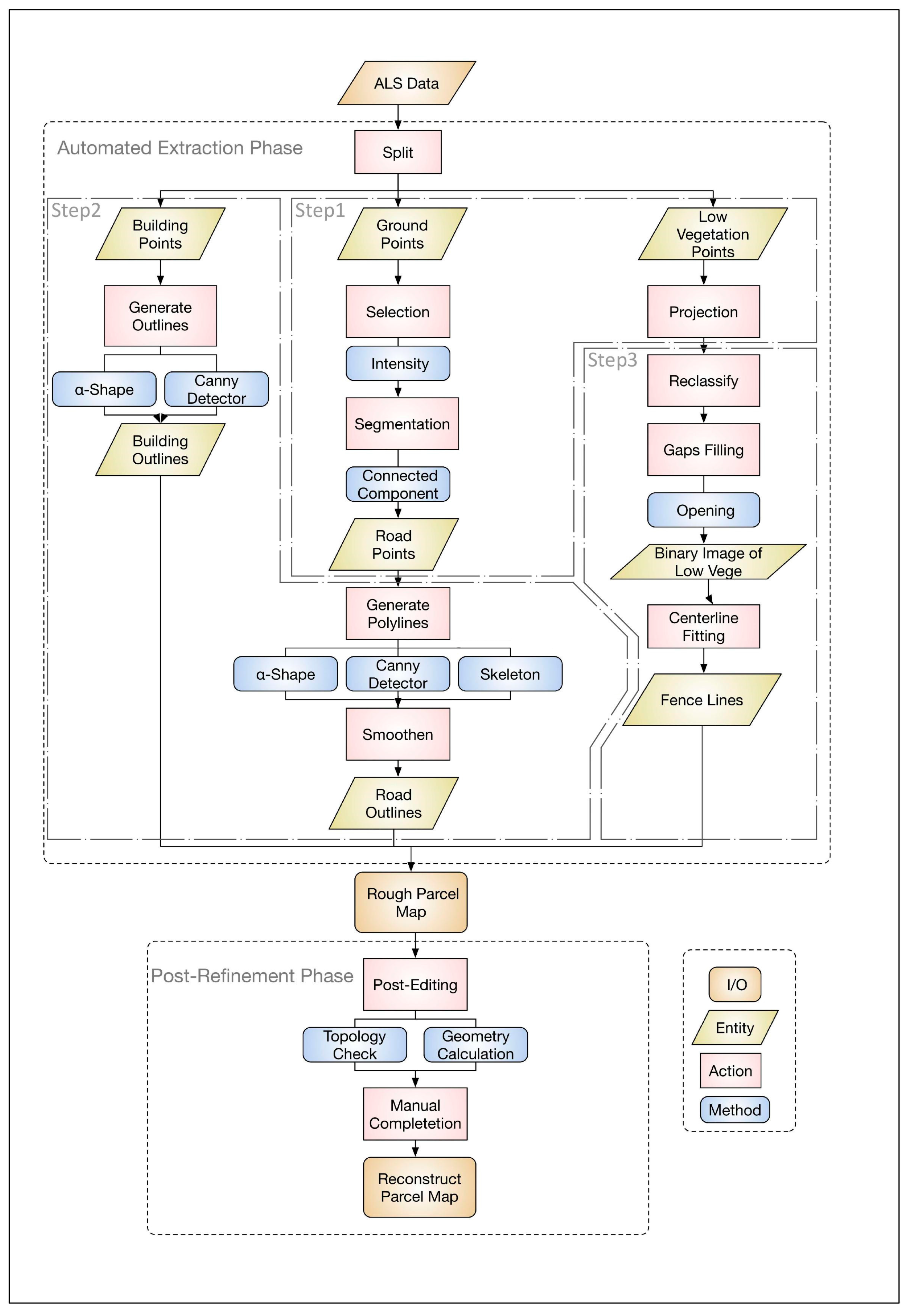
3. The Semi-Automated Workflow of Cadastral Boundaries Extraction

Based on the most prominent physic objects, namely roads, buildings, and fences, a workflow was developed to semi-automated extracting parcel boundaries.

3.1. Overview of the Semi-Automated Workflow

The developed workflow consisted of two phases: automated extraction and post-refinement. Three steps made up the automatic extraction phase: (1) classifying points into target objects; (2) generating planar object outlines—roads and buildings; (3) fitting centerlines to linear objects—fences.
Specific approaches were selected to conduct each step. In view of the complex morphology of cadastral boundaries, these approaches were able to deal with the large number of datasets, as well as with particular targets of the cadastral objects. Afterwards, extracted line segments were edited and completed in the post-refinement phase.
Diverse types of software were tested in different steps, in order to find an effective and efficient approach. Comparing the performance of each piece of software, with time and budget considered, the most suitable were determined for each step. Specifically, MATLAB executed outline generation algorithms because the tested algorithms were implemented in it. ArcScan was selected to achieve centerline fitting for its outstanding vectorizing function. LasTools was used to produce the hillshade images because it is the fastest solution for LiDAR data processing. CloudCompare, an open source and efficient software, was selected to conduct the segmentation and points filtering. Lastly, the well-known ArcGIS was used for output visualization and post-refinement. An overview of the extraction framework is given in Figure 2. It illustrates the designed steps and algorithms applied.

3.2. Further Classification for Expected Objects

The very first step of the workflow was to further classify points into target components, which were the road and fence in this study. Different methods were applied to recognize these two objects.

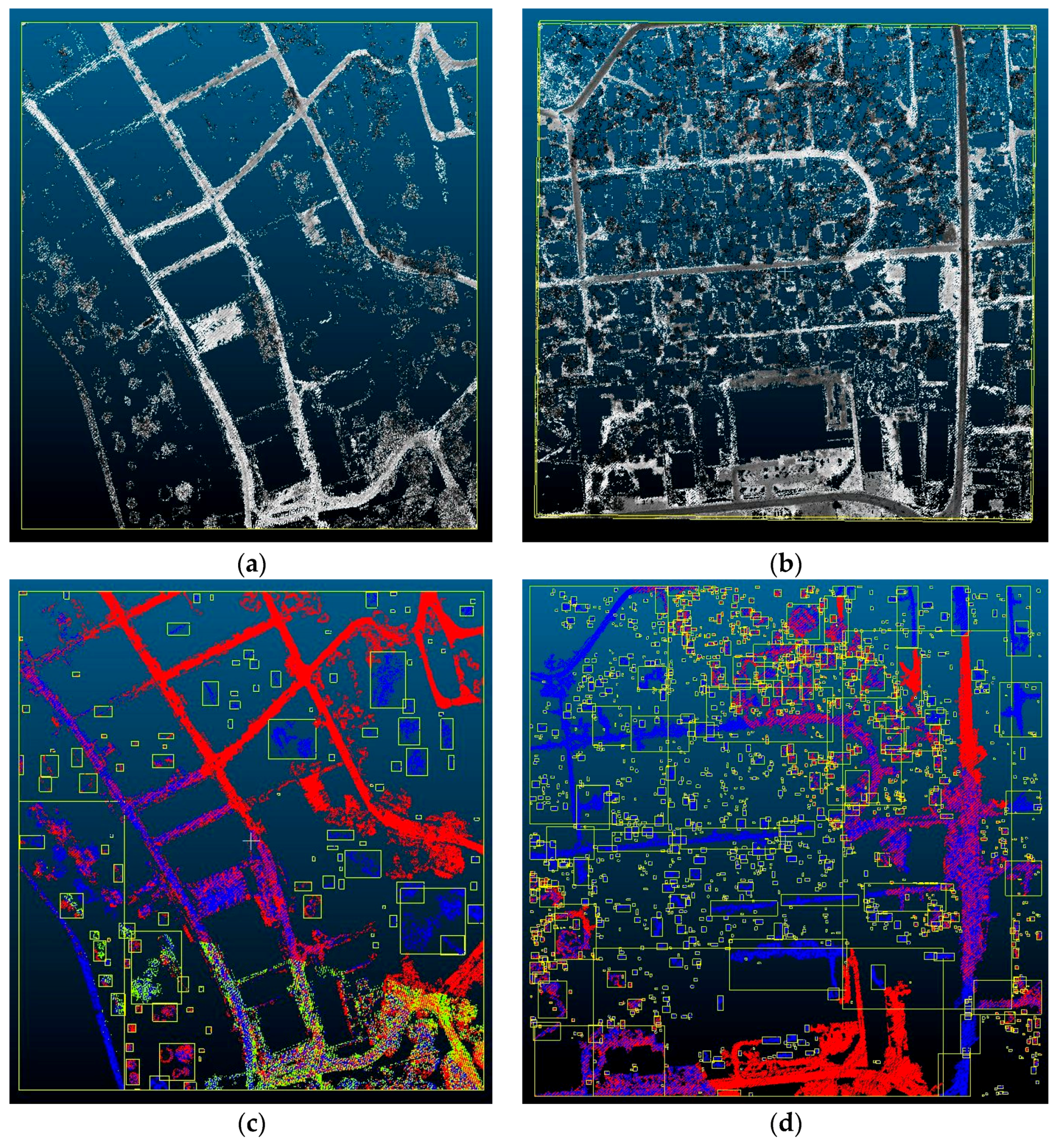
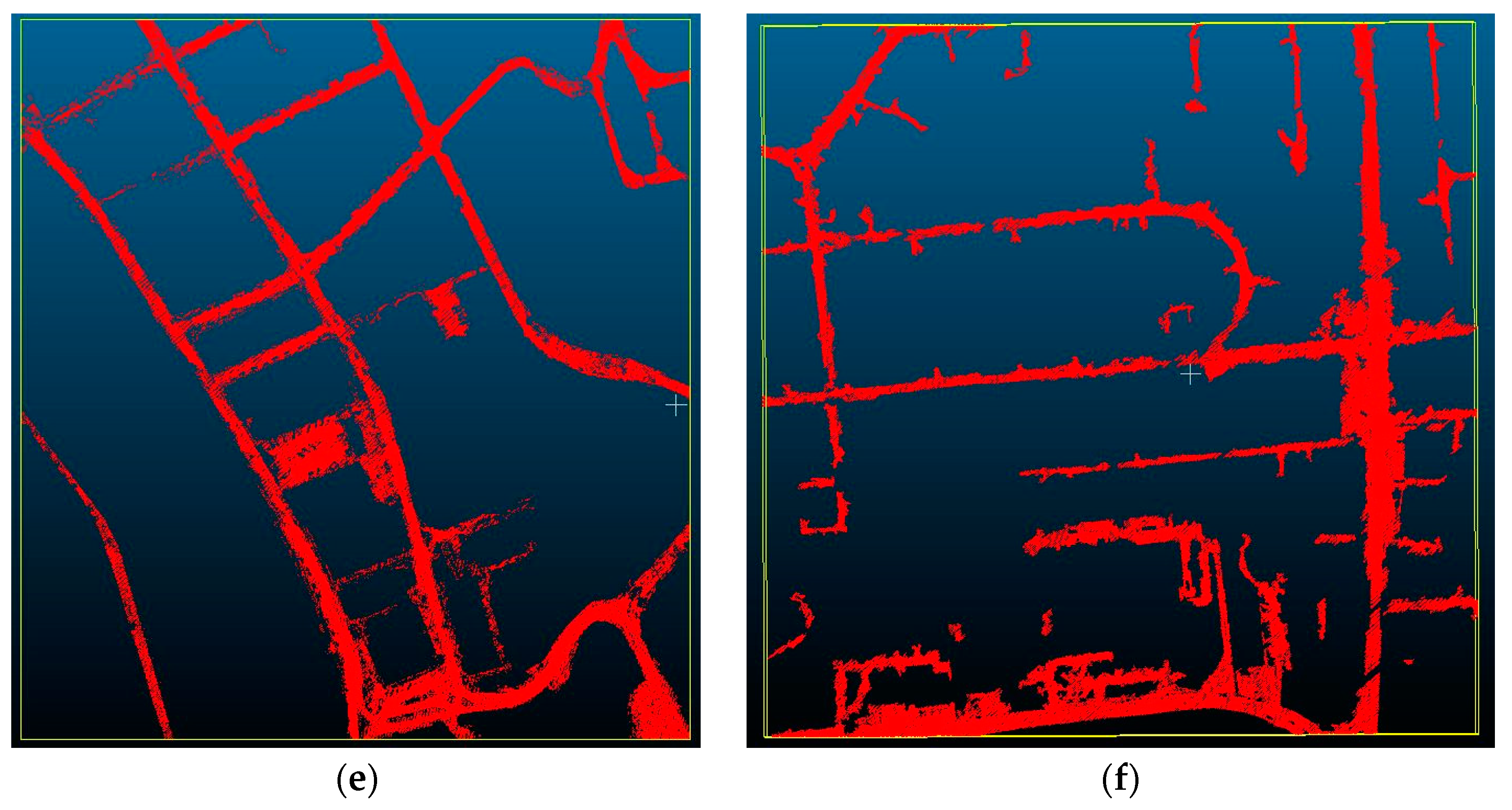
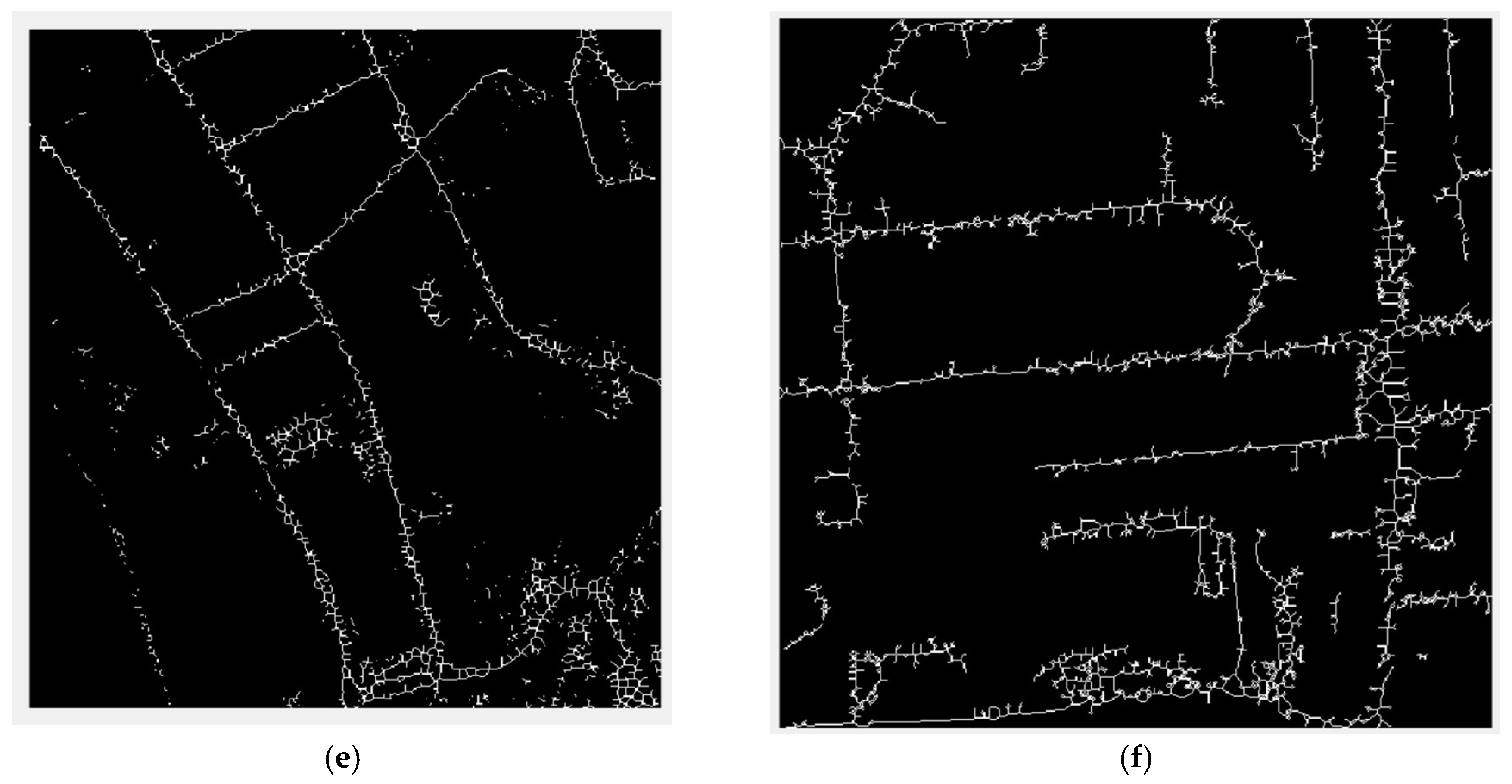
3.2.1. Road Detection from Ground Points

A cadastral boundary morphology study indicates that roads very likely coincide with cadastral boundaries [11]. Normally, roads lie at ground level and they cannot be separated by height differentiation. Inspired by the work of Clode, Kootsookos, and Rottensteiner [40], road material is usually uniform along a road section, in spite of the noisy value of intensity returned by scanning units. Therefore, points were then selected when their last pulse intensity values fell in the acceptable range for this type of road material. By searching for a particular intensity range (defined by Equation (1)), it is possible to extract most LiDAR points that were on roads, even though there were also some other on-road detections that were also produced. Equation (2) illustrates how the LiDAR points were filtered based on their intensity, in order to create a new subset of points [40].
S 1 = { P i S : i m i n < P i < i m a x }
where and i m i n and i m a x are the minimum and maximum acceptable LiDAR intensities at point Pi.
By visual interpretation, the intensity of road points in the two study regions was similar. This illustrated that in Port Vila, the material used in road constructions is uniform. The selected range was 0–25 and 30–55. The followed equation describes the road points subset S2.
S 2 = { P i S : 0 < P i < 25 | | 30 < P i < 55 } ,
Since roads are flat linear networks, they were assumed to be connected planes. After the points were selected, they were segmented by connected component analysis, based on planar distance among points. After the connected component segmentation, segments size was computed, and then small segments were defined as unvalued physical objects and removed. The remaining points were points on roads.
The result (Figure 3e,f) showed that some portion of roads were wrongly deducted, while some roadside bare lands still remained. Figure 3e (region 1) contains more irregular physical objects, while Figure 3f (region 2) presents a clearer linear road structure. This might be caused by more car parks and bare land in developed region 1, compared to region 2, where was covered by vegetation. Gaps exist in both regions, because of the wrong removal of small segments. Uneven points consequently distribute on the road surface in this incorrect segmentation.

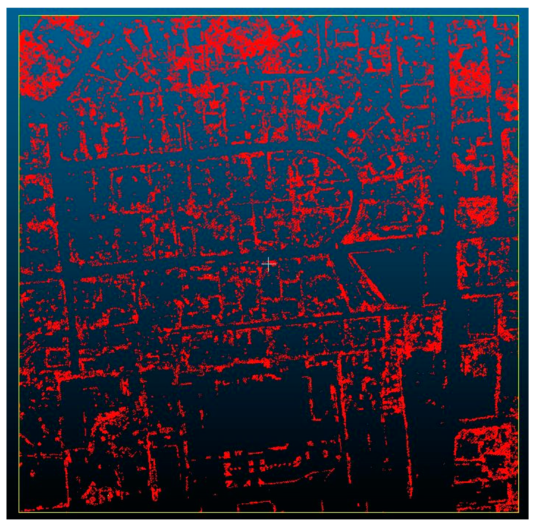
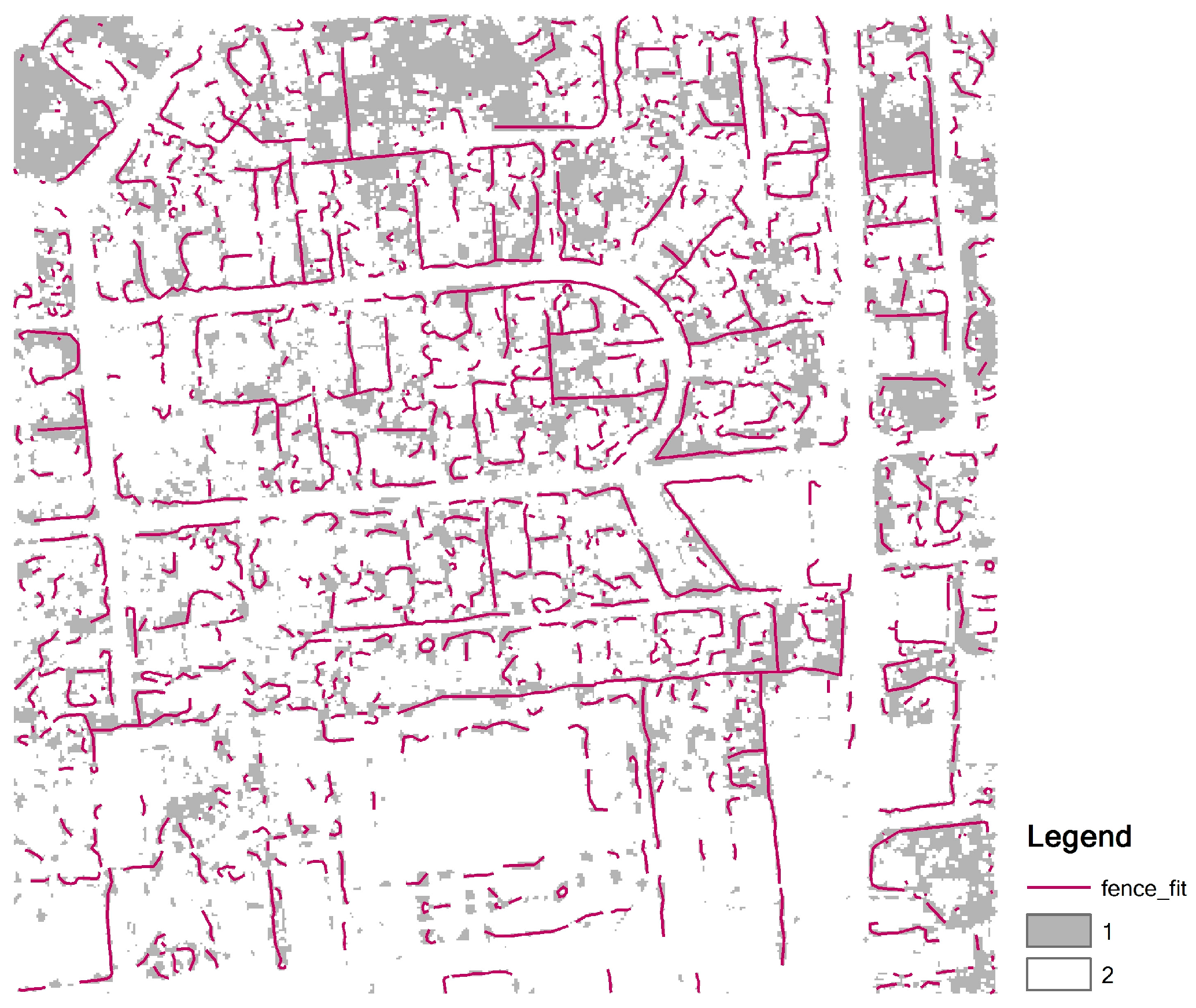
3.2.2. Fence Detection for Low Vegetation

In the suburban area, fences were the object that coincided the most with cadastral boundaries. However, they are hard to be distinguished from low vegetation: their heights were very similar. Furthermore, they cannot be computed from local smoothness, as they are too narrow to form planes. After eliminating classified building and ground points, the rest of the points were found to be composed of small structures like fences or vegetation.
Moreover, the material of the fence was uncertain: they may be made up by bush, concrete, or wood. In addition, the spectral information provided by LiDAR data over thestudy area was insufficient for recognizing fences. Except from reflectance intensity, an extra criterion—local point distance—was computed. The threshold was set to 1 pixel and standard deviation was computed of 6 neighbourhood points; afterwards, sporadic points were removed. However, as shown in Figure 4, the detection performance was better.
From the very general view on region 2, a rough impression of parcels can be identified. Some building edge points remain, as they were misclassified. Further, in denser vegetation cover areas, parcels cannot be distinguished.

3.3. Complemented Knowledge from Height Jumps

A complementary procedure was tested to delineate the outline of objects from height information. This supplementary process provided more knowledge on parcels boundaries, in cases where the topography relief resulted in incorrect detection. Hillshading was applied to visualize the height difference in this step. LAStools, a commercial software tool, was applied to conduct this process.
As illustrated as Figure 5, in region 1, building outlines were highlighted. Specifically, very closed building roofs were distinguished, as they were at different heights. The topography relief was also visible, which aids in separating road plane with roadside slopes. On the contrary, in region 2, whose topography is a flatter, hillshade visualization did not add much value. Even though building roofs were also highlighted, dense low vegetation was also mixed inside and ended up as noise.

3.4. Outline Generation of Detected Planar Objects

After the recognition of roads and fences, points were classified into target objects; the second step of the automatic extraction phase was to derive outlines from planar objects. According to the nature of objects, the physical objects were either planar or linear. The boundary approach was applied in planar objects such as building roofs, while the line fitting approach was more suitable for linear objects such as fences. However, roads lay between these two types of physical objects; therefore, both approaches were tested on roads. The following contents describe the process and results of each algorithm tested in the outline delineation of planar objects, the preliminary step for vectorization of boundaries from objects. A number of approaches were tested, including α-shape, Canny detector, and Skeleton. Though some of them worked on very regular contexts, most of them were found to not perform adequately.

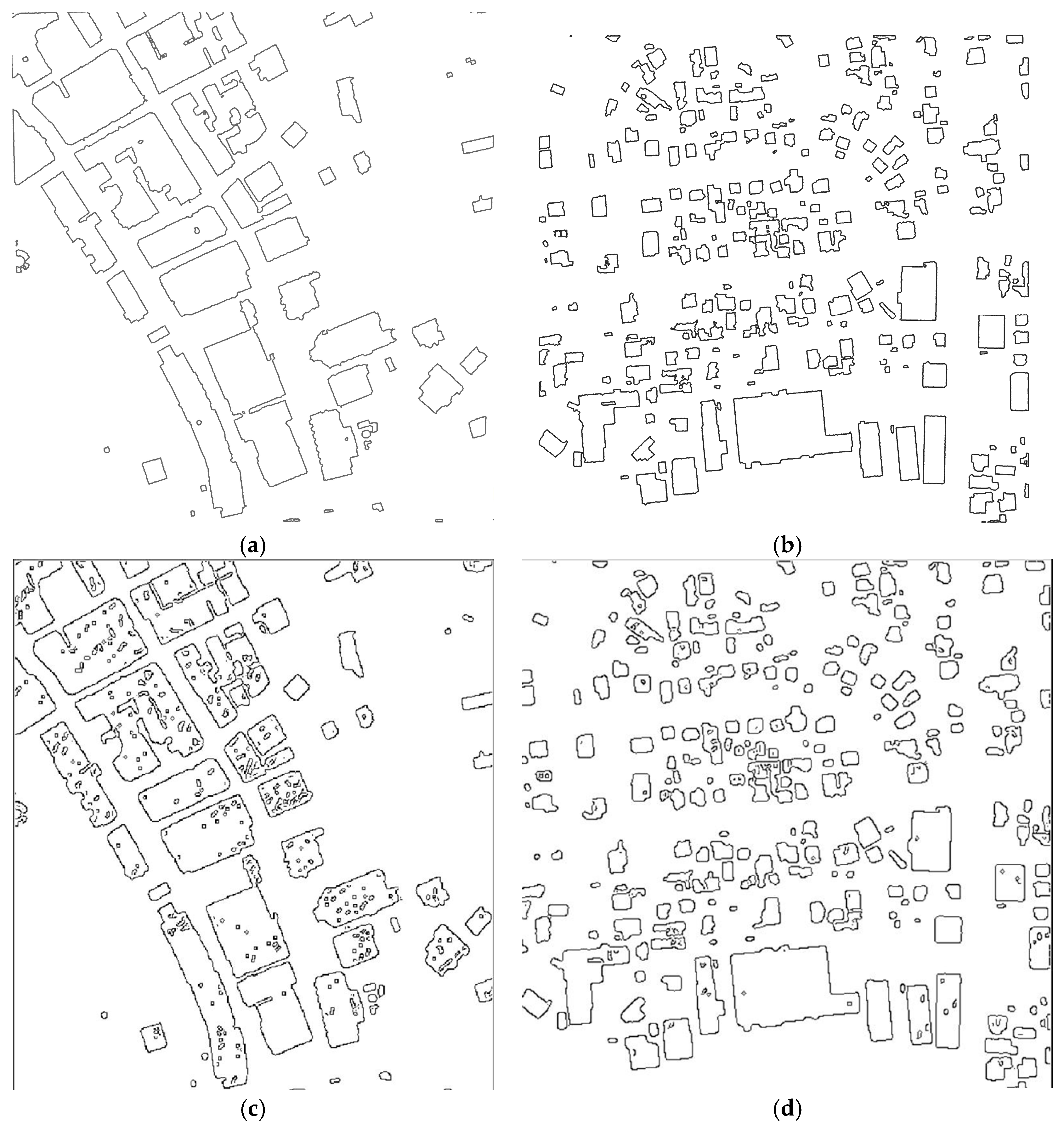
3.4.1. Building Outlines Extraction

A subset of building roof points was separated. The α-shape and Canny detector were tested for building outline generation (the results are shown in Figure 6). When testing α-shape, the radius was set to 1 in both regions, in order to acquire the best-fit and appropriately detailed outlines. In region 1, less vegetation mixed with roof edges, resulting in the shape of points being comparatively regular, and straight outlines. However, region 1 also has higher density construction, with buildings close to each other; therefore, they were difficult to separate.
Buildings in region 2 were sporadically mixed with low vegetation, with their borders covered. As a consequence, though building roof outlines were not as regular as in area 1, they were better separated.
The Canny algorithm is widely applied in the image processing field. Building points were projected on raster images, with pixel size equal to point space. It provided a similar result to α-shape. However, the extra rasterizing step introduced a decrease in the resolution. The edges were not as sharp as the result of the α-shape. Especially in region 2, small constructions lost their original shape. The most obvious error produced by the Canny algorithm was the small dots inside buildings and this may be originated from uneven point densities. Therefore, in this study, α-shape was adopted.

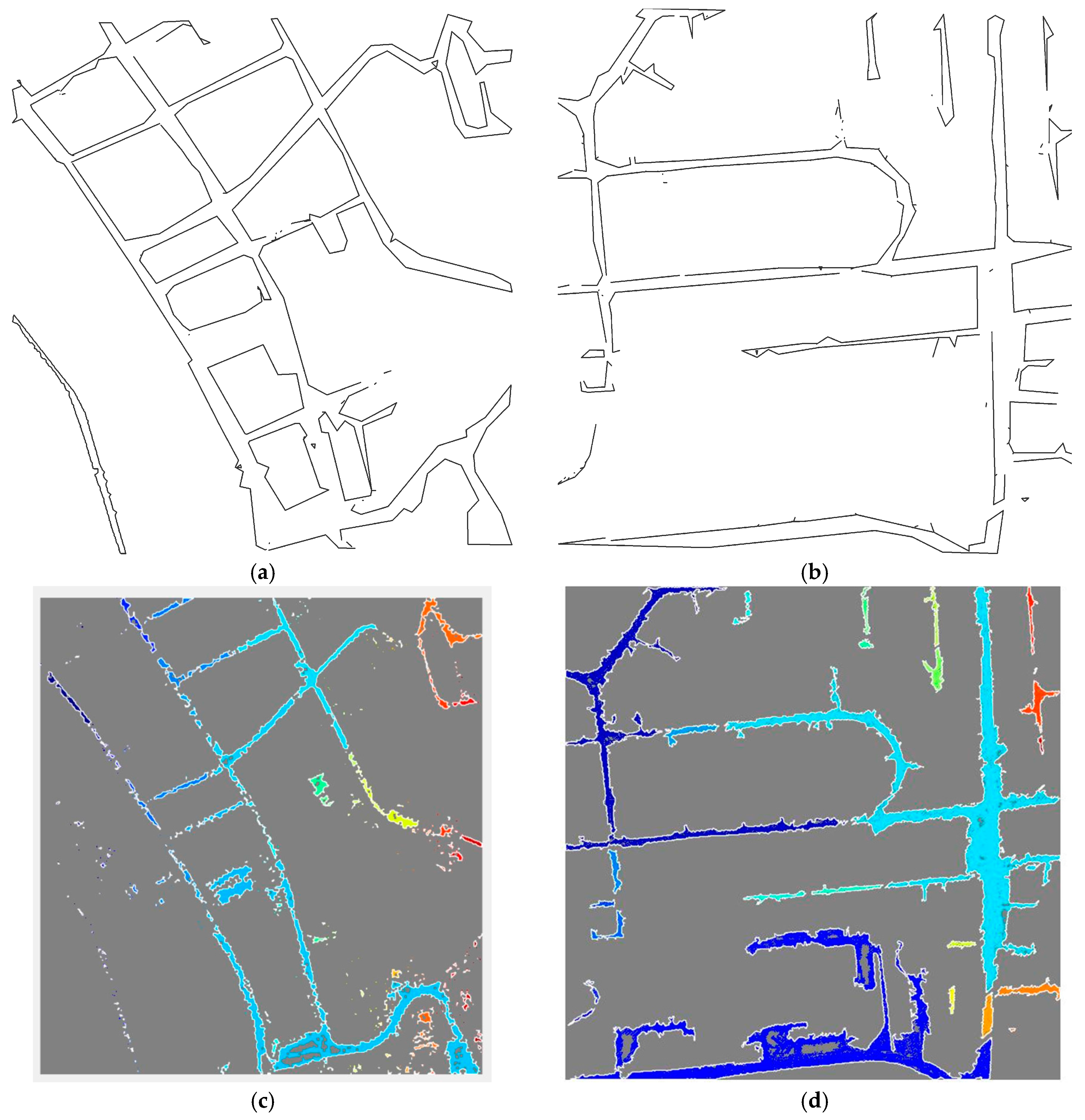
3.4.2. Road Outlines Extraction

Roads lie between planar or linear constructs. α-shape and Canny were applied to generate road outlines, while Skeleton was used to detect road trend. Due to the coarse road point classification, the shapes of roads were irregular. When generating road outlines, noisy objects were also included, and this resulted in zigzag outlines. The α-shape produced a detailed road outline map that described the roadside objects (Figure 7a). For both regions, the radius was set to 1.6, in order find a balance between straightening lines and maintaining details. Specifically, in region 1, the shape of roads on the slope was odd. On the other hand, since the width of roads in region 2 was smaller than in region 1, disconnects occurred with smaller radius (however, enlarging the radius setting would have resulted in a loss of detail).
Figure 7b displays the result of the outline generated by the Canny algorithm. A Gaussian blur was integrated before the computation of Canny, in order to decrease the thickness of roads. The process helped in removing the noisy roadside objects, though it also introduced disconnection. The Canny outline computed the concave hull of road segments, excluding small gaps inside the road surface. In both regions, the performance of the Canny algorithm depended mostly on the quality of the classification of road points.
Skeleton created rough centerlines of roads (Figure 7e,f). Though an impress of road network was clear visible, the width of roads was lost. As parcel boundaries usually coincide with road edges—the role of the road width and edges cannot be overlooked—this method therefore has limitations. In addition, line segments generated by skeleton were unconnected, and further simplification is required.
Comparing different approaches, the α-shape algorithm was the most suitable for road generation. The zigzag outlines were simplified and straightened in GIS environment (Figure 7), and the maximum acceptable distance was set to 2 m in both regions.

3.5. Line Fitting From Linear Fences

The last step for the automatic extraction phase was delineating lines from linear objects. ArcScan has a centerline fitting function: it can vectorize lines by tracing pixels. The roughly classified fence points were projected onto raster images. Pixels were reclassified into two classes: foreground and ground level. Line fitting was conducted on foreground pixels.
Before operating the line-fitting progress, an opening pre-processing was applied to fill in the small gaps. Afterwards, raster clearance removed single points by calculating the local stand deviation of point distances.
Line fitting results are shown in Figure 8a. Both centerline and outline were generated. Obviously, certain percentages of fence centerlines were drawn. The overview of parcels was vectorized into a polyline. Disconnecting pixels produced many very short line segments (shorter than 2 m), and they were unvalued noise.
A similar approach was conducted in hillshade images of region 1, to generate topography relief and building outlines. Since building outline generation from points cannot be separated from close buildings, this results in a more detail building interpretation. In region 1, building walls coincide with a large portion of cadastral boundaries. Therefore, it was necessary to ensure a more detailed building outline.

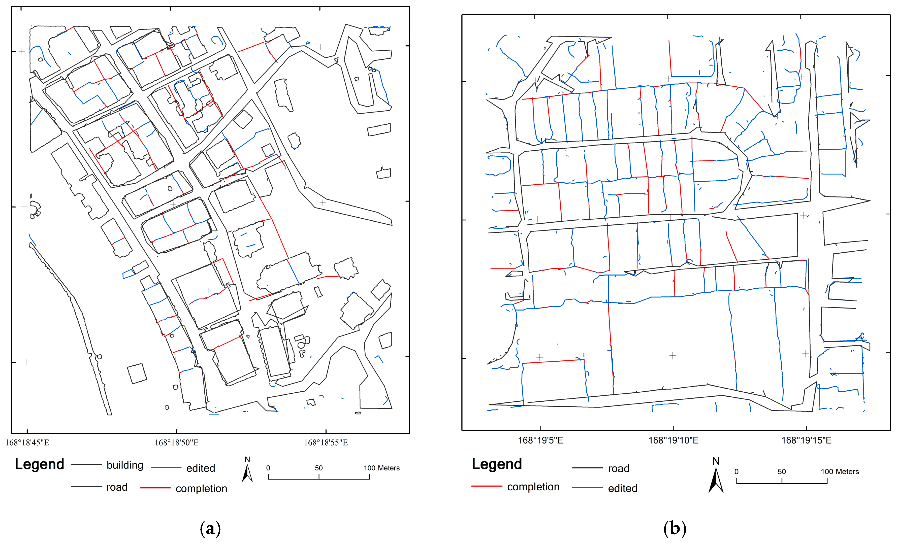
3.6. Reconstructing the Parcel Map by Post-Refinement

When rough lines had been generated by the automatic extraction phase, the results were further refined by the second phase of the workflow: post-refinement phase.
When overlaying all the automated extracted results with the orthophoto mosaic (the study regions’ cadastral situation), obvious mismatches between road boundaries and fitted lines emerged in both regions, due to the road thickness deduction along extraction. Furthermore, fitting lines and building outlines provide much more detail than roads boundaries. Generally, building outlines coincided with fitted lines, illustrating that the building extraction process approximately maintains the original shapes. However, the centerline-fitting approach produced a large number of short line segments. It was difficult to judge whether these sporadic short lines were meaningful.
In region 1, the fitted line of the hillshade visualization serves as complementary for distinguishing building blocks. However, as a highly developed area, morphology of parcels in region 1 is so irregular that it was hard to define the lines that are likely to coincide with cadastral boundaries. In region 2, where the majority of cadastral boundaries were composed of fence and road, building outlines serve as a supplement for defining parcel locations. In particular, when determining useful lines from line clusters, parcel boundaries normally surround buildings, rather than cutting through them.
After acquiring general knowledge from the automated extraction results, manual editing was conducted to reconstruct a rough parcel map. Different strategies were designed for the two regions.
An overall reorganization of the detected lines was preliminarily conducted on both regions. With a topology check, close and intersecting lines were merged. In the post refinement phase, less editing was executed on automatically extracted building outlines and road outlines, because they had higher positional accuracy.
The editing was mainly conducted on fitted lines. In region 1, a topology check was used to search for fitted lines that coincide with building boundaries: they were removed because of redundancy. On the other hand, the left fitted lines created from gaps between buildings or topography reliefs were kept. Comparatively, in region 2, portions of the fitted lines were generated from roadsides, in spite of fence centerlines. Topology was also applied to remove this redundancy. Afterwards, the length of the fitted lines was computed as a line attribute: line segments shorter than 2 m were removed. Based on the target feature strategy, a different combination of object lines was applied in the two regions. The rough parcel map of region 1 consisted of automatically extracted road outlines, building outlines, and edited fitted lines from hillshade visualization. Meanwhile, for region 2, the automatically extracted road outlines and edited fence fitted lines were grouped.
Manual completion was the final step for scene clearance. After determining the useful line segments with the help of visual interpretation, gaps among these line segments were manually filled in and short lines connected. Partition lines were created on the place where there were thought to be parcel boundaries. The final vector draft parcel maps of two regions are shown as Figure 9, respectively, edited lines are automated extracted lines but have been corrected or changed, while completion refers to lines that manually added. The whole manual editing process took less than half an hour to complete.
Generally speaking, for maintaining the research objective, in the post-refinement step, uncertain errors were left maintained, and only obvious and identifiable errors were edited. Certain rules were designed for this post-refinement. For instance, when editing road outlines, the over simplified sharp corners were left, but when the shape of roads were irregular rather than linear, these parts were removed. In terms of centerline fitting, for both the building gaps fitting in region 1 and the fence fitting in region 2, majority edits were made when encounter following two conditions. The first related to the angle between line segments. That is, the angle needed to be larger than a certain about of degrees (e.g., 75), because parcel corners are not likely to be too acute. The other condition was when the endpoint of a line segment was close to an intersection. In addition, if line segments were randomly orientated or sporadically distributed, they were removed.

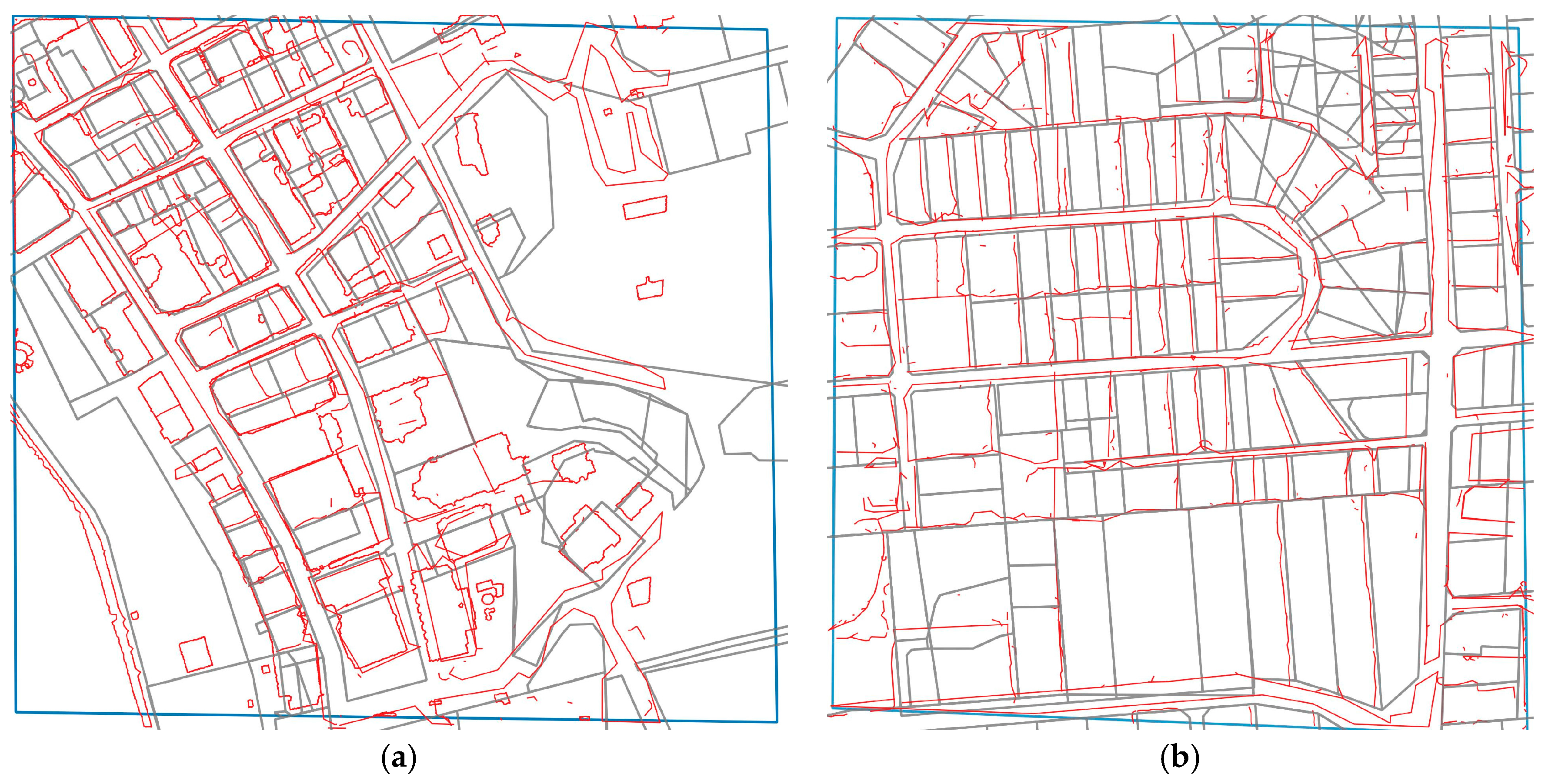
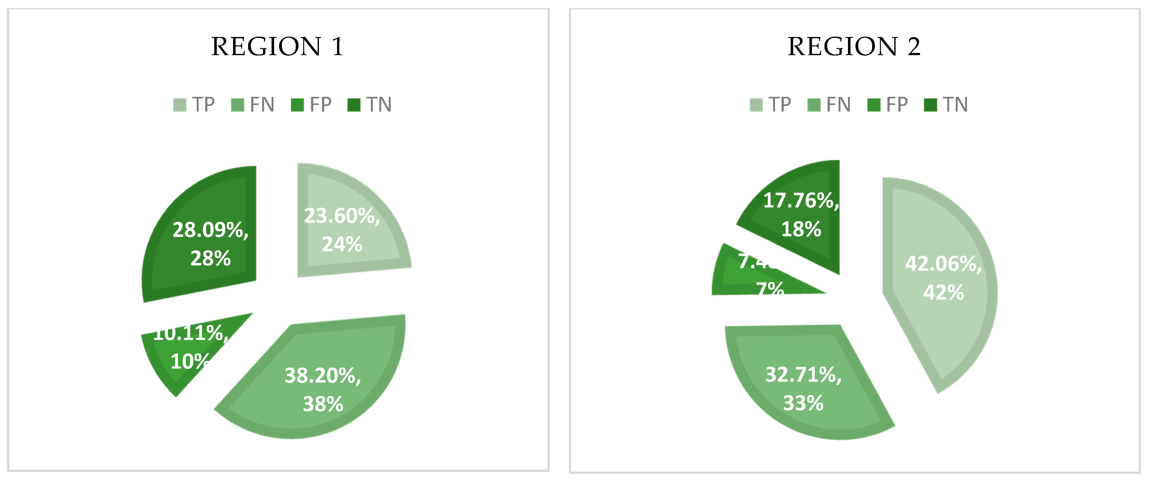
4. Workflow Performance Evaluation

4.1. Comparison with Exiting Cadastral Map

The evaluation stage compared the extracted results of both phases with reference data, the cadastral map, and made assessment in terms of the correctness and completeness of the developed workflow. Figure 10 provides an overview of the workflow performance. There is a small portion of reconstructed lines that completely coincide with ground truth, whilst the others possess errors like offsets and wrong detections. The error sources, as well as tolerances, will be described now.
Obviously, the workflow performs better in region 2 than region 1. In region 2, the scene is clearer with less disruptive lines, while on the contrary, in region 1, redundant and single stand lines exist. Cadastral morphology is indeterminate in dense urban areas. For instance, when a block consists of a couple of parcels, the outer parcel boundaries normally coincide with roads surrounding the block. However, the interdivisional lines normally cut through building gaps. Nevertheless, in dense urban areas, buildings often adjoin to roads: more efficient land use is caused by higher land price. Thus, when the workflow extracts both buildings and roads outlines, a certain redundancy occurs on block outlines. On the other hand, the parcel shape and size are not uniform—for example, some parcels possess more than one building, some parcels are larger, and the others are smaller. This phenomenon contributes difficulties to the boundary location prediction. Therefore, diverse noise made the overall result of region 1 looks coarser.
Comparatively, the scene of region 2 is cleaner. There are more recognizable parcels in the scene. Similar to region 1, blocks are separated by roads outlines. Within blocks, parcels are regularly arranged with evenly distributed areas. Most parcels are rectangle and north orientated. Though fences were hardly seen from images when they were covered by vegetation, the workflow filtered out the high vegetation and fences mixed with the low vegetation were then left. They serve as markers describing the range of land parcels. However, in real-life situations, boundaries do not always cut through the middle of thick brush, therefore there are obvious offsets existing between extracted fence lines and the reference data. In general, the fitted centerline partly draws the division boundaries.

4.2. Error and Tolerance

As described previously, extracted lines are not totally aligned with the ground truth. Errors can be summarized into three categories, by their sources and appearance. One is raised from outlines generation; the second presented as offset; and the third is caused by misalignment between features and cadastral boundaries. By studying the characteristics of errors, standards for the result evaluation were defined based on whether the error can be improved. Tolerance was determined according to the maximum distance between extracted lines and relative reference data. If errors can be eliminated through further improvement, they were recognized as acceptable.
The coarse outline extraction introduced errors when connecting boundary points. Especially in road outline generation, the reducing approach incorrectly subtracted points on roads, as well as decreasing the road’s thickness. Though a simplification step was integrated, it also brought noises through over-simplification. As shown in Figure 10a, the roads width was decreased and the shape of some corners were lost. A better threshold for straighter and simplified road outlines should have been investigated.
If the maximum distance to reference data is smaller than 4 m, which is approximately one third of the road width, the extraction was recognized as correct: in general less accuracy is required in general boundary surveys. However, if the maximum distance is too large, though they were correctly extracted from features, they were determined as errors.
The most common error cause was the offset between the extraction result and reference data. Offsets occur in both building outlines and fence fitting lines, but the causes for both were different. No systematic shift was observed between these two datasets, and the causes of the offset might be dynamic. In region 1, building outlines were shifted at certain angles, and this might be caused by the vague edge of building points. In region 2, probably because not all cadastral boundaries cut through the center of fences, offsets exist between the extracted result and reference data. Fortunately, the thickness of brushwood and fences are small enough to control the maximum shift distance.
Similar to the previous type of error, when the average distance between the extraction result and the reference data was smaller than one third of road width, errors were considered within tolerance. Otherwise, they were recognized as unvalued.
In reality, there are certain percentages of parcel boundaries that are neither coincidental with any features, nor visible by human eyes. Conversely, these feature outlines may represent no parcel boundaries. Simply improving extraction techniques cannot decrease this type of error. More intelligent approaches should be integrated to mitigate human definition of cadastral boundaries. Thus, this type of errors falls outside tolerance.

4.3. Workflow Correctness and Completeness

Since errors and tolerance were determined, the performance could be quantitatively evaluated by statistical analysis. The percentage of correctly extracted lines and the proportion of detected parcels were selected as measures to describe the completeness of the designed workflow. Correctness is illustrated by the percentage of correct extraction from the total number of extracted lines.

4.3.1. Proportion of Detected Lines from Each Kind of Feature

Table 1 describes the number of both true and false line segments from total extracted lines. Road extraction was conducted on both regions: building outlines and fence fitting were executed in region 1 and region 2, respectively. The total number of extracted line segments was counted. True lines are extracted lines that coincide with relative cadastral boundaries, while false lines are either wrongly detected or their error are larger than tolerance.
The correctness was computed as a percentage of true line segments from total extraction in each region. The completeness refers to the ratio of correctly extracted lines segments to the total cadastral boundary segments in each region. In region 1, a total of 54.32% of extraction are true, whilst this number rises to 84.1% in region 2. Completeness was computed by the percentage of extracted line segments from detectable boundaries (Table 2).
Specifically, Table 2 indicates a very low contact ratio on building outlines, which also reveals the complicated cadastral boundary morphology in urban areas. The fence fitting realized the highest correctness in this study.

4.3.2. Performance of Full Parcel Identification

The Table 3 illustrates the fully detected parcel. Identifiable parcels are parcels where all their boundary segments have been extracted. It is illustrated that the ratio of identified parcels of region 2 is almost double that of region 1. ‘Shifted’ parcels refers to those extracted parcels, that are significantly shifted from reference position. The workflow extracted less shifted parcels from region 2 than from region 1, reflecting that the workflow performed higher positional precision in a more regular area.
Figure 11 displays a straightforward illustration on parcels identification. It uses true, false, positive, and negative to summarize the overall performance on the parcel extraction. TP refers to parcels appearing in both extracted results and reference data. FP refers to where parcels were in reference data, but were not extracted. FN refers to those parcels that appear in the result, but do not exist in reference data. Lastly, TN refers to those parcels from the reference data that were only partly extracted or had a visible shift. TP describes the completeness of the parcel identification, and both regions achieved less than half, with region 1 having even less.

4.4. Degree of Automation

Two phases of the semi-automated workflow were separately evaluated, in order to assess the workflow’s degree of automation. Firstly, the total length of the line segments generated in both automatic extraction and post-refinement phase were computed. Then, the correctness of each phase was assessed respectively. The results indicated that the workflow performed better in region 2 in either phase. Table 4 illustrates the different performance of the workflow in two regions.
In Region 1, the workflow was conducted on the two highest probability features—roads and buildings—and this achieved both approximately two-thirds correctness. Without ground reference, it is hard to judge whether extracted lines from road points are correct or not. Therefore, for maintaining this experiment objectivity, in the post-refinement step, uncertain errors were left maintained, and only obvious and identifiable errors were edited.
Equation (3) calculates the degree of automation D, where the total length is the total length of workflow result that consists of automated extraction result and post-refinement result; automated extraction is the total length of the automated extraction phase result that have been used for reconstruction. In this study, in region 1, automated extraction results of road and building outlines were used, whereas in region 2, only road outlines were used, and all fence fitted lines were edited.
D = A u t o m a t e d   E x t r a c t e d T o t a l   L e n g t h * 100 %
The automation degree of workflow in region 1 is 89.3%, and the number drops to 45.75% in region 2. This slight difference is caused by more unpredictable parcel morphology in the dense urban area, which is region 1 in this study. It was difficult to judge whether an extracted line in region 1 is valuable. As a consequence, in many cases, errors were maintained with less manual editing. Comparatively, the fence-fitting result was coarse and all of them have been manually inspected.
From another perspective, the post refinement phase achieved higher correctness in region 2 than in region 1. It further proves that without reference, regular parcel shape and uniform parcel size would contribute to correctness of the post-refinement activities. That is, human interpretation highly depends on these regular patterns.

4.5. Suitable Point Density for Target Objects

Observed from the result, some skinny stand-alone parcel boundaries cannot be detected from lower density point clouds. Therefore, a suitable point density should be defined in advance, according to the accuracy requirement of cadastral surveys. After defining the target objects, the Equation (4) adapted from the Nyquist Sampling equation determined a suitable point cloud, to inspect the capability of study data. The smallest dimension of a particular object in a point cloud was used to determine the minimum point cloud density for detecting that particular object. When determining the smallest dimension of a target object from the nadir view, only the width and length of objects were considered. The point spacing should be smaller than the smallest object dimension.
p = 1 ( s m a l l e s t   o b j e c t   d i m e n s i o n / 2 ) 2
In this study, the thinnest target object is the fence. Normally, the width of the fence is 0.5 m, thus, the smallest point cloud density for detecting the fence is 16 points per square meter (p/m2). However, the point density of the study data is only 9 p/m2: the smallest detectable dimension is 1.3 m, smaller objects like the fence may be undetectable in this study, while others are larger than the minima. Although in reality, very thin and long objects still have possibility to be seen from point cloud, because points are regularly arranged.
Obviously, a higher point cloud density would have helped to detect more fences. Though higher point density provides more details, it also costs more. Thus, appropriate data volume should be investigated based on the fit-for-purpose concept.

5. Discussion

5.1. Observations from the Workflow Development

After exploring the proposed workflow, the α-shape algorithm was adopted for both building outline and road outline generation. Since this study aimed to the reconstruct a 2D cadastral map, only planar coordinates of points were taken into consideration. However, this manner introduces errors, in that different roof planes cannot be separated from different heights. Additionally, in many cases, close building roofs were wrongly segmented into one cluster, in that the gaps among buildings are too thin to be separated. The accuracy of the α-shape algorithm highly depends on point cloud segmentation quality, because it connects all boundary points of a segment to construct the boundary polyline. As a result, when generating building outlines in the urban area, close building roofs were wrongly merged into one polygon.
In terms of the road point classification, the quality was restricted by the limited spectral information of point clouds. The LiDAR data in this study works on one band, which offers much less spectrum information than multi-spectral images. The workflow detected points of roads from its intensity, however, the reflectance from road surface and roadside constructions are too similar, so incorrect detections occured along the roadside. A fusion of point clouds and multi spectral images might provide a better quality result.
The evaluation results indicate that the workflow performed better in the more regular suburban area. Therefore, the workflow performs better in regular contexts: parcel morphology plays an important role in extracting boundaries. However, the complex parcel morphology in the dense urban area created difficulties in parcel boundaries delineation. As an exploratory approach, the tolerance was set modestly, which was significantly larger than most cadastral survey requirements, with the concept of realistic boundary and general boundary taken into consideration.

5.2. Strenghts and Limitation

LiDAR data possesses both strengths and weakness with respect to cadastral purposes, and the workflow explored the feasibility of LiDAR applied to cadastral surveys. The most significant advantage is its ability to penetrate through a vegetation canopy, which contributes much to the fence extraction. Fences are widely-used as cadastral markers, but they are often invisible from aerial images. Although there is high vegetation covering above, laser beams can penetrate through the canopies and return footprints of objects below high vegetation, which in this study was the low ‘mixed vegetation’fences. Another strength of using LiDAR is that it provides height information. Point cloud data can provide high accuracy XYZ measurements. Height plays an important role in objects recognition. On the contrary, the major weakness of using point clouds is its accuracy. The level of detail that LiDAR can provide is highly dependent on the point cloud density. Extracting small objects such as fences occurring in the test site requires a higher point density, but, of course, a higher point density also means a larger data size, as well as higher costs of data acquisition. This is a disadvantage in application in developing countries, where cost remains a primary concern and inhibitor.
Since a cadastral boundary is a societal construct, manual verification can be largely reduced through semi-automated extraction, rather than eliminated totally. However, not all cadastral boundaries are visible, and not all objects coincide with cadastral boundaries. Therefore, it was hard to judge whether the lines are valuable, and in consequence, redundancy and incompleteness are inevitable during the whole workflow. Whether the accuracy of automated extraction meets the requirement of cadastral survey needs a quantifiable justification.
In view of the strengths and weakness of the workflow, several recommendations are derived for improvement. The first one is to improve the feature extraction approach. A constraint that restricts the road width was not integrated into this workflow. By computing the distance between points, a fixed width road surface can be formed and then the ‘zigzag’ outline problem may be solved. In addition, when generating building outlines, the workflow only considered the xy coordinates. If the α-shape algorithm is extended to 3D, close roof planes can be separated by their different heights. Furthermore, a combination of multi-spectral images can enrich spectral information and makes a contribution to point-based classification. The third recommendation is to automate the post-refinement phase. This can be achieved by integrating them into line generation. Taking a topology check and the line simplification as an example, if they can be executed during the generation of lines, not only can much person power could be saved, but also the whole workflow would be accelerated.
Another suggestion for improvement would be to adapt the object-based approach to investigate the relationship between objects and parcel boundaries, such as the possible distance between constructions and parcel boundaries. In urban areas, cadastral boundaries may be close to a building outline; whilst in suburb areas, cadastral boundaries may evenly partition an area. These parameters could be taken into consideration for predicting parcel range and location by means of machine learning. These conjectures could contribute to a future research prospect.

6. Conclusions

This study, which explored the feasibility of point cloud data for cadastral survey, achieved the main objective: to develop a workflow for semi-automated extraction of cadastral boundaries from airborne laser scanning data. Port Vila of Vanuatu was selected as the study area, in order to investigate the capability of semi-automated cadastral mapping in a developing country context. The study focused on the visible general boundaries, through exploring suitable methods; an object-based workflow was developed to semi-automatically extract cadastral boundaries from ALS point clouds. The result of the developed workflow is promising, with around 50% of parcel boundaries successfully extracted. A coarse parcel map can be arranged with the workflow within several hours. If one brings the parcel map to field for verification, only incorrect boundaries need to be digitized afterwards. However, the spatial accuracy of this workflow is still modest, because most steps of the workflow introduce errors. Furthermore, the workflow is context specific. It was fortunate that in the study area, a large proportion of cadastral boundaries coincided with topographic objects. It may not be suitable for areas with irregularly shaped land holdings, such as dense slum areas:the workflow performed better in the more regular suburban area. Due to the complexity of the cadastral boundary morphology in the dense urban area, the performance of the workflow in the dense urban area is still modest. More research on the relationship between topographic objects and parcel boundaries deserves further exploration.

Acknowledgments

The author thank the CRC-SI, Australia, and in particular Nathan Quadros, for sharing his expansive knowledge on LiDAR surveys and feature extraction, and for coordinating access to ALS data from the case locations. Also thanks to John Meadows from Land Equity and the Land Administration Department of Vanuatu for supplying the reference cadastral data.

Author Contributions

Xianghuan Luo led on research execution and manuscript drafting. Designed methodology, conducted bulk of experimentation; organization of results and lead role in drafting manuscript; coordination of coauthors. Rohan Bennett generated main topic; defined and guided the overarching research approach; led on liaisons and agreements with data providers; guidance on data and analysis problems and questions; support on manuscript structuring, editing and refinement. Mila Koeva led on technical aspects and tool application; guided and assisted in designing a draining methodology and experiments; refine problems and questions; decision making; refine throughout the draft manuscript. Christiaan Lemmen guide the topic background and major approach; problems finding; modify concepts; refine throughout the manuscript.

Conflicts of Interest

The authors declare no conflict of interest.

References

  1. Enemark, S.; Bell, K.; Lemmen, C.; McLaren, R. Fit-for-Purpose Land Administration; No. 60; Joint FIG/World Bank Publication: Copenhagen, Denmark, 2014. [Google Scholar]
  2. Roger, J.; Kain, P.; Elizabeth, B. The Cadastral Map in the Service of the State: A History of Property Mapping; The University of Chicago Press: Chicago, IL, USA, 1992. [Google Scholar]
  3. Zevenbergen, J.; Augustinus, C. Designing a pro poor land recordation system. In Proceedings of the FIG Working Week, Marrakech, Morocco, 18–22 May 2011; pp. 18–22. [Google Scholar]
  4. Simbizi, M.C.D.; Bennett, R.M.; Zevenbergen, J. Land tenure security: Revisiting and refining the concept for Sub-Saharan Africa’s rural poor. Land Use Policy 2014, 36, 231–238. [Google Scholar] [CrossRef]
  5. Jochem, A.; Höfle, B.; Wichmann, V.; Rutzinger, M.; Zipf, A. Area-wide roof plane segmentation in airborne LiDAR point clouds. Comput. Environ. Urban. Syst. 2012, 36, 54–64. [Google Scholar] [CrossRef]
  6. Vosselman, G.; Dijkman, S. 3D Building Model reconstruction from point clouds and ground plans. Int. Arch. Photogramm. Remote Sens. 2001, XXXIV, 22–24. [Google Scholar]
  7. Yu, Y.; Li, J.; Member, S.; Guan, H.; Jia, F.; Wang, C. Learning hierarchical features for automated extraction of road markings from 3-D Mobile LiDAR point clouds. IEEE J. Sel. Top. Appl. Earth Obs. Remote Sens. 2015, 8, 709–726. [Google Scholar] [CrossRef]
  8. Monnier, F.; Vallet, B.; Soheilian, B. Trees detection from laser point clouds acquired in dense urban areas by a mobile mapping system. ISPRS Ann. Photogramm. Remote Sens. Spat. Inf. Sci. 2012, I-3, 245–250. [Google Scholar] [CrossRef]
  9. Van Beek, N. Using Airborne Laser Scanning for Deriving Topographic Features for the Purpose of General Boundary Based Cadastral Mapping. Master’s Thesis, University of Delft, Delft, The Netherlands, 2015. [Google Scholar]
  10. Crommelinck, S.; Bennett, R.; Gerke, M.; Nex, F.; Yang, M.Y.; Vosselman, G. Review of automatic feature extraction from high-resolution optical sensor data for UAV-based cadastral mapping. Remote Sens. 2016, 8, 689–717. [Google Scholar] [CrossRef]
  11. Luo, X. Cadastral boundaries from point clouds?: Towards semi-automated cadastral boundary extraction from ALS data. GIM Int. 2016, 30, 16–17. [Google Scholar]
  12. Dale, P.; McLaughlin, J. Land Administration; Oxford University Press: Oxford, UK, 2000. [Google Scholar]
  13. Zevenbergen, J. Systems of Land Registration, Aspects and Effects; NCC: Amersfoort, The Netherlands, 2002. [Google Scholar]
  14. Williamson, I.P. Land administration ‘best practice’ providing the infrastructure for land policy implementation. Land Use Policy 2001, 18, 297–307. [Google Scholar] [CrossRef]
  15. Abdulai, R.T.; Obeng-Odoom, F.; Ochieng, E.; Maliene, V. (Eds.) Real Estate, Construction and Economic Development in Emerging Market Economies; Routledge: Abingdon, Oxfordshire, UK, 2015. [Google Scholar]
  16. Bennett, R.; Alemie, B. Fit-for-purpose land administration: Lessons from urban and rural Ethiopia. Surv. Rev. 2016, 48, 11–20. [Google Scholar] [CrossRef]
  17. GLTN—Global Land Tool Network. 2016. Available online: http://www.gltn.net/index.php?option=com_content&view=article&id=437 (accessed on 4 February 2016).
  18. Robillard, W.; Brown, C.; Wilson, D. Brown’s Boundary Control and Legal Principles; Wiley: Hoboken, NJ, USA, 2003. [Google Scholar]
  19. Bruce, J.W. Review of tenure terminology. Tenure Br. 1998, 1, 1–8. [Google Scholar]
  20. Dale, P.; McLaughlin, J.D. Land Information Management an Introduction with Special Reference to Cadastral Problems in Developing Countries; Clarendon Press: Gloucestershire, UK, 1988. [Google Scholar]
  21. Tuladhar, A. Spatial cadastral boundary concepts and uncertainty in parcel-based information systems. Int. Arch. Photogramm. Remote Sens. 1996, 16, 890–893. [Google Scholar]
  22. Kern, P. Automated feature extration: A history. In Proceedings of the MAPPS/ASPRS 2006 Fall Conference, San Antonio, TX, USA, 6–10 November 2006. [Google Scholar]
  23. Overly, J.; Bodum, L.; Kjems, E. Automatic 3D building reconstruction from airborne laser scanning and cadastral data using Hough transform. Int. Arch. Photogramm. Remote Sens. Spat. Inf. Syst. 2004, 34, 296–301. [Google Scholar]
  24. Dorninger, P.; Pfeifer, N. A comprehensive automated 3D approach for building extraction, reconstruction, and regularization from airborne laser scanning point clouds. Sensors 2008, 8, 7323–7343. [Google Scholar] [CrossRef] [PubMed]
  25. Elberink, O.; J, S.; Vosselman, G. 3D information extraction from laser point clouds covering complex road junctions. Photogramm. Rec. 2009, 24, 23–36. [Google Scholar] [CrossRef]
  26. Sohn, G.; Jwa, Y.; Kim, H.B. Automatic powerline scene classification and reconstruction using airborne lidar data. ISPRS Ann. Photogramm. Remote Sens. Spat. Inf. Sci. 2012, I, 167–172. [Google Scholar] [CrossRef]
  27. Vosselman, G. Point cloud segmentation for urban scene classification. ISPRS Int. Arch. Photogramm. Remote Sens. Spat. Inf. Sci. 2013, XL-7/W2, 257–262. [Google Scholar] [CrossRef]
  28. Xu, S.; Vosselman, G.; Elberink, S.O. Multiple-entity based classification of airborne laser scanning data in urban areas. ISPRS J. Photogramm. Remote Sens. 2014, 88, 1–15. [Google Scholar] [CrossRef]
  29. Hopcroft, J.; Tarjan, R. Algorithm 447: Efficient algorithms for graph manipulation. Commun. ACM 1973, 16, 372–378. [Google Scholar] [CrossRef]
  30. Rubio, D.O.; Lenskiy, A.; Ryu, J.H. Connected components for a fast and robust 2D Lidar data segmentation. In Proceedings of the 7th Asia Modelling Symposium (AMS), Hong Kong, China, 23–25 July 2013; pp. 160–165. [Google Scholar]
  31. Bai, X.; Latecki, L.J.; Liu, W.Y. Skeleton pruning by contour partitioning with discrete curve evolution. IEEE Trans. Pattern Anal. Mach. Intell. 2007, 29, 449–462. [Google Scholar] [CrossRef] [PubMed]
  32. Hough, P.V.C. Method and Means for Recognizing Complex Patterns. U.S. Patent 3069654 A, 1962. [Google Scholar]
  33. Ballard, D.H. Generalizing the Hough transform to detect arbitrary shapes. Pattern Recognit. 1981, 13, 111–122. [Google Scholar] [CrossRef]
  34. Edelsbrunner, H.; Kirkpatrick, D.; Seidel, R. On the shape of a set of points in the plane. IEEE Trans. Inf. Theory 1983, 29, 551–559. [Google Scholar] [CrossRef]
  35. Lindeberg, T. Edge Detection and ridge detection with automatic scale selection. Int. J. Comput. Vis. 1998, 30, 117–156. [Google Scholar] [CrossRef]
  36. Deriche, R. Using Canny’s criteria to derive a recursively implemented optimal edge detector. Int. J. Comput. Vis. 1987, 1, 179. [Google Scholar] [CrossRef]
  37. Reuter, T. Sharing the Earth, Dividing the Land: Land and Territory in the Austronesian World; ANU Press: Canberra, Australia, 2006; p. 385. [Google Scholar]
  38. Quadros, N.; Keysers, J. LiDAR Acquisition in the Vanuatu–Efate, Malekula and Espiritu Santo, Australia; CRC for Spatial Information: Victoria, Australia, 2014; unpublished. [Google Scholar]
  39. LAS Specification-Version 1.3–R10; The American Society for Photogrammetry and Remote Sensing (ASPRS): Bethesda, MD, USA, 2009.
  40. Clode, S.; Rottensteiner, F.; Kootsookos, P.J. The automatic extraction of roads from LIDAR data. In Proceedings of the International Society for Photogrammetry and Remote Sensing’s Twentieth Annual Congress, Istanbul, Turkey, 12–23 July 2004; pp. 231–236. [Google Scholar]
Figure 1. The reference map of study area, with the left map describes the location of Vanuatu in the world. The middle map presents the territory of Vanuatu. The right map illustrates the two selected regions in Port Vila.
Land 06 00060 g001
Figure 2. Overview of developed workflow.
Land 06 00060 g002
Figure 3. (af) Show how a rough road network was extracted in two regions, respectively. Specifically, (a,b) present the intensity filtering result; (c,d) illustrate the segmentation process; and (e,f) show the road extraction results of two region.
Land 06 00060 g003aLand 06 00060 g003b
Figure 4. Fence points detection result.
Land 06 00060 g004
Figure 5. The hillshade imaging from high jump of region 1 (a) and region 2 (b).
Land 06 00060 g005
Figure 6. (ad) Present the result of building outline generation of two regions. Specifically, (a,b) are the result of α-shape algorithm of two regions; and (c,d) are the result of Canny algorithm.
Land 06 00060 g006
Figure 7. (af) Show how a rough road network was extracted in two regions, respectively. Specifically, (a,b) present the intensity filtering result; while (c,d) illustrate the segmentation process, and (e,f) show the road extraction results of two region.
Land 06 00060 g007aLand 06 00060 g007b
Figure 8. Line fitting result of region 2.
Land 06 00060 g008
Figure 9. Final maps produced by the workflow: (a) describes region 1; and (b) presents region 2.
Land 06 00060 g009
Figure 10. Overlay of workflow results and reference cadastral maps: (a) and (b) illustrate region 1 and 2 respectively.
Land 06 00060 g010
Figure 11. Illustrations of parcels identification completeness.
Land 06 00060 g011
Table 1. Number of detected lines coincide with features.
RegionFeatureExtractedTrueFalseLost
Region 1Road111902113
Building97237462
Region 2Road1771482949
Fence_fit106911511
Table 2. Overall performance of workflow with features.
RegionFeatureCorrectnessCompletenessOverallExpectedCompleteness
Region 1Road81.08%87.38%43.13%71.76%60.11%
Building23.71%27.06%
Region 2Road83.62%75.13%59.60%74.56%79.93%
Fence_fit85.85%89.22%
Table 3. Parcels identification correctness.
RegionTestedTrueFalseShiftedLostTotalCorrectness
Region 15521925348938.18%
Region 272458193510762.50%
Table 4. Comparison of automated extraction and post-refinement.
RegionFeatureLengthTrueCorrectness
Region 1Manual982.0566767.93%
Edited1111.5472765.46%
Road5354.7394573.69%
Building12,133921475.94%
Region 2Edited4787.57437691.41%
Manual1651.8137483.22%
Road5428.36501192.33%
Building11,392.5911,25298.80%
Fence_fit10,099.8----

