Article

Mapping Vegetation Morphology Types in Southern Africa Savanna Using MODIS Time-Series Metrics: A Case Study of Central Kalahari, Botswana

Department of Geography & the Environment, University of Texas, Austin, 305 E 23rd St, CLA 3.306, Austin, TX 78712, USA
*
Author to whom correspondence should be addressed.
Land 2015, 4(1), 197-215; https://doi.org/10.3390/land4010197
Submission received: 7 November 2014 / Revised: 26 February 2015 / Accepted: 4 March 2015 / Published: 10 March 2015
(This article belongs to the Special Issue Ecosystem Function and Land Use Change)

Abstract

:
Savanna ecosystems are geographically extensive and both ecologically and economically important; they therefore require monitoring over large spatial extents. There are, in particular, large areas within southern Africa savanna ecosystems that lack consistent geospatial data on vegetation morphological properties, which is a prerequisite for biodiversity conservation and sustainable management of ecological resources. Given the challenges involved in distinguishing and mapping savanna vegetation assemblages using remote sensing, the objective of this study was to develop a vegetation morphology map for the largest protected area in Africa, the central Kalahari. Six vegetation morphology classes were developed and sample training/validation pixels were selected for each class by analyzing extensive in situ data on vegetation structural and functional properties, in combination with existing ancillary data and coarse scale land cover products. The classification feature set consisted of annual and intra annual matrices derived from 14 years of satellite-derived vegetation indices images, and final classification was achieved using an ensemble tree based classifier. All vegetation morphology classes were mapped with high accuracy and the overall classification accuracy was 91.9%. Besides filling the geospatial data gap for the central Kalahari area, this vegetation morphology map is expected to serve as a critical input to ecological studies focusing on habitat use by wildlife and the efficacy of game fencing, as well as contributing to sustainable ecosystem management in the central Kalahari.

Graphical Abstract

1. Introduction

The African continent contains the highest number of protected areas in the world and a significant percentage of terrestrial area in many southern African countries is protected for biodiversity conservation [1,2]. Botswana, as with other southern Africa countries, is characterized by geographically extensive semi-arid savanna systems and contains some of the largest remaining wildlife habitats, as well as large populations of livestock that serve as the basis of economic activity [3,4]. Over the last few decades Botswana government’s economic policy has aggressively pursued a strategy of expanding privatized ranch-style livestock production that has led to the creation of large scale fenced leasehold livestock ranches in the central Kalahari, each supplied with groundwater via a borehole [5]. Consequently, the central Kalahari region has experienced large scale creation of network of fences leading to the fragmentation of previously wild semi-arid savanna areas [6]. The majority of the wildlife population in the central Kalahari is now restricted to two protected areas, the Central Kalahari Game Reserve and the Khutse Game Reserve, that are surrounded by leased farms with considerable livestock or game populations [5,7]. This situation has resulted in increased human–wildlife conflict due to growing incidences where predators leave the fenced protected areas to prey on livestock [8] and are eventually killed by farmers who are also compensated by the government for their killed livestock [4,6]. Similar human-wildlife conflicts have been reported in other countries throughout southern Africa [6].
In addition to human-wildlife conflicts, habitat fragmentation due to fence construction has led to alterations of disturbance regimes, such as fire patterns and grazing pressure which in turn affects biogeochemical processes and the availability of habitat-related key structural resources (e.g., solitary nesting trees, foraging grounds, and migration corridors) [9,10,11]. Furthermore, climatic projections suggest that southern African savanna systems will experience an increased aridity due to higher mean temperatures and more highly variable mean annual precipitation [12,13], further adding uncertainty to the resource base and sustainability of these ecosystems.
Understanding the spatio-temporal variability and the complex interaction of ecological processes in the central Kalahari is the key to its management and long term ecological sustainability. Information regarding existing land cover and vegetation morphological properties in the central Kalahari is an essential and basic requirement for developing such understanding. Vegetation properties are also key variables in state and transition models used for modeling semi-arid systems [14,15]. Furthermore, studies have argued that vegetation morphological properties exert significant influence on distribution and foraging behavior of herbivores across savanna landscapes [16,17]. Vegetation structure also influences ambush opportunities for predators through the local viewshed (i.e., the part of the landscape that is visible from a specific location) [16]. Thus vegetation morphology is also an important component for wildlife management studies that address predator-prey interactions and human-wildlife conflicts [8].
However, there is a lack of consistent land cover and/or vegetation morphology data in most southern African countries including Botswana [18,19]. Vegetation morphology in this study refers to the structural properties of vegetation, mainly the height and density of existing plant life forms in a unit area. While most previous studies in Botswana have focused on comparatively small areas with high biodiversity (e.g., Okavango Delta), areas with much larger geographical extent (e.g., central Kalahari) remain relatively understudied and lack basic environmental geodata on vegetation and land cover properties [11,20,21]. Previous experience of mapping vegetation morphology types in the central Kalahari [22] and subsequent comparison with existing land use land cover (LULC) products showed that standard Land Cover Classification System (LCCS) based classes were insufficient for representing the spatial variability of vegetation morphological properties in the central Kalahari area as more than 80% of the study area was categorized as a single class (see Figure 1). Comparison of existing land cover products that use the standard LCCS legend, such as the GlobCover 2009 land cover product [23] against in situ obtained information on vegetation height and density in the central Kalahari confirmed this over-generalization. To overcome this shortfall, we generated a new vegetation morphology map by combining in situ data and secondary information derived from high spatial resolution imagery with temporal matrices derived from MODIS time-series NDVI data over last 14-years.
Figure 1. (a) The location of Botswana, the extent of Kalahari sand deposits and the study area within southern Africa; (b) Land use designations in the central Kalahari; (c) Land cover map of the central Kalahari as represented by the GlobCover 2009 product.
Land 04 00197 g001
High quality field-based assessment of vegetation and land cover properties is limited in scope and scale, especially considering savanna systems that are extensive and wild [24]. Satellite remote sensing has proven to be a valuable tool for land cover mapping and monitoring and can not only complement field measurements but can also provide much larger spatial coverage [25,26]. With the increasing number of remote sensing systems, remotely sensed images are available at multiple spatial scales, however with tradeoff between spatial resolution, temporal resolution and swath area. Systems providing low spatial resolution images (>250 m, e.g., NOAA-AVHRR, MODIS) have high temporal revisit and large swath areas making them more suitable for regional scale monitoring [27]. Statistical matrices derived from image time-series of Advanced Very High Resolution Radiometer (AVHRR) and Moderate Resolution Imaging Spectroradiometer (MODIS) have been extensively used for regional scale land cover mapping including in southern African savanna systems [18,28,29,30].
In low niche differentiation environments like semi-arid savannas, spectral separation and mapping of vegetation classes with high accuracy has been a methodological challenge [22,31]. The non-parametric tree based classifier has been utilized in remote sensing based applications following a per-pixel analysis approach for mapping plant functional types at global scale and also developing land cover maps at regional scale by various studies [28,32,33]. High number of input variables derived from time-series vegetation indices such as the Normalized Difference Vegetation Index (NDVI) have proven to provide suitable feature space and increases the separability among land cover classes [18,34,35]. Furthermore, the utilization of non-parametric classification algorithms has proven to be an effective tool for mapping land cover using high number of input variables. Ensemble classification trees such as Random Forest are iterative and have been found to produce higher mapping accuracies and stable classification results compared to both parametric classifiers as well as non-iterative classification trees [36,37,38].

2. Study Area

The study area, in this context defined as central Kalahari (between 20°–24°S and 22°–26°E) occupies the southern and central part of the larger Kalahari sand basin [39] (Figure 1a). The study area covers 72,202 km2 and is defined by a 20 km buffer around the Central Kalahari Game Reserve and Khutse Game Reserve. The study area falls under five land use designations (Figure 1b). The area follows the Kalahari rainfall gradient with its north and the west tip receiving up to 400 mm of rainfall whereas the rest of the area receives a mean annual precipitation of 350 mm [20]. The rainy season is between October-April during which rainfall is both spatially and temporally variable [40,41]. Geologically, the area is dominated by the spread of nutrient poor Kalahari sand of predominantly Aeolian origin with sporadic outcrops of calcrete, sandstone and schist of the Karoo sequence [42]. The mean elevation is 950 m [43], but the topographical continuity is broken in the north-central part of the study area due to the existence of longitudinal dune systems. The north-western part is marked by the characteristically distinguishing geomorphological feature known as the Ghanzi ridge noticeable by protrusion of pre-Kalahari bed rock, thin sand cover and dense woody vegetation. Pan systems are ecologically important and geomorphologically distinct features found throughout the Kalahari system. They exhibit relatively flat topography with clay dominated soils and are different from other bare surfaces as they are mostly contained in sub circular to sub elliptical depressions that retain rain water for much longer time periods. In the study area, many pans are remnants of ancient sand choked drainage lines (also called fossil river valleys). The vegetation is characterized by a spatially complex and structurally heterogeneous mixture of woody and herbaceous species that exhibit temporally distinct phenological patterns [43]. The study area represents a transition zone between tree savanna with mixed broad-leafed and microphyllous species in the northern part and gradually changes to microphyllous species dominated areas in the south and south-west. Plant species diversity is relatively low for all plant communities and the difference among communities is related to changes in species dominance rather than occurrence of different species. Thus, vegetation boundaries based on plant species are often unclear [41,43].

3. Data and Methods

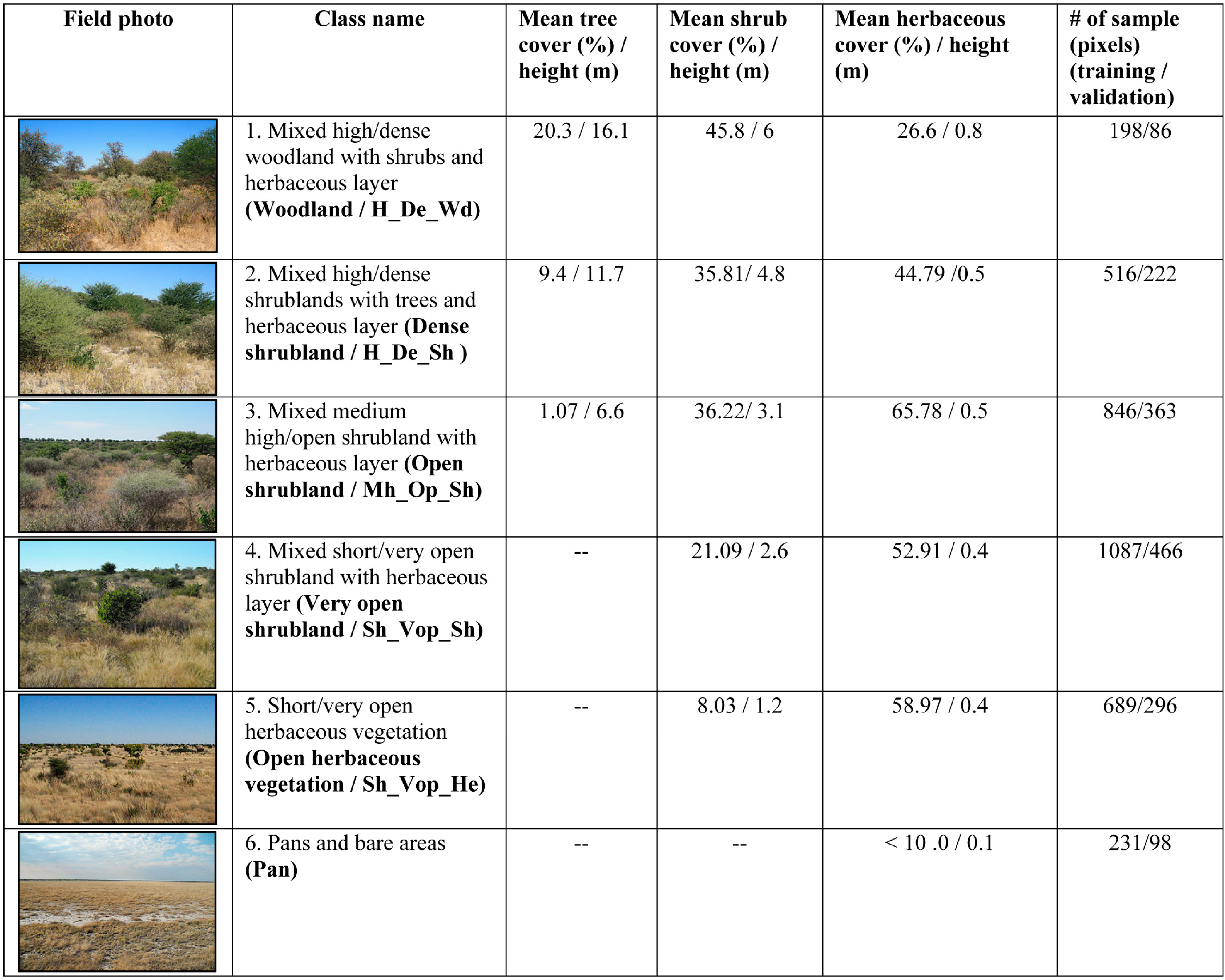
3.1. Field Data Processing and Development of Vegetation Morphology Class

Filed data related to vegetation physiognomy (i.e., structure and density) and species composition were acquired following a transect-based approach during two field campaigns conducted during 18 May–12 June 2011 and 9–29 May 2012. Transect locations were based on knowledge gained during May 2010 reconnaissance trip and visual interpretation of high spatial resolution imagery (i.e., GeoEye/SPOT) with the objective to sample all important vegetation morphology types in the study area. An important factor for selecting the location of field transects was the morphological homogeneity of the sample location up to the extent of 2 × 2 MOD13Q1 pixels (i.e., 0.22 km2). Besides visually interpreting the high spatial resolution imagery, this step was also aided by the homogeneous image objects generated from multi-resolution segmentation of a Landsat TM imagery [22,44]. Nevertheless, due to accessibility and safety issues (e.g., danger of predator attack), these transects could not be established away from tracks except in the pan and more open areas. Combining the fieldwork conducted during 2011 and 2012, data were collected in 148 transects (Figure 1c). In each of these 30-m transects, geographic coordinates were recorded at the start and end points and a wooden pole with marked height was utilized to record the height of trees and shrubs and derive minimum, maximum and average woody vegetation height. Furthermore, the percent cover of trees, shrubs and grass cover was visually interpreted by two interpreters and records were tallied to estimate total tree, shrub and grass cover within each transect. These characteristics were also visually interpreted and recorded at 352 additional locations where setting up a transect was not possible due to high vegetation density and safety issues (Figure 1c).
In southern African savanna systems, at the low spatial/spectral resolution, vegetation physiognomic-structural aspects are the most important determinants of a pixels reflectance, rather than floristic properties [45]. To account for that vegetation morphology classes were developed based on (i) vegetation physiognomy (ii) vertical and horizontal agreement and (iii) leaf type. The accurate representation of the typical co-existence of tree, shrubs and grasses in savanna ecosystem requires consideration of the layering system of vegetation structure. An important advantage of considering the layering system in heterogeneous systems such as savannas is the independence of geographic scale [46]. Thus, considering the layering system of vegetation and above mentioned vegetation properties recorded in field transects, the following six vegetation morphology classes were defined: (i) Mixed high/dense woodland with shrubs and herbaceous layer (Woodland); (ii)Mixed high/dense shrublands with trees and herbaceous layer (Dense shrubland); (iii) Mixed medium high/open shrubland with herbaceous layer (Open shrubland); (iv) Mixed short/very open shrubland with herbaceous layer (Very open shrubland); (v) Short/open herbaceous vegetation (Grassland) and (vi) Pans and bare areas (Pan) (Figure 2).
Figure 2. Different vegetation morphology types and their physiognomic characteristics considered in this study as derived from field measurements.
Land 04 00197 g002

3.2. Remotely Sensed Data and Pre-Processing

The study used MODIS MOD13Q1 16-day composite 250-m NDVI product (Collection 5) which was acquired from NASA. The product was developed from atmospherically corrected bi-directional surface reflectance and had been masked for water, clouds, heavy aerosols and cloud shadows [47]. The study area was within a single MODIS tile no h20v11 and 14-years of NDVI data were utilized from scenes of 12 July 2000 (doy 193) to 26 June 2014 (doy 177) resulting in a total of 322 NDVI images.
An important issue with MODIS NDVI time-series is the presence of noise that can significantly impact quality of final output and thus needs to be carefully removed before analysis. To de-noise the NDVI time-series, the Savitzky-Golay (SG) filtering procedure was applied. The SG filtering procedure performs local polynomial regression to determine the smoothed data value at each data point and produces better results than adjacent averaging methods because it tends to preserve features of the original data, such as peak height and width. For this purpose, the MOD13 pixel reliability band was used to weight each data point in the time-series: value 0 (good data) had full weight (1), values 1–2 (marginal data) had half weight (0.5) and, value 3 (cloudy) had minimal weight (0.1). The SG function fitting was conducted within TIMESAT software [48] and parameters used included: number of envelope iterations 2, 4- and 5- point window over 2 fitting steps.

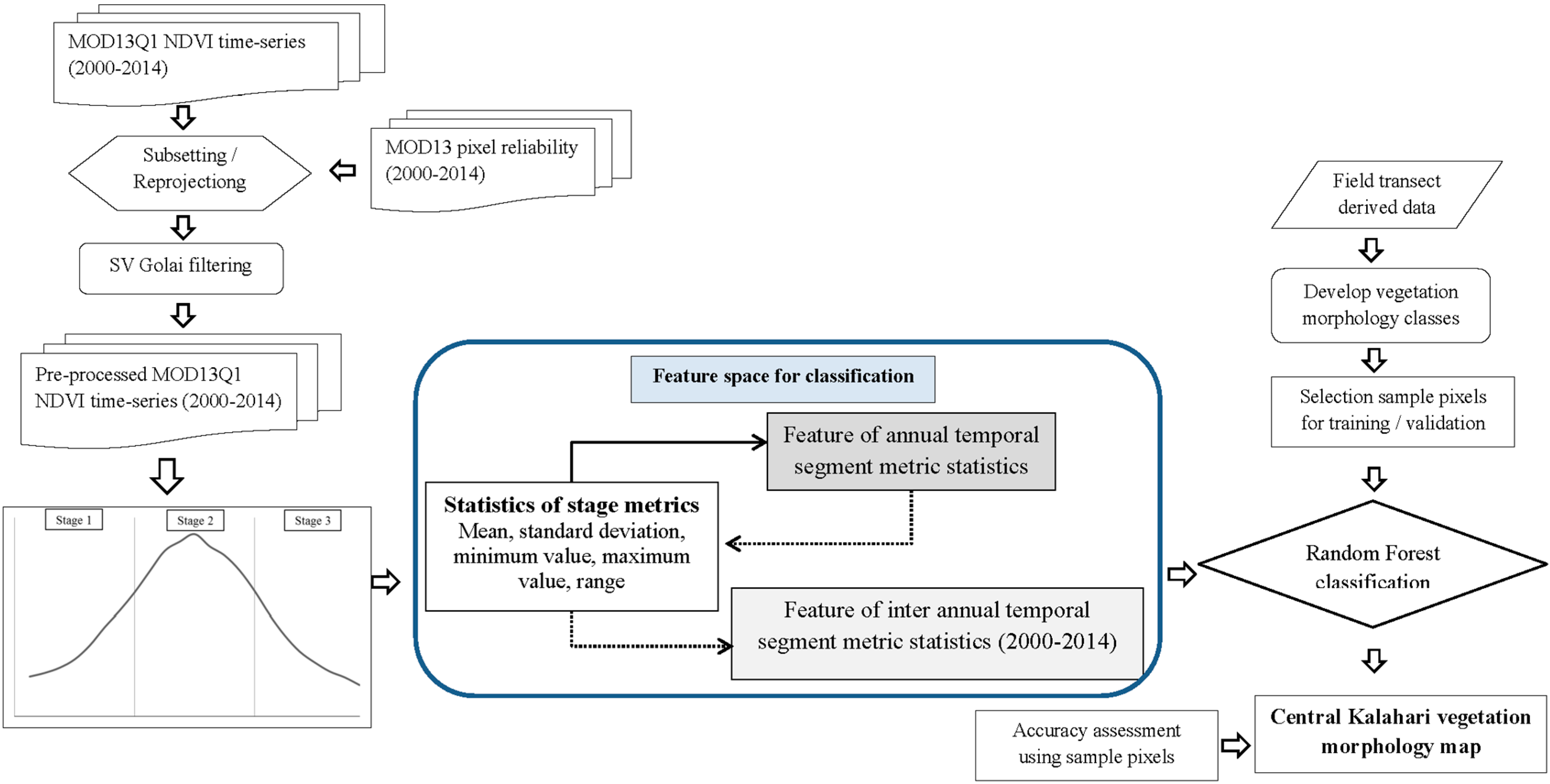
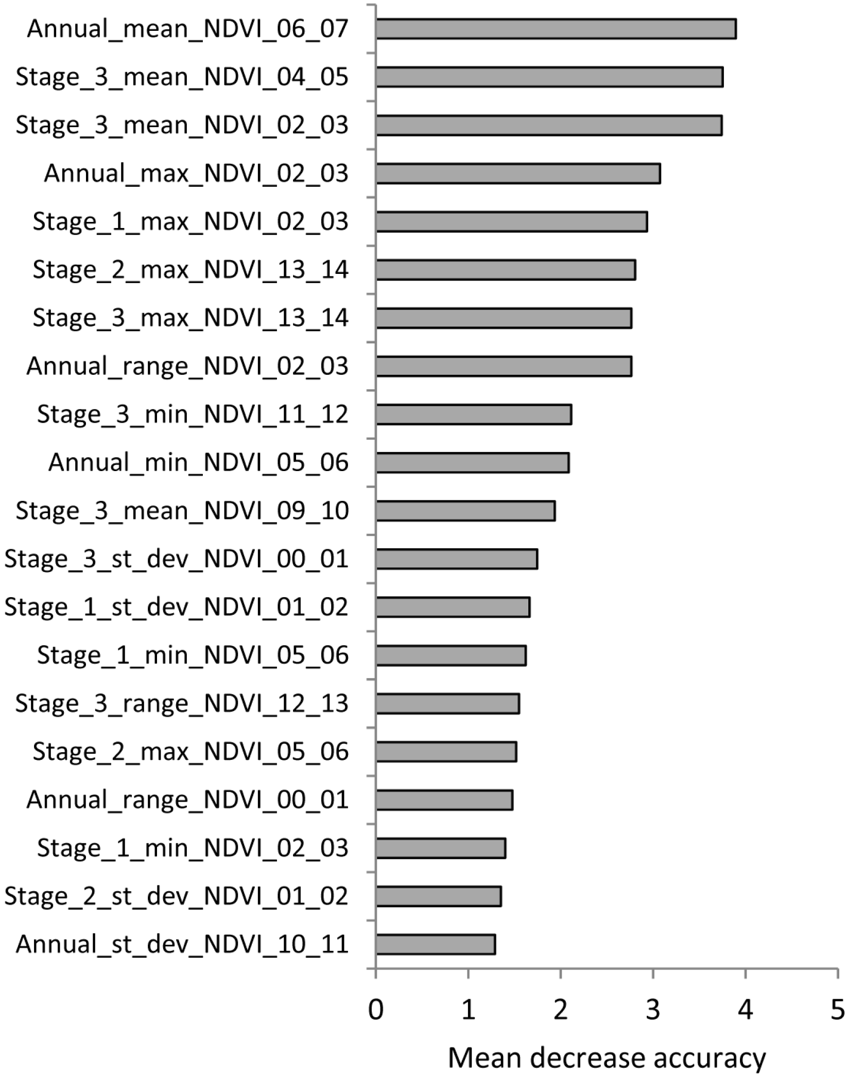
3.3. Calculating Time-Series Metrics, Separability Analysis and Random Forest Classification

Processed NDVI time-series data was utilized to derive annual and inter-annual statistical matrices (mean, standard deviation, minimum, maximum and range of NDVI). These matrices were first calculated for each of the 14-years. Furthermore, three temporal stages were defined from the NDVI time-series following the main seasonal characteristics of vegetation activity in the central Kalahari: first stage (December-March) represented the rainy season, stage two (April-July) the fall and winter season and third stage (August-November) spring and early summer. Generated feature space for final classification included 70 annual and 210 intra-annual features derived from the time-series NDVI (Figure 3).
Figure 3. Flowchart illustrating the methodology followed for mapping vegetation morphology types by combining field data with MODIS time-series derived matrices.
Land 04 00197 g003
Pixels for training the classifier and assessing the classification accuracy were selected based on: (i) spatial overlap with each field transect; and (ii) more pixels in the neighborhood of field transect locations were selected as samples by interpreting and confirming their homogeneity in terms of vegetation physiognomy by overlying them on high resolution imagery (GeoEye/SPOT). Since the high spatial resolution imagery (i.e., 11 SPOT tiles at 2.5 m spatial resolution) covered only 24% of the study area, more sample pixels were selected by carefully interpreting multi date high spatial resolution imagery available in Google Earth based on field knowledge. The use of Google Earth not only increased the number of samples but also improved its spatial distribution to cover off-track areas that were logistically challenging to cover during field work. 70% of the selected pixels were used for training the classifier and the remaining 30 percent were used for post-classification accuracy assessment (Figure 2). Spectral separability analysis was conducted to assess the separability of sample pixels of each vegetation morphology class using Jeffreys-Matusita distance (JM-distance) which is a pair-wise measure of class separability based on the probability distribution of two classes. JM-distance has a finite dynamic range that allows easier comparison of class separability [49].
Vegetation morphology types were mapped using an ensemble tree-based classifier called Random Forest (RF). The RF classifier builds multiple decision trees by bootstrapping samples of the reference data. Decision tree classifiers have advantages over traditional classifiers in that they make no assumptions about data distribution (e.g., normality) and can adapt to non-linear relationships inherent in the data [50]. In RF classification, each decision tree uses a random subset of training data and a random subset of input predictor variables which reduces the correlation between decision trees as well as the overall computational complexity. Roughly two thirds of the data is sampled with replacement while one third of the sample data is withheld from tree construction (also called “out-of-the-bag” or OOB samples). OOB samples are used to calculate the difference between predicted versus observed samples [51]. RF classification was implemented in the statistical package R using the “randomforest” package [52]. The parameters used for classification included: number of trees (ntree = 500), minimum samples in terminal node (nodesize = 10) and sqrt(p) as the number of variables randomly sampled as candidates at each split, where p is the number of variables. The classification accuracy was assessed using independent pixels reserved for each class. Accuracy was reported based on class-wise user’s and producer’s accuracy, overall accuracy and kappa statistic.

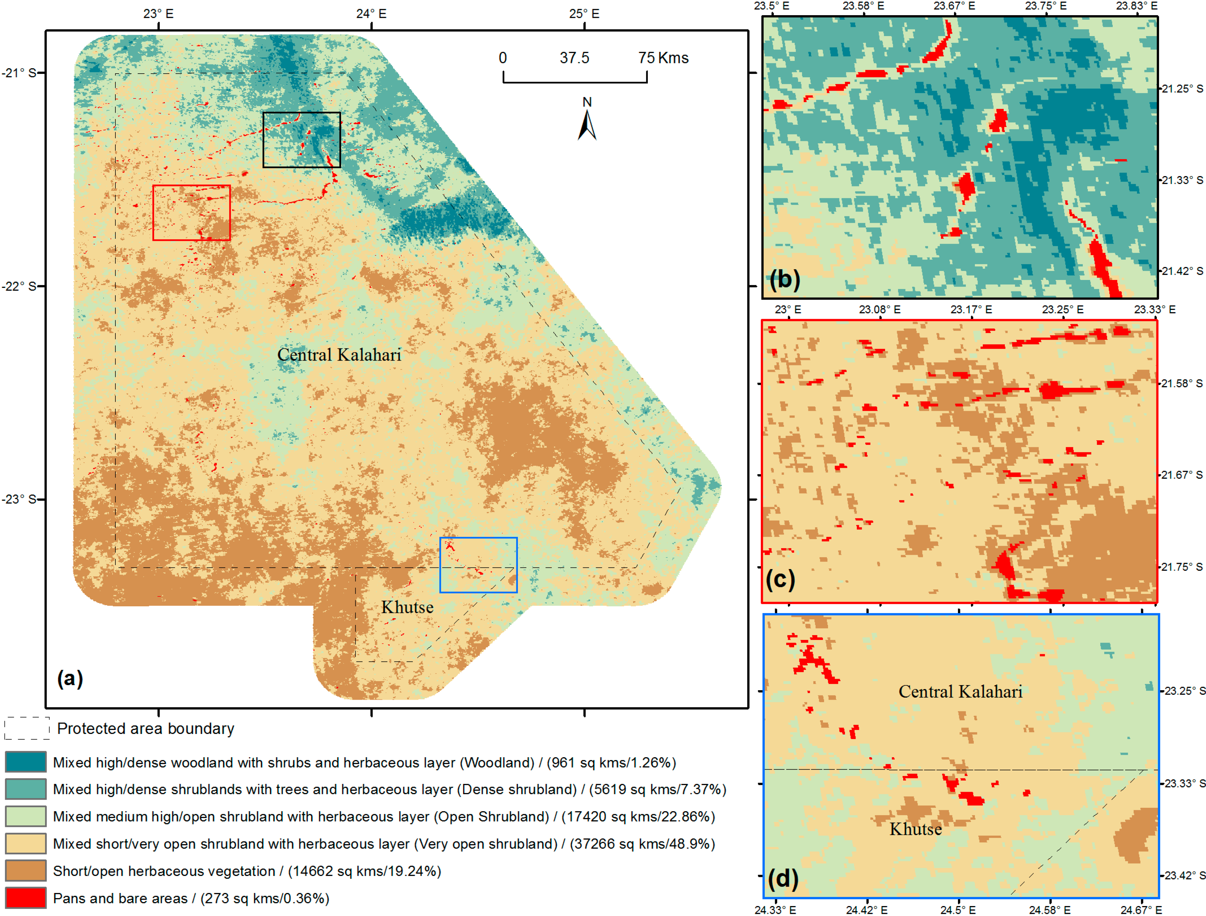
4. Results and Discussion

The characteristic phenological pattern of selected representative pixels of each vegetation morphology type is depicted by its NDVI time-series for the year 2010–2011 in Figure 4. Differences in the NDVI amplitude of various vegetation morphology classes are apparent especially during the peak of greenness and considering mean and range of NDVI values. In general, woodland areas (Figure 4i) have the highest mean annual NDVI and low standard deviation due to significant woody cover. As the woody cover density progressively decreases among different vegetation morphology types (e.g., open shrubland, very open shrubland), the peak of NDVI amplitude decreases along with increasing standard deviation of annual NDVI (due to the increasing contribution of herbaceous cover with temporally variable phenological response). Furthermore, pan areas show most distinct phenological pattern characterized by lowest peak of NDVI amplitude coupled with significant low range of NDVI. Differences are also visible in the green up and senescence between different vegetation morphology types due to the significantly steep onset on greenness for herbaceous dominated vegetated morphology types compared to slower onset in woody dominated vegetation morphology areas. Table 1 shows the JM-distance values calculated between samples of six vegetation morphology classes based on the NDVI time-series matrices. These results of separability analysis show high overall spectral separability among different vegetation morphology types (Table 1). Pan and bare areas had the highest spectral separability with all other vegetation morphology types, while H_De_Wd (i.e., class 1) and H_De_Sh (i.e., class 2) showed slightly lower separability value due to their structural and functional similarity.
Figure 4. NDVI temporal profiles of samples of each vegetation morphology type showing differences in NDVI magnitude and phenological properties for the year 2010–2011.
Land 04 00197 g004
Table 1. Spectral separability between different vegetation morphology classes reported as Jeffreys-Matusita (JM)-distance.
H_De_Wd (Woodland)H_De_Sh (Dense Shrubland)Mh_Op_Sh (Open Shrubland)Sh_Vop_Sh (Very Open Shrubland)Sh_Vop_He (Very Open Herbaceous Vegetation)Pans
H_De_Wd (Woodland)--1.881.911.991.991.99
H_De_Sh (Dense shrubland) --1.861.881.991.99
Mh_Op_Sh (Open shrubland) --1.911.951.99
Sh_Vop_Sh (Very open shrubland) --1.921.99
Sh_Vop_He (Very open herbaceous vegetation) --1.96
Pans --
The vegetation morphology type mapping in this study was based on in situ vegetation properties obtained during two field campaigns in the Central Kalahari. In general, vegetation in the study area represents a transition zone between tree savanna with mixed broad leaf and microphyllous (fine leafed) species in the northern and central part that gradually changes into microphyllous species dominated areas in the south and south-west. The mapped vegetation types for the whole study area is shown in Figure 5a which also shows areas with different dominant vegetation morphology types in inset figures. Results show that vegetation morphology class 4 (i.e., Mh_Op_Sh) was the spatially most dominant (covering about 48% area), whereas vegetation morphology class 6 (i.e., pans and bare areas) was least dominant (less than 1% area).Vegetation morphology classes 1, 2, 3, and 5 covered 1.26%, 7.37%, 22.86% and 19.24% of the study area respectively. Classification accuracy assessment using sample pixels showed an overall accuracy of 91.9% and kappa coefficient of 0.88 (Table 2). Highest individual class accuracy was achieved for pans and bare areas (i.e., producer’s accuracy 95.91%). The spatial distribution of the different vegetation morphology types in the study area is a reflection of the spatio-temporal variability in the ecological mechanisms (e.g., soil characteristics, rainfall pattern, fire history) that influence savanna vegetation structure and composition. Vegetation morphology class 1 was more common in the northern parts of the study area (Figure 5a). H_De_Wd and H_De_Sh are also noticeably present in the extreme north-western part, and are associated with the Ghanzi ridge marked by pre-Kalahari bedrock and shallow sand cover. During the field campaign, it was noted that the patches of H_De_Wd and H_De_Sh in the north and north-western part of study area were dominated by Terminalia prunioides mixed with Croton gratissimus and Acacia erioloba. In contrast, those in the north-eastern part were dominated by Colophospermum mopane, co-dominant Lonchocarpus nelsii and Acacia luederitzii. Most common woody species under Mh_Op_Sh and Sh_Vop_Sh areas were Lonchocarpus nelssi, Bauhinia petersiana, Grewia flava and Catophractes alexandri.
H_De_Wd and H_De_Sh generally dominate areas known as northern Kalahari sandveld that are topographically characterized by immobile longitudinal sand dunes. Mh_Op_Sh and Sh_Vop_Sh dominate areas that are topographically characterized as inter-dunal and plains with relatively shallow depth of sand. It also marks the transition zone between relatively densely vegetated areas and more open areas with predominantly herbaceous vegetation. Areas under Sh_Vop_He are mostly plains characterized by a top layer consisting of shallow sand. Dominant herbaceous species in the Sh_Vop_He area were Stipagrostis spp, Aristida spp. Pan areas have dominant clay content and are found in the study area as either ancient fossil river valley systems or others that are randomly scattered throughout the study area. Pan areas are characterized by occasional occurrence of clumps of trees also called “tree islands”, a result of the complex interaction of longer water availability, fire history and soil characteristics.
Figure 5. Vegetation morphology map of the central Kalahari produced as a result of this study.
Land 04 00197 g005
Table 2. Classification accuracy assessment based on independent samples for each class.
Class NameH_De_Wd (Woodland)H_De_Sh (Dense Shrubland)Mh_Op_Sh (Open Shrubland)Sh_Vop_Sh (Very Open Shrubland)Sh_Vop_He (Very Open Herbaceous Vegetation)PansProducer’s Accuracy (%)
H_De_Wd (Woodland)7943---91.86
H_De_Sh (Dense shrubland)1420152--90.54
Mh_Op_Sh (Open shrubland)114336102-92.56
Sh_Vop_Sh (Very open shrubland)-22104295-92.06
Sh_Vop_He (Very open herbaceous vegetation)--817268390.54
Pans----39495.91
User’s accuracy (%)84.0483.492.8193.6695.3796.9
Overall accuracy: 91.96%; Kappa: 0.88.
With the possibility of generating hundreds of features using time-series remotely sensed imagery, analysis could be very time consuming and/or computationally intensive. Variable importance based pre-selection of most important time-series metrics can address this issue and also provide an insight into the ecological meaning of selected metrics. Figure 6 shows the 20 most overall important variables in order of decreasing importance used for mapping vegetation types in the central Kalahari savanna. Annual mean NDVI (2006–2007) was the most important feature, underscoring the distinguishability of vegetation morphology types in dry savannas based on their overall annual productivity. Furthermore, 14 out of the 20 most important variables (and 6 out of the top 10 variables) were intra-annual metrics representing some characteristic of the vegetation greenness during one of the three considered stages. These results highlight that annual vegetation productivity matrices may have too low information content for distinguishing semi-arid savanna vegetation types as some vegetation morphology types may have similar mean annual NDVI intensity. Distinguishing vegetation morphology types in dry savanna characterized by low niche differentiation require intensity metrics derived from various phenological stages. Furthermore, it is also important to notice that these most significant variables are from various years of the 14-years study period, suggesting to the suitability of longer length of satellite time-series for distinguishing savanna vegetation types.
Previous studies in African savannas have established that several factors including fire history, rainfall pattern, grazing pressure leads to changes in savanna vegetation’s structural configuration over time [53,54]. In particular, vegetation conditions in semi-arid savannas are sensitive to short term rainfall variability [18,55]. Considering these factors and the fact that in situ data for this study were acquired during 2011 and 2012 (combined with high spatial resolution imagery whenever available), a limitation of the produced vegetation morphology map is that it is more representative of post-2010 spatial distribution of vegetation morphology types in the central Kalahari. Although the 14-years of NDVI time-series was utilized, the resultant mapping output may not represent the spatial distribution of vegetation morphology types with the same accuracy as reported. However it should also be considered that classes with significant woody vegetation and/or pan areas may considerably accurately represent the past distributions as the impacts of memory effects is less significant in woody dominated vegetation types (compared to herbaceous dominate areas) as they are more resilient to environmental variability [56]. The motivation for utilizing NDVI time-series over the 14-year period, as carried out in this study, was to provide suitable dimensionality of predictor variables that could be needed for spectrally distinguish the vegetation types. Metrics derived from such a longer time-series allowed to account for the confounding effects of inter-annual variability (in response to changing rainfall and/or fire) and provided a realistic overall distribution of vegetation morphology types in a characteristically non-equilibrium dryland savanna ecosystem.
Figure 6. Variable importance plot of 20 most significant variables reported as mean decrease in overall accuracy determined during the OOB error calculation in random forest classification. Variables with large decrease in accuracy are considered more important for classification.
Land 04 00197 g006
Furthermore, while MODIS time-series utilized in this study provides the best compromise considering spatial resolution, swath area and temporal resolution, it may not be able to suitably represent the fine-scale spatial heterogeneity observed in savanna landscapes due to low spatial resolution (i.e., 232 m). Although higher spatial resolution data (e.g., Landsat, SPOT) can account for this spatial heterogeneity but poses challenges such as: (i) the study area is spread across 6 Landsat tiles leading to issues of unavailability of temporally consistent and comparable cloud free scenes; and (ii) the requirement of computational power and memory related issues due to much larger size of higher spatial resolution time-series. To overcome the limitation of hard classifiers and to more accurately represent the landscape heterogeneity, recent studies have also adopted fractional cover based approach using higher spatial resolution data [57,58]. However, adopting a fractional cover based approach deemed unsuitable for this study because it very difficult to find meaningful and representative endmembers for the considered vegetation morphology classes at the spatial resolution of a MODIS pixel. Also, at lower spatial resolution (e.g., MODIS) sub-pixel abundance estimates in savannas are more closely associated with the functional properties of vegetation (e.g., photosynthetic versus non-photosynthetic) rather than structural properties [59].
The comparison of the GlobCover product with the vegetation morphology map produced in this study shows some of the limitations of LCCS legend based map which may be suitable/consistent for global scale applications but produces oversimplified/generalized representation of landscape structural heterogeneity and functional diversity at landscape to regional scales. In the study area while the GlobCover product showed more than 90% area as a single land cover type, the results of this study showed less than 50% of the study area within a single class. Additionally, the use of in situ data captures the spatial variability in vegetation structural properties which is suitably represented in the vegetation morphology map produced in this study.

5. Summary

This study highlights the importance of combining in situ data with satellite derived time-series matrices of vegetation greenness for distinguishing and accurately mapping vegetation morphology types in a dry savanna that are challenging to separate due to low niche differentiation in spatial domain. A significant impediment for ecological research in southern Africa savanna in general, and the central Kalahari in particular, is the lack of basic geospatial data on vegetation types, land cover properties that is critical for accessing human impacts, as well as influence of climatic variability leading to effective biodiversity conservation and management. The vegetation morphology map produced in this study is the first such product for this geographically extensive area and is being provided to our collaborators and other researchers working in central Kalahari (including the officials in the Department of Wildlife and National Parks of Botswana Government). We hope that this vegetation morphology map will serve as a valuable input for understanding spatio-temporal patterns of habitat use by both predator and prey species in the central Kalahari. By analyzing wildlife movement data collected using GPS collars in association with the vegetation morphology map, researchers will be able to identify how spatio-temporal patterns in their movement are associated with landscape properties in both the dry and wet seasons. More specifically, basic spatial analysis using vegetation morphology map and wildlife movement data could identify areas where predators are digging holes across game fences to leave the protected area in search of easy livestock prey, resulting in human–wildlife conflict. Furthermore, the vegetation morphology map could be used in conjunction with either in situ or satellite derived fire history to develop understanding of the fire susceptibility and fire return interval properties of different vegetation types. Overall these analyses would enable researchers in developing enhanced understanding of the ecological functioning, pattern of habitat use by the wildlife, effectiveness and suitability of game fencing, and eventually resulting in ecologically informed decision-making and sustainable ecosystem management in the central Kalahari. Still much larger areas in Botswana are unmapped/unexplored in terms of vegetation structural properties and/or floristic composition. The greatest challenge for expanding the satellite based vegetation morphology type mapping to other parts of Botswana is the lack of in situ data of vegetation properties. Our experience in the central Kalahari suggests that careful visual interpretation of high spatial resolution (<5 m) imagery can substitute field data to a certain extent and needs to be utilized in combination with coarser spatial resolution imagery for characterizing savanna vegetation properties in other understudied areas within southern Africa.

Acknowledgments

This study was supported by National Science Foundation: Doctoral Dissertation Research Improvement Grant # 1203580 and Veselka Field Research Grant from University of Texas. High spatial resolution imagery were provided as multiple imagery grants from the GeoEye Foundation and Planet Action (AUSTRIM). The authors would like to thank Glyn Maude for logistical support; Kevin MacFarlane, Moses Selebasto and field assistants for help during field campaigns in the central Kalahari. The authors also thank Lars Eklundh for suggestions regarding data pre-processing and the two anonymous reviewers for their insightful comments.

Author Contributions

Niti Mishra collected field data, conducted data analysis and led the preparation of the manuscript with conceptual inputs from Kelley Crews, Jennifer Miller and Thoralf Meyer. Thoralf Meyer and Jennifer Miller also helped in structuring and editing the manuscript.

Conflicts of Interest

The authors declare no conflict of interest.

References

  1. Balmford, A.; Moore, J.L.; Brooks, T.; Burgess, N.; Hansen, L.A.; Williams, P.; Rahbek, C. Conservation conflicts across africa. Science 2001, 291, 2616–2619. [Google Scholar] [CrossRef] [PubMed]
  2. Von Richter, W. The status of wildlife conservation in botswana. Koedoe 2014, 20, 143. [Google Scholar]
  3. Thomas, D.S.G.; Twyman, C. Good or bad rangeland? Hybrid knowledge, science, and local understandings of vegetation dynamics in the Kalahari. Land Degrad. Dev. 2004, 15, 215–231. [Google Scholar] [CrossRef]
  4. Winterbach, H.E.; Winterbach, C.W.; Somers, M.J. Landscape suitability in botswana for the conservation of its six large African carnivores. PLoS One 2014, 9, e100202. [Google Scholar] [CrossRef] [PubMed]
  5. Dougill, A.J.; Thomas, D.S.G.; Heathwaite, A.L. Environmental change in the kalahari: Integrated land degradation studies for nonequilibrium dryland environments. Ann. Assoc. Am. Geog. 1999, 89, 420–442. [Google Scholar] [CrossRef]
  6. Ferguson, K.; Hanks, J. The effects of protected area and veterinary fencing on wildlife conservation in southern Africa. PARKS 2012, 18, 49. [Google Scholar]
  7. Deaprtment of Wildlife and National Park (DWNP), Government of Botswana. Central Kalahari and Kutse Game Reserve Management Plan; DWNP: Gaborone, Botswana, 2003.
  8. Kesch, K.M.; Bauer, D.T.; Loveridge, A.J. Undermining game fences: Who is digging holes in Kalahari sands? Afr. J. Ecol. 2014, 52, 144–150. [Google Scholar] [CrossRef]
  9. Vanderpost, C.; Ringrose, S.; Matheson, W.; Arntzen, J. Satellite based long-term assessment of rangeland condition in semi-arid areas: An example from Botswana. J. Arid Environ. 2011, 75, 383–389. [Google Scholar] [CrossRef]
  10. Ringrose, S.; Matheson, W.; Wolski, P.; Huntsman-Mapila, P. Vegetation cover trends along the Botswana Kalahari transect. J. Arid Environ. 2003, 54, 297–317. [Google Scholar] [CrossRef]
  11. Moleele, N.; Ringrose, S.; Matheson, W.; Vanderpost, C. More woody plants? The status of bush encroachment in Botswana’S grazing areas. J. Environ. Manag. 2002, 64, 3–11. [Google Scholar] [CrossRef]
  12. Solomon, S.D.; Qin, M.; Manning, Z.; Chen, M.; Marquis, K.B.; Averyt, M.; Tignor, H.L. Climate Change: The Physical Science Basis, Contribution of Working Group I to the Fourth Assessment Report of the Intergovernmental Panel on Climate Change; Cambridge Univeristy Press: Cambridge, UK, 2007. [Google Scholar]
  13. Thomas, D.S.G.; Knight, M.; Wiggs, G.F.S. Remobilization of southern African desert dune systems by Twenty-First Century global warming. Nature 2005, 435, 1218–1221. [Google Scholar] [CrossRef] [PubMed]
  14. Scholes, R.J.; Walker, B.H. Cambridge Studies in Applied Ecology and Resource Management—An African Savanna: Synthesis of the Nylsvley Study; Cambridge University Press: Cambridge, UK, 1993. [Google Scholar]
  15. Van Rooyen, N.; Bezuidenhout, D.; Theron, G.K.; Bothma, J.D.P. Monitoring of the vegetation around artificial watering points (windmills) in the Kalahari Gemsbok National Park. Koedoe 1990, 33, 63–88. [Google Scholar] [CrossRef]
  16. Loarie, S.R.; Tambling, C.J.; Asner, G.P. Lion hunting behaviour and vegetation structure in an African savanna. Anim. Behav. 2013, 85, 899–906. [Google Scholar] [CrossRef]
  17. Pettorelli, N.; Laurance, W.F.; O’Brien, T.G.; Wegmann, M.; Nagendra, H.; Turner, W. Satellite remote sensing for applied ecologists: Opportunities and challenges. J. Appl. Ecol. 2014, 51, 839–848. [Google Scholar] [CrossRef]
  18. Huttich, C.; Gessner, U.; Herold, M.; Strohbach, B.J.; Schmidt, M.; Keil, M.; Dech, S. On the suitability of MODIS time series metrics to map vegetation types in dry savanna ecosystems: A case study in the Kalahari of Ne Namibia. Remote Sens. 2009, 1, 620–643. [Google Scholar] [CrossRef]
  19. Thomas, D.S.G. Sand, grass, thorns, and ... cattle: The modern Kalahari environment. In Sustainable Livelihoods in Kalahari. Environments: Contributions to Global Debates; Sporton, D., Thomas, D.S.G., Eds.; Oxford University Press: Oxford, UK, 2002; pp. 39–66. [Google Scholar]
  20. Mishra, N.B. Characterizing Ecosystem Structural and Functional Properties in the Central Kalahari Using Multi-Scale Remote Sensing. Docter’s Thesis, University of Texas, Austin, TX, USA, 2014. [Google Scholar]
  21. Ringrose, S.; Jellema, A.; Huntsman-Mapila, P.; Baker, L.; Brubaker, K. Use of remotely sensed data in the analysis of soil-vegetation changes along a drying gradient peripheral to the Okavango Delta, Botswana. Int. J. Remote Sens. 2005, 26, 4293–4319. [Google Scholar] [CrossRef]
  22. Mishra, N.B.; Crews, K.A. Mapping vegetation morphology types in a dry savanna ecosystem: Integrating hierarchical object-based image analysis with random forest. Int. J. Remote Sens. 2014, 35, 1175–1198. [Google Scholar] [CrossRef]
  23. Bontemps, S.; Defourny, P.; Bogaert, E.V.; Arino, O.; Kalogirou, V.; Perez, J.R. Globcover 2009-Products Description and Validation Report. 2011. Available online: http://dup.esrin.esa.int/files/p68/GLOBCOVER2009_Validation_Report_2.2.pdf (accessed on 3 September 2014).
  24. Hill, M.J.; Román, M.O.; Schaaf, C.B. Dynamics of vegetation indices in tropical and subtropical savannas defined by ecoregions and moderate resolution imaging spectroradiometer (MODIS) land cover. Geocarto Int. 2012, 27, 153–191. [Google Scholar] [CrossRef]
  25. Wu, J.; Marceau, D. Modeling complex ecological systems: An introduction. Ecol. Model. 2002, 153, 1–6. [Google Scholar] [CrossRef]
  26. Elmore, A.J.; Mustard, J.F.; Manning, S.J.; Lobell, D.B. Quantifying vegetation change in semiarid environments: Precision and accuracy of spectral mixture analysis and the normalized difference vegetation index. Remote Sens. Environ. 2000, 73, 87–102. [Google Scholar] [CrossRef]
  27. Jensen, J.R. Remote Sensing of the Environment: An Earth Resource Perspective 2/e; Pearson Education India: Chennai, India, 2009. [Google Scholar]
  28. De Fries, R.; Hansen, M.; Townshend, J.; Sohlberg, R. Global land cover classifications at 8 km spatial resolution: The use of training data derived from Landsat imagery in decision tree classifiers. Int. J. Remote Sens. 1998, 19, 3141–3168. [Google Scholar] [CrossRef]
  29. Hansen, M.; DeFries, R.; Townshend, J.; Carroll, M.; Dimiceli, C.; Sohlberg, R. Global percent tree cover at a spatial resolution of 500 m: First results of the MODIS vegetation continuous fields algorithm. Earth Interact. 2003, 7, 1–15. [Google Scholar] [CrossRef]
  30. Jacquin, A.; Sheeren, D.; Lacombe, J.-P. Vegetation cover degradation assessment in madagascar savanna based on trend analysis of MODIS NDVI time series. Int. J. Appl. Earth Observ. Geoinf. 2010, 12, S3–S10. [Google Scholar] [CrossRef]
  31. Okin, G.S.; Roberts, D.A. Remote sensing in arid regions: Challenges and opportunities. In Manual of Remote Sensing—Volume 4, Remote Sensing for Natural Resource Management and Environmental Monitoring, 3rd ed.; Ustin, S., Ed.; John Wiley & Sons, Inc.: New York, NY, USA, 2004; pp. 111–146. [Google Scholar]
  32. Colditz, R.; Schmidt, M.; Conrad, C.; Hansen, M.; Dech, S. Land cover classification with coarse spatial resolution data to derive continuous and discrete maps for complex regions. Remote Sens. Environ. 2011, 115, 3264–3275. [Google Scholar] [CrossRef]
  33. Friedl, M.; Zhang, X.; Strahler, A. Characterizing global land cover type and seasonal land cover dynamics at moderate spatial resolution with MODIS data. In Land Remote Sensing and Global Environmental Change; Springer: Berlin, Germany, 2011; pp. 709–724. [Google Scholar]
  34. Clark, M.L.; Aide, T.M.; Grau, H.R.; Riner, G. A scalable approach to mapping annual land cover at 250 m using MODIS time series data: A case study in the dry chaco ecoregion of South America. Remote Sens. Environ. 2010, 114, 2816–2832. [Google Scholar] [CrossRef]
  35. Klein, I.; Gessner, U.; Kuenzer, C. Regional land cover mapping and change detection in central asia using MODIS time-series. Appl. Geogr. 2012, 35, 219–234. [Google Scholar] [CrossRef]
  36. Ghimire, B.; Rogan, J.; Galiano, V.R.; Panday, P.; Neeti, N. An evaluation of bagging, boosting, and random forests for land-cover classification in Cape Cod, Massachusetts, USA. GISci. Remote Sens. 2012, 49, 623–643. [Google Scholar] [CrossRef]
  37. Waske, B.; Benediktsson, J.A.; Sveinsson, J.R. Chapter 18 Random forest classification of remote sensing data. In Signal Image Processing for Remote Sensing; CRC Press: Boca Raton, FL, USA, 2012; pp. 365–374. [Google Scholar]
  38. Verikas, A.; Gelzinis, A.; Bacauskiene, M. Mining data with random forests: A survey and results of new tests. Pattern Recognit. 2011, 44, 330–349. [Google Scholar] [CrossRef]
  39. Mendelsohn, J.; El Obeid, S. Okavango River: The Flow of A Lifeline; Struik Publishers: Cape Town, South Africa, 2004. [Google Scholar]
  40. Scholes, R.J.; Dowty, P.R.; Caylor, K.; Parsons, D.A.B.; Frost, P.G.H.; Shugart, H.H. Trends in savanna structure and composition along an aridity gradient in the Kalahari. J. Veg. Sci. 2002, 13, 419–428. [Google Scholar] [CrossRef]
  41. Makhabu, S.W.; Marotsi, B.; Perkins, J. Vegetation gradients around artificial water points in the central Kalahari game reserve of Botswana. Afr. J. Ecol. 2002, 40, 103–109. [Google Scholar] [CrossRef]
  42. Thomas, D.S.G.; Shaw, P.A. The Kalahari Environment; Cambridge University Press: Cambridge, UK, 1991. [Google Scholar]
  43. Fagan, W.F. Connectivity, fragmentation, and extinction risk in dendritic metapopulations. Ecology 2002, 83, 3243–3249. [Google Scholar] [CrossRef]
  44. Mishra, N.B.; Crews, K.A. Estimating fractional land cover in semi-arid central kalahari: The impact of mapping method (spectral unmixing versus object based image analysis) and vegetation morphology. Geocarto Int. 2014, 29, 860–877. [Google Scholar] [CrossRef]
  45. Thompson, M. Standard land-cover classification scheme for remote-sensing applications in South Africa. South. Afr. J. Sci. 1996, 29, 36–42. [Google Scholar]
  46. Groffman, P.M.; Tiedje, T.M.; Mokma, D.L.; Simkins, S. Regional-scale analysis of denitrification in north temperate forest soils. Landsc. Ecol. 1992, 7, 45–53. [Google Scholar] [CrossRef]
  47. Huete, A.; Didan, K.; Miura, T.; Rodriguez, E.P.; Gao, X.; Ferreira, L.G. Overview of the radiometric and biophysical performance of the MODIS vegetation indices. Remote Sens. Environ. 2002, 83, 195–213. [Google Scholar] [CrossRef]
  48. Jonsson, P.; Eklundh, L. Timesat—A program for analyzing time-series of satellite sensor data. Comput. Geosci. 2004, 30, 833–845. [Google Scholar] [CrossRef]
  49. Laliberte, A.; Browning, D.; Rango, A. A comparison of three feature selection methods for object-based classification of sub-decimeter resolution UltraCam-l imagery. Int. J. Appl. Earth Observ. Geoinf. 2012, 15, 70–78. [Google Scholar] [CrossRef]
  50. Friedl, M.A.; Brodley, C.E. Decision tree classification of land cover from remotely sensed data. Remote Sens. Environ. 1997, 61, 399–409. [Google Scholar] [CrossRef]
  51. Breiman, L. Random forests. Mach. Learn. 2001, 45, 5–32. [Google Scholar] [CrossRef]
  52. Liaw, A.; Weiener, M. Classification and regression by randomforest. R News 2002, 2, 18–22. [Google Scholar]
  53. Levick, S.R.; Asner, G.P.; Kennedy-Bowdoin, T.; Knapp, D.E. The relative influence of fire and herbivory on savanna three-dimensional vegetation structure. Biol. Conserv. 2009, 142, 1693–1700. [Google Scholar] [CrossRef]
  54. Sankaran, M.; Ratnam, J.; Hanan, N. Woody cover in African savannas: The role of resources, fire and herbivory. Glob. Ecol. Biogeogr. 2008, 17, 236–245. [Google Scholar] [CrossRef]
  55. Vanacker, V.; Linderman, M.; Lupo, F.; Flasse, S.; Lambin, E. Impact of short-term rainfall fluctuation on interannual land cover change in Sub-Saharan Africa. Glob. Ecol. Biogeogr. 2005, 14, 123–135. [Google Scholar] [CrossRef]
  56. Archibald, S.; Scholes, R. Leaf green-up in a semi-arid African savanna-separating tree and grass responses to environmental cues. J. Veg. Sci. 2007, 18, 583–594. [Google Scholar]
  57. Gessner, U.; Machwitz, M.; Conrad, C.; Dech, S. Estimating the fractional cover of growth forms and bare surface in savannas. A multi-resolution approach based on regression tree ensembles. Remote Sens. Environ. 2013, 129, 90–102. [Google Scholar] [CrossRef] [Green Version]
  58. Mishra, N.B.; Crews, K.A.; Okin, G.S. Relating spatial patterns of fractional land cover to savanna vegetation morphology using multi-scale remote sensing in the central Kalahari. Int. J. Remote Sens. 2014, 35, 2082–2104. [Google Scholar] [CrossRef]
  59. Guerschman, J.P.; Hill, M.J.; Renzullo, L.J.; Barrett, D.J.; Marks, A.S.; Botha, E.J. Estimating fractional cover of photosynthetic vegetation, non-photosynthetic vegetation and bare soil in the Australian tropical savanna region upscaling the EO-1 hyperion and MODIS sensors. Remote Sens. Environ. 2009, 113, 928–945. [Google Scholar] [CrossRef]

