Spatially-Explicit Simulation of Urban Growth through Self-Adaptive Genetic Algorithm and Cellular Automata Modelling


Abstract
:1. Introduction
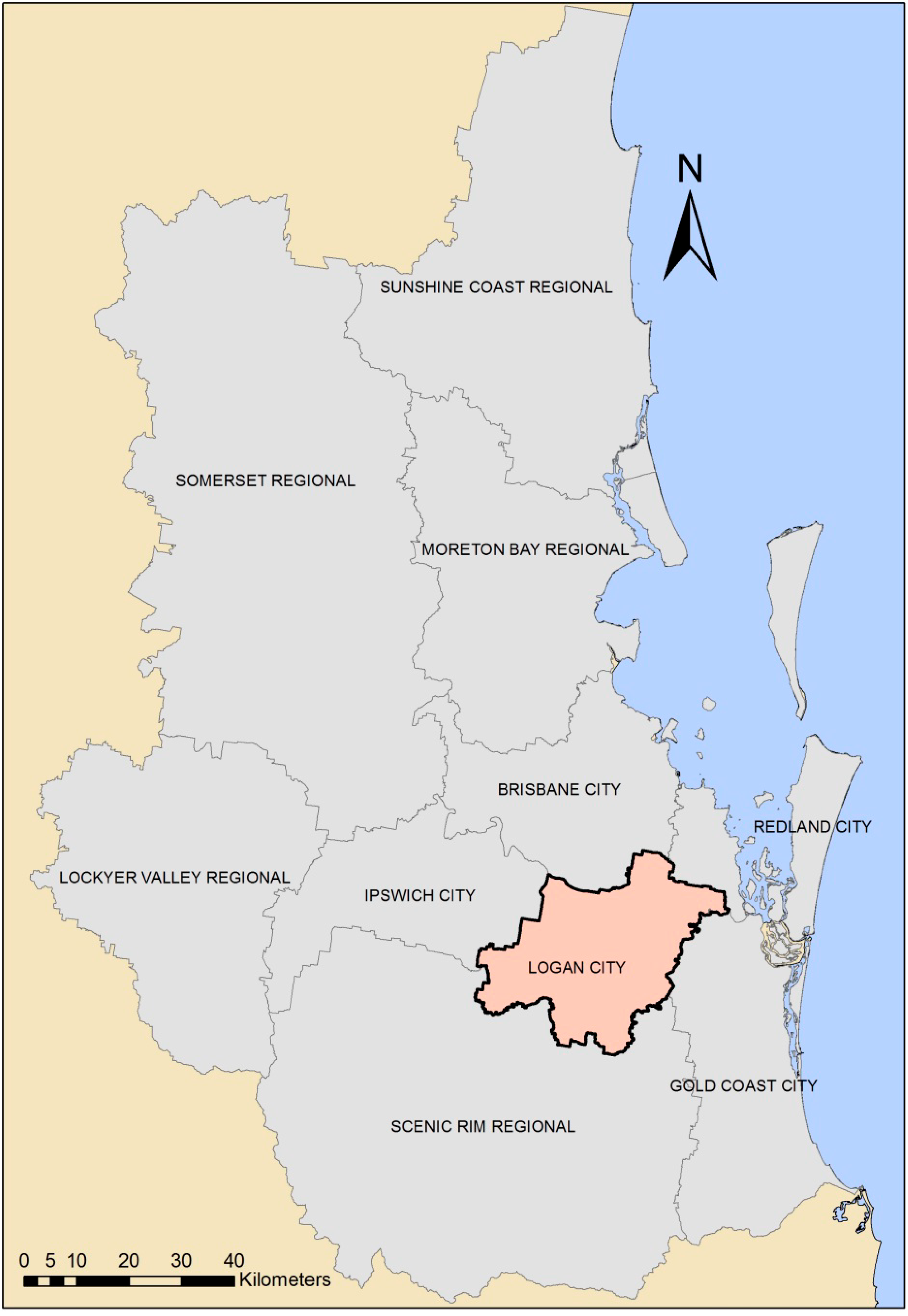
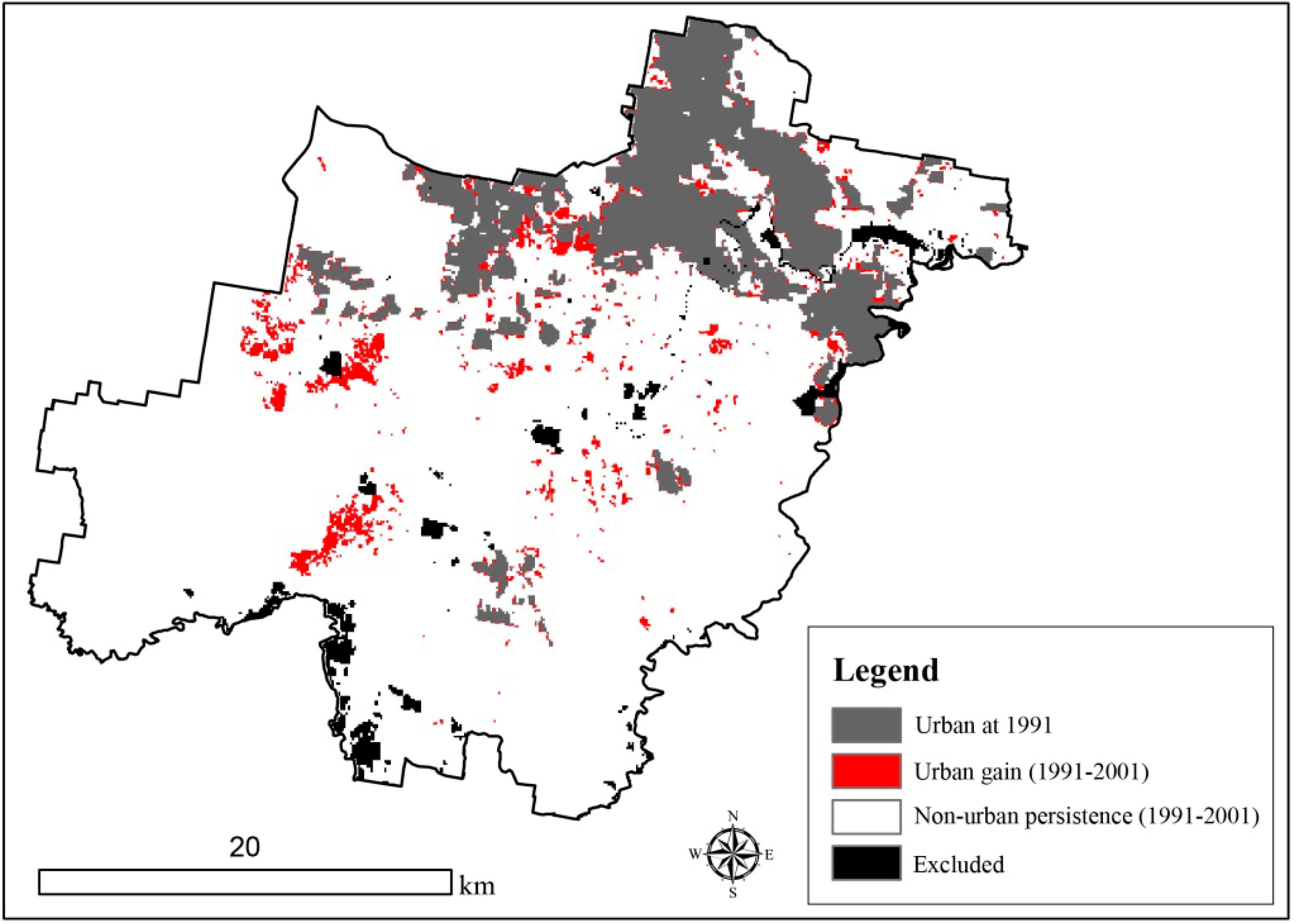
2. Study Area and Data


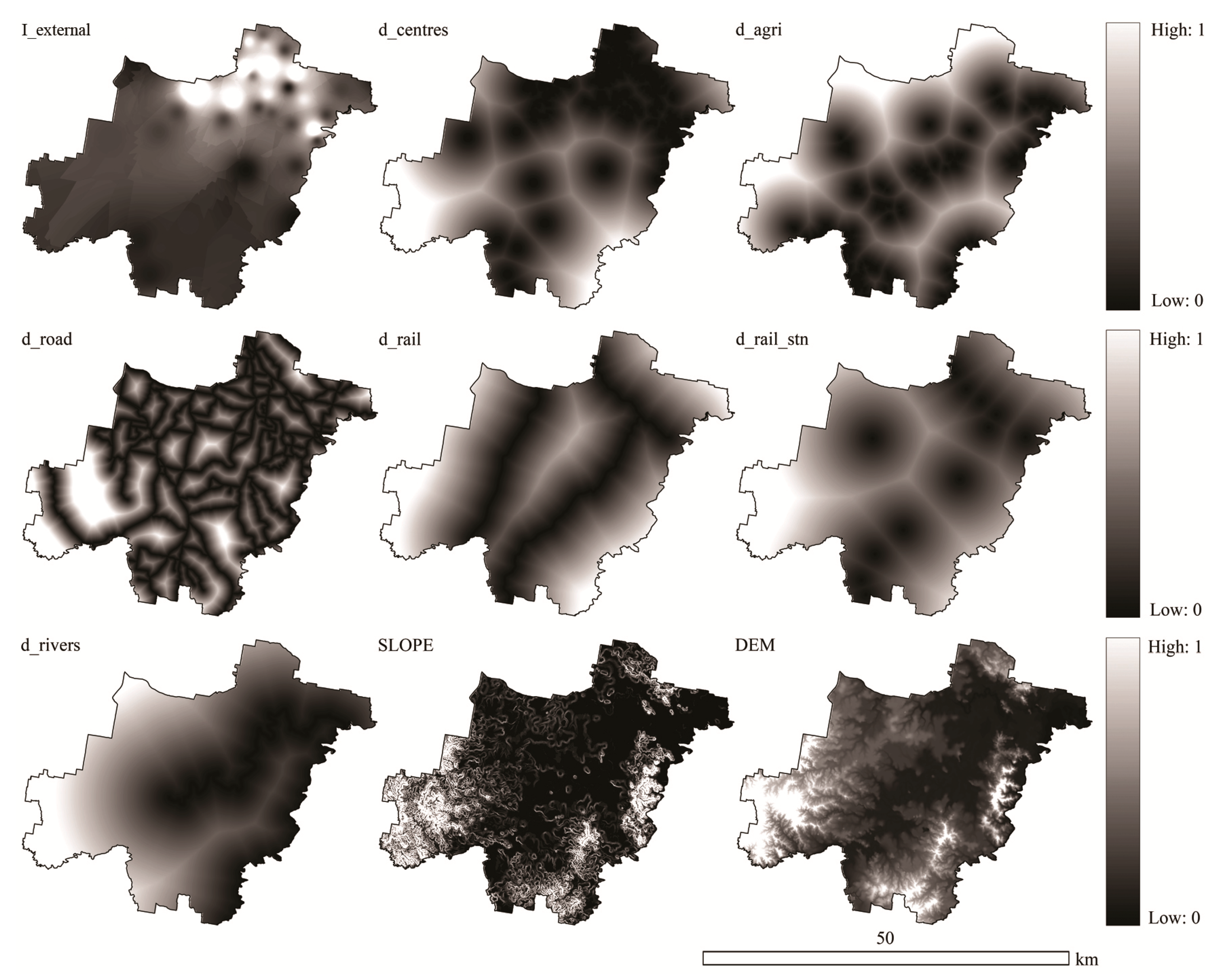
| Variable | Meaning | Data Extraction |
|---|---|---|
| I_external | Impact of urban centres surrounding Logan City (including Brisbane, Ipswich, Gold Coast and Redland cities) on the urban growth within the region | Calculated using Journey to Work data from Logan to the neighbouring regions from the 2006 Census |
| d_centres | Distance to urban centres within the region | Measured in GIS from the urban centres data layer |
| d_agri | Distance to agricultural land | Measured in GIS from the land use data layer |
| d_road | Distance to main roads | Measured in GIS from the transportation network data layer |
| d_rail | Distance to railway lines | |
| d_rail_stn | Distance to railway stations | |
| d_rivers | Distance to rivers | Measured in GIS from the land use data layer |
| SLOPE | Land slope | Extracted from the DEM |
| DEM | Land elevation | |
 | Probability of a cell changing its state from time t to the next time within a square 5 × 5-cell neighbourhood | Calculated using the focal function in GIS according to Equation (3) presented in Section 3.1 |
| R | Stochastic disturbance of unknown errors | Generated randomly using Equation (4) presented in Section 3.1 |
3. Method

3.1. Cellular Automata Model


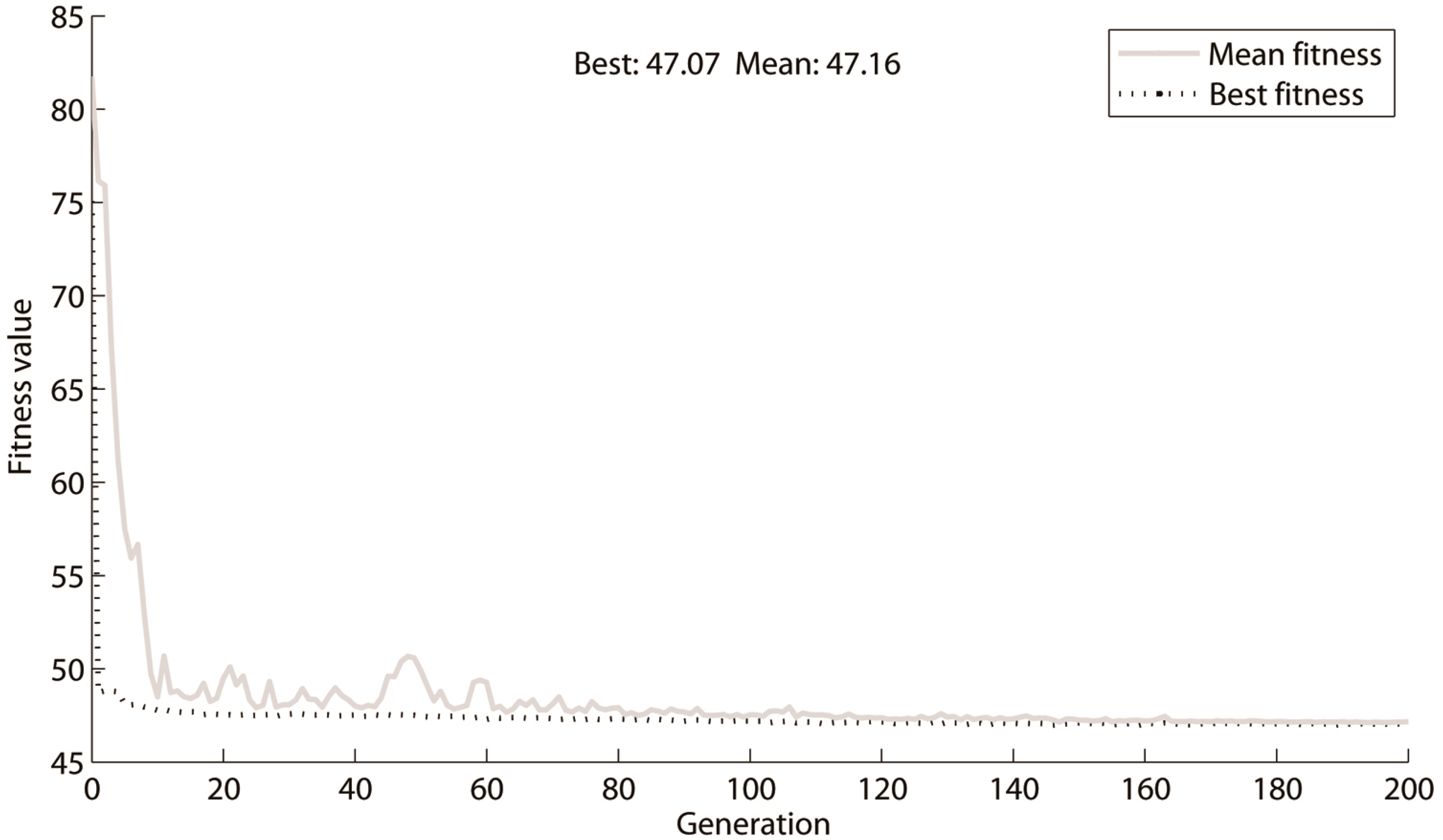
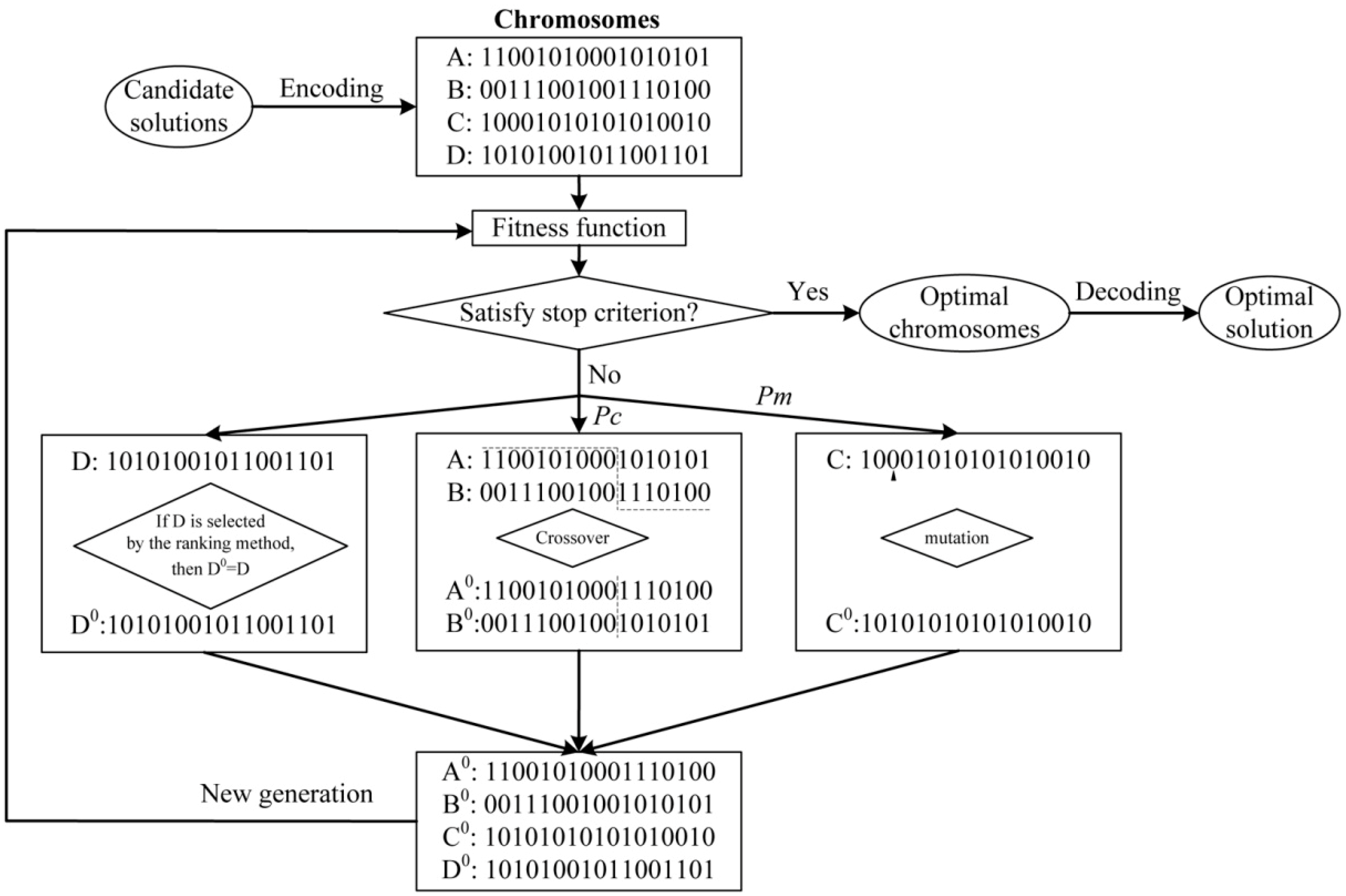
3.2. Optimisation through Self-Adaptive Genetic Algorithm
3.2.1. Encoding the Chromosomes
3.2.2. The Fitness Function

3.2.3. Selection, Crossover and Mutation

3.3. Model Implementation
4. Results
4.1. The Optimal Chromosome/CA Transition Rules

| Variables | Parameters | |
|---|---|---|
| Logistic | SAGA | |
| a0 (Constant) | −0.77 | −0.82 |
| a1 (I_external) | 1.02 | 1.19 |
| a2 (d_centres) | −0.98 | −1.13 |
| a3 (d_agri) | 0.93 | 0.98 |
| a4 (d_road) | −1.09 | −1.05 |
| a5 (d_rail) | 0.41 | 0.58 |
| a6 (d_railstn) | −1.15 | −1.11 |
| a7 (d_rivers) | 0.75 | 0.68 |
| a8 (SLOPE) | −0.34 | −0.34 |
| a9 (DEM) | −0.91 | −1.12 |
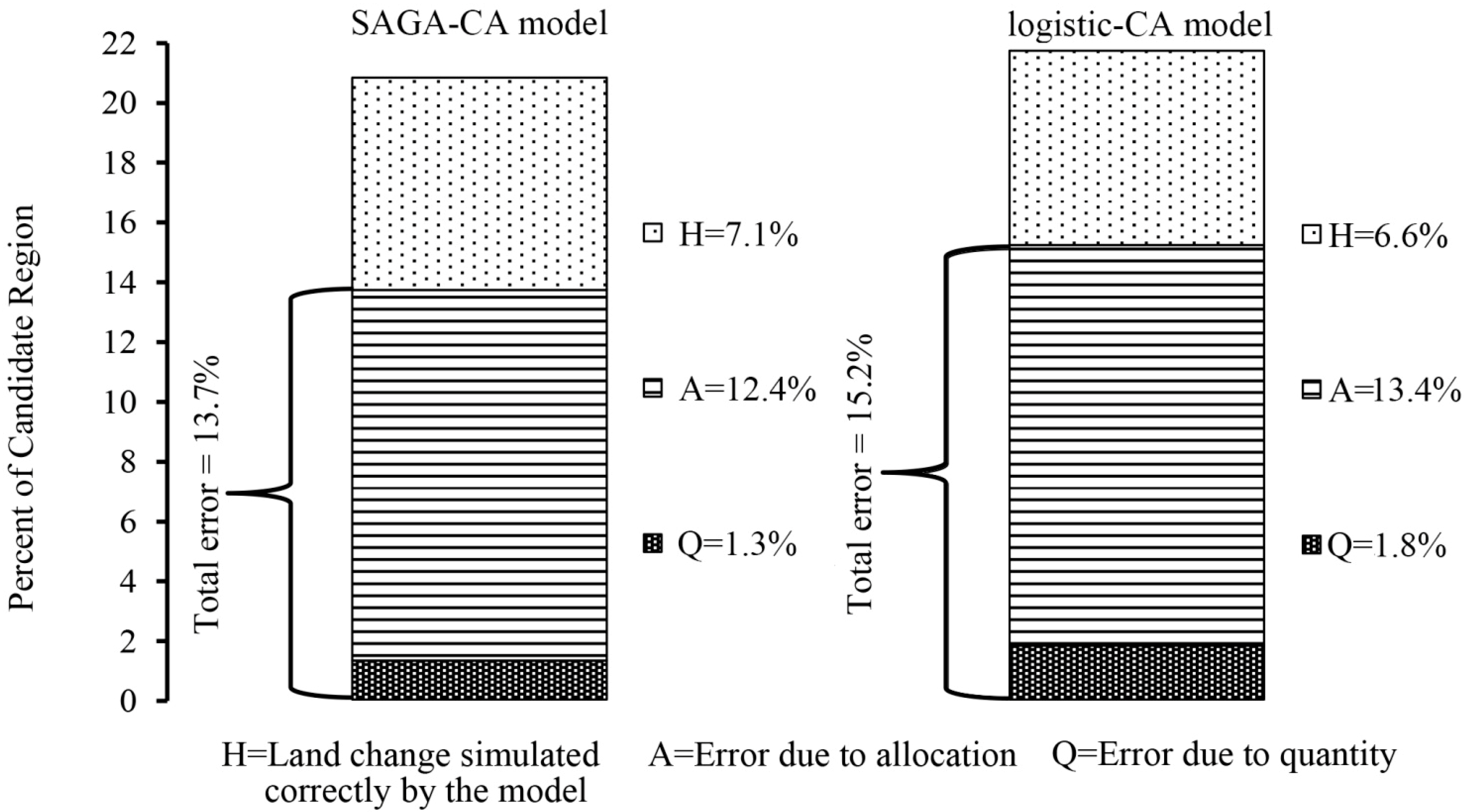
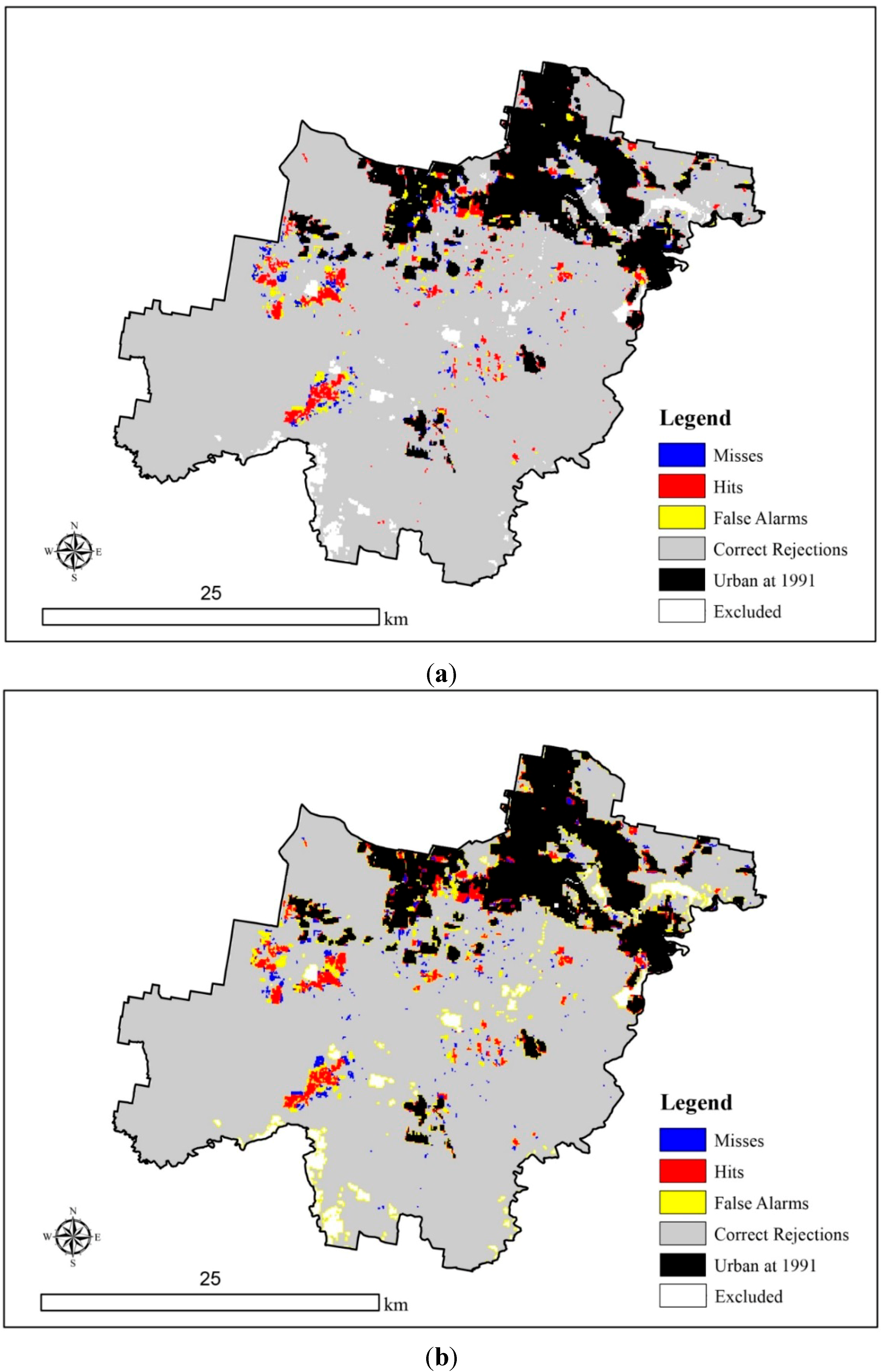
4.2. Simulation Accuracies of the SAGA-CA Model


5. Discussion
6. Conclusions
Author Contributions
Conflicts of Interest
References
- White, R.W.; Engelen, G. Cellular automata and fractal urban form: A cellular modelling approach to the evolution of urban land use patterns. Environ. Plan. A Environ. Plan. 1993, 25, 1175–1193. [Google Scholar]
- Clarke, K.C.; Gaydos, L. Loose-coupling a cellular automaton model and GIS: Long-term urban growth prediction for San Francisco and Washington/Baltimore. Int. J. Geogr. Inf. Sci. 1998, 12, 699–714. [Google Scholar] [CrossRef]
- Wu, F. SimLand: A prototype to simulate land conversion through the integrated GIS and CA with AHP-derived transition rules. Int. J. Geogr. Inf. Sci. 1998, 12, 63–82. [Google Scholar] [CrossRef]
- Batty, M.; Xie, Y.; Sun, Z. Modelling urban dynamics through GIS-based cellular automata. Comput. Environ. Urban Syst. 1999, 23, 205–233. [Google Scholar] [CrossRef]
- Wu, F. Calibration of stochastic cellular automata: The application to rural-urban land conversions. Int. J. Geogr. Inf. Sci. 2002, 16, 795–818. [Google Scholar] [CrossRef]
- Liu, Y.; Phinn, S.R. Modelling urban development with cellular automata incorporating fuzzy-set approaches. Comput. Environ. Urban Syst. 2003, 27, 637–658. [Google Scholar] [CrossRef]
- He, C.Y.; Okada, N.; Zhang, Q.F.; Shi, P.J.; Zhang, J.S. Modelling urban expansion scenarios by coupling cellular automata model and system dynamic model in Beijing, China. Appl. Geogr. 2006, 26, 323–345. [Google Scholar] [CrossRef]
- Stevens, D.; Dragićević, S. A GIS-based irregular cellular automata model of land-use change. Environ. Plan. B Plan. Des. 2007, 34, 708–724. [Google Scholar] [CrossRef]
- Stevens, D.; Dragićević, S.; Rothley, K. iCity: A GIS-CA modelling tool for urban planning and decision making. Environ. Model. Softw. 2007, 22, 761–773. [Google Scholar] [CrossRef]
- Dietzel, C.; Clarke, K.C. Toward optimal calibration of the SLEUTH land use change model. Trans. GIS 2007, 11, 29–45. [Google Scholar]
- Al-kheder, S.; Wang, J.; Shan, J. Fuzzy inference guided cellular automata urban-growth modelling using multi-temporal satellite images. Int. J. Geogr. Inf. Sci. 2008, 22, 1271–1293. [Google Scholar] [CrossRef]
- Al-Ahmadi, K.; See, L.; Heppenstall, A.; Hogg, J. Calibration of a fuzzy cellular automata model of urban dynamics in Saudi Arabia. Ecol. Complex. 2009, 6, 80–101. [Google Scholar] [CrossRef]
- Mondal, P.; Southworth, J. Evaluation of conservation interventions using a cellular automata-Markov model. For. Ecol. Manag. 2010, 260, 1716–1725. [Google Scholar] [CrossRef]
- Heppenstall, A.; See, L.; Al-Ahmadi, K.; Kim, B. CA City: Simulating urban growth through the application of Cellular Automata. In Cellular Automata—Simplicity behind Complexity; Salcido, A., Ed.; InTech: Winchester, UK, 2011; pp. 87–104. [Google Scholar]
- Feng, Y.; Liu, Y.; Tong, X.; Liu, M.; Deng, S. Modeling dynamic urban growth using cellular automata and particle swarm optimization rules. Landsc. Urban Plan. 2011, 102, 188–196. [Google Scholar] [CrossRef]
- Liu, Y. Modelling sustainable urban growth in a rapidly urbanising region using a fuzzy-constrained cellular automata approach. Int. J. Geogr. Inf. Sci. 2012, 26, 151–167. [Google Scholar] [CrossRef]
- Vaz, E.; Nijkamp, P.; Painho, M.; Caetano, M. A multi-scenario forecast of urban change: Astudy on urban growth in the Algarve. Landsc. Urban Plan. 2012, 104, 201–211. [Google Scholar] [CrossRef]
- Chaudhuri, G.; Clarke, K.C. The SLEUTH land use change model: A review. Int. J. Environ. Resour. Res. 2013, 1, 88–104. [Google Scholar]
- Santé, I.; García, A.M.; Miranda, D.; Crecente, R. Cellular automata models for the simulation of real-world urban processes: A review and analysis. Landsc. Urban Plan. 2010, 96, 108–122. [Google Scholar] [CrossRef]
- Ward, D.P.; Murray, A.T.; Phinn, S.R. A stochastically constrained cellular model of urban growth. Comput. Environ. Urban Syst. 2000, 24, 539–558. [Google Scholar] [CrossRef]
- White, R.; Engelen, G.; Uljee, I. The use of constrained cellular automata for high-resolution modelling of urban land-use dynamics. Environ. Plan. B Plan. Des. 1997, 24, 323–343. [Google Scholar]
- Almeida, C.M.; Gleriani, J.M.; Castejon, E.F.; Soares-Filho, B.S. Using neural networks andcellular automata for modelling intra-urban land-use dynamics. Int. J. Geogr. Inf. Sci. 2008, 22, 943–963. [Google Scholar] [CrossRef]
- Wu, F. Simulating urban encroachment on rural land with fuzzy-logic-controlled cellular automata in a geographical information system. J. Environ. Manag. 1998, 53, 293–308. [Google Scholar] [CrossRef]
- Li, L.; Sato, Y.; Zhu, H. Simulating spatial urban expansion based on a physical process. Landsc. Urban Plan. 2003, 64, 67–76. [Google Scholar] [CrossRef]
- Feng, Y.; Liu, Y. A heuristic cellular automata approach for modelling urban land-use change based on simulated annealing. Int. J. Geogr. Inf. Sci. 2013, 27, 449–466. [Google Scholar] [CrossRef]
- Feng, Y.; Liu, Y. A cellular automata model based on nonlinear kernel principal component analysis for urban growth simulation. Environ. Plan. B 2013, 40, 116–134. [Google Scholar] [CrossRef]
- Tayyebi, A.; Delavar, M.R.; Pijanowski, B.C.; Yazdanpanah, M.J.; Saeedi, S.; Tayyebi, A.H. A spatial logistic regression model for simulating land use patterns, a case study of the Shiraz metropolitan area of Iran. In Advances in Earth Observation of Global Change; Chuvieco, E., Li, J., Yang, X., Eds.; Springer: Berlin, Germany, 2010; pp. 27–42. [Google Scholar]
- Wu, F.; Webster, C.J. Simulation of land development through the integration of cellular automata and multi-criteria evaluation. Environ. Plan. B Plan. Des. 1998, 25, 103–126. [Google Scholar]
- Arsanjani, J.J.; Helbich, M.; Kainz, W.; Boloorani, A.D. Integration of logistic regression, Markov chain and cellular automata models to simulate urban expansion. Int. J. Appl. Earth Obs. Geoinf. 2013, 21, 265–275. [Google Scholar] [CrossRef]
- Glen, W.G.; Dunn, W.J.; Scott, D.R. Principal components analysis and partial least squares regression. Tetrahedron Comput. Methodol. 1989, 2, 349–376. [Google Scholar] [CrossRef]
- Bies, R.R.; Muldoon, M.F.; Pollock, B.G.; Manuck, S.; Smith, G.; Sale, M.E. A genetic algorithm-based, hybrid machine learning approach to model selection. J. Pharmacokinet. Pharmacodyn. 2006, 33, 196–221. [Google Scholar]
- Xu, X.; Zhang, J.; Zhou, X. Integrating GIS, cellular automata, and genetic algorithm in urban spatial optimization: A case study of Lanzhou. Proc. SPIE 2006, 6420. [Google Scholar] [CrossRef]
- Li, X.; Yang, Q.S.; Liu, X.P. Genetic algorithms for determining the parameters of cellular automata in urban simulation. Sci. China Ser. D Earth Sci. 2007, 50, 1857–1866. [Google Scholar] [CrossRef]
- Clarke-Lauer, M.D.; Clarke, K.C. Evolving simulation modeling: Calibrating SLEUTH using a genetic algorithm. In Proceedings of the 11th International Conference on GeoComputation, London, UK, 20–22 July 2011.
- Feng, Y.; Liu, Y.; Han, Z. Land use simulation and landscape assessment using genetic algorithm based cellular automata under different sampling schemes. Chin. J. Appl. Ecol. 2011, 22, 957–963. [Google Scholar]
- Feng, Y.; Liu, Y. An optimized cellular automata based on adaptive genetic algorithm for urban growth simulation. In Advances in Spatial Data Handling and GIS:Lecture Notes in Geoinformatics and Cartography; Yeh, A.G.O., Shi, W., Leung, Y., Zhou, C., Eds.; Springer-Verlag: Berlin/Heidelberg, Germany, 2012; Part 2; pp. 27–38. [Google Scholar]
- Schmitt, L.M.; Nehaniv, C.L.; Fujii, R.H. Linear analysis of genetic algorithms. Theor. Comput. Sci. 1998, 208, 111–148. [Google Scholar] [CrossRef]
- Jenerette, G.D.; Wu, J. Analysis and simulation of land-use change in the central Arizona—Phoenix region, USA. Landsc. Ecol. 2001, 16, 611–626. [Google Scholar] [CrossRef]
- Stewart, T.J.; Janssen, R.; Herwijnen, M.V. A genetic algorithm approach to multi-objective land use planning. Comput. Oper. Res. 2004, 31, 2293–2313. [Google Scholar] [CrossRef]
- Matthews, K.B.; Buchan, K.; Sibbald, A.R.; Craw, S. Combining deliberative and computer-based methods for multi-objective land-use planning. Agric. Syst. 2006, 87, 18–37. [Google Scholar] [CrossRef]
- Cao, K.; Batty, M.; Huang, B.; Liu, Y.; Yu, L.; Chen, J.F. Spatial multi-objective land use optimization: Extensions to the non-dominated sorting genetic algorithm-II. Int. J. Geogr. Inf. Sci. 2011, 25, 1949–1969. [Google Scholar] [CrossRef]
- Shan, J.; Alkheder, S.; Wang, J. Genetic algorithms for the calibration of cellular automata urban growth modeling. Photogramm. Eng. Remote Sens. 2008, 74, 1267–1277. [Google Scholar] [CrossRef]
- Seppelt, R.; Voinov, A. Optimization methodology for land use patterns using spatially explicit landscape models. Ecol. Model. 2002, 151, 125–142. [Google Scholar] [CrossRef]
- Mitchell, M.; Crutcheld, J.P.; Das, R. Evolving cellular automata with genetic algorithms: A review of recent work. In Proceedings of the First International Conference on Evolutionary Computation and Its Applications (EvCA’96), Moscow, Russia, 1–4 June 1996.
- Tang, J.; Wang, L.; Yao, Z. Spatio-temporal urban landscape change analysis using the Markov chain model and a modified genetic algorithm. Int. J. Remote Sens. 2007, 28, 3255–3271. [Google Scholar] [CrossRef]
- Li, X.; Lin, J.; Chen, Y.; Liu, X.; Ai, B. Calibrating cellular automata based on landscape metrics by using genetic algorithms. Int. J. Geogr. Inf. Sci. 2013, 27, 594–613. [Google Scholar] [CrossRef]
- García, A.M.; Santé, I.; Boullón, M.; Crecente, R. Calibration of an urban cellular automaton model by using statistical techniques and a genetic algorithm. Application to a small urban settlement of NW Spain. Int. J. Geogr. Inf. Sci. 2013, 27, 1593–1611. [Google Scholar] [CrossRef]
- Queensland Local Government Reform Commission. Report of the Local Government Reform Commission; Queensland Government: Brisbane, QLD, Australia, 2007; Volume 2. [Google Scholar]
- Australian Bureau of Statistics. Census Product 2011. Available online: http://www.abs.gov.au/ (accessed on 1 October 2013).
- Queensland Government. Statewide Landcover and Trees Study (SLATS). Available online: http://www.qld.gov.au/environment/land/vegetation/mapping/slats/ (accessed on 30 June 2014).
- Danaher, T.; Scarth, P.; Armston, J.; Collett, L.; Kitchen, J.; Gillingham, S. Remote sensing of tree-grass systems: The Eastern Australian woodlands. In Ecosystem Function in Savannas: Measurement and Modeling at Landscape to Global Scales; Hill, M.J., Hanan, N.P., Eds.; CRC Press: Boca Raton, FL, USA, 2010; pp. 175–194. [Google Scholar]
- Collett, L.; Goulevitch, B.M.; Danaher, T.J. SLATS radiometric correction: A semi-automated multi stage process for the standardisation of temporal and spatial radiometric differences. In Proceedings of the 9th Australasian Remote Sensing and Photogrammetry Conference, Sydney, NSW, Australia, 24 July 1998.
- Australian Bureau of Statistics. Census Product 2006. Available online: http://www.abs.gov.au/ (accessed on 1 October 2013).
- Liu, Y.; Feng, Y.J. A logistic based cellular automata model for continuous urban growth simulation: A case study of the Gold Coast City, Australia. In Agent-Based Models of Geographical Systems; Heppenstall, A.J., Crooks, A.Y., See, L.M., Batty, M., Eds.; Springer: Dordrecht, The Netherlands, 2012; pp. 643–662. [Google Scholar]
- Muzy, A.; Nutaro, J.J.; Zeigler, B.P.; Coquillard, P. Modelling landscape dynamics in an Atlantic rainforest region: Implications for conservation. Ecol. Model. 2008, 219, 212–225. [Google Scholar] [CrossRef]
- Goldberg, D.E.; Holland, J.H. Genetic algorithms and machine learning. Mach. Learn. 1988, 3, 95–99. [Google Scholar] [CrossRef]
- Mardle, S.; Pascoe, S. An overview of genetic algorithms for the solution of optimisation problems. Comput. High. Educ. Econ. Rev. 1999, 13, 16–20. [Google Scholar]
- Angeline, P.J. Adaptive and self-adaptive evolutionary computation. In Computational Intelligence: A Dynamic System Perspective; IEEE Press: New York, NY, USA, 1995; pp. 152–161. [Google Scholar]
- Srinivas, M.; Patnaik, L.M. Adaptive probabilities of crossover and mutation in genetic algorithms. IEEE Trans. Syst. Man Cybern. 1994, 24, 656–667. [Google Scholar] [CrossRef]
- Houck, C.R.; Joines, J.A.; Kay, M.G. A Genetic Algorithm for Function Optimization: A Matlab Implementation; Technical Report NCSU-IE-TR-95–09; North Carolina State University: Raleigh, NC, USA, 1995; pp. 1–14. [Google Scholar]
- Pontius, R.G.; Peethambaram, S.; Castella, J. Comparison of three maps at multiple resolutions: A case study of land change simulation in Cho Don District, Vietnam. Ann. Assoc. Am. Geogr. 2011, 101, 45–62. [Google Scholar] [CrossRef]
- Pontius, R.G.; Shusas, E.; McEachern, M. Detecting important categorical land changes while accounting for persistence. Agric. Ecosyst. Environ. 2004, 101, 251–268. [Google Scholar] [CrossRef]
- Pontius, R.G.; Malanson, J. Comparison of the structure and accuracy of two land change models. Int. J. Geogr. Inf. Sci. 2005, 19, 243–265. [Google Scholar] [CrossRef]
- Pontius, R.G.; Millones, M. Death to Kappa: Birth of quantity disagreement and allocation disagreement for accuracy assessment. Int. J. Remote Sens. 2011, 32, 4407–4429. [Google Scholar] [CrossRef]
- Chen, H.; Pontius, R.G. Diagnostic tools to evaluate a spatial land change projection along a gradient of an explanatory variable. Landsc. Ecol. 2010, 25, 1319–1331. [Google Scholar] [CrossRef]
- Kocabas, V.; Dragićević, S. Assessing cellular automata model behaviour using a sensitivity analysis approach. Comput. Environ. Urban Syst. 2006, 30, 921–953. [Google Scholar] [CrossRef]
© 2014 by the authors; licensee MDPI, Basel, Switzerland. This article is an open access article distributed under the terms and conditions of the Creative Commons Attribution license (http://creativecommons.org/licenses/by/3.0/).
Share and Cite
Liu, Y.; Feng, Y.; Pontius, R.G., Jr. Spatially-Explicit Simulation of Urban Growth through Self-Adaptive Genetic Algorithm and Cellular Automata Modelling. Land 2014, 3, 719-738. https://doi.org/10.3390/land3030719
Liu Y, Feng Y, Pontius RG Jr. Spatially-Explicit Simulation of Urban Growth through Self-Adaptive Genetic Algorithm and Cellular Automata Modelling. Land. 2014; 3(3):719-738. https://doi.org/10.3390/land3030719
Chicago/Turabian StyleLiu, Yan, Yongjiu Feng, and Robert Gilmore Pontius, Jr. 2014. "Spatially-Explicit Simulation of Urban Growth through Self-Adaptive Genetic Algorithm and Cellular Automata Modelling" Land 3, no. 3: 719-738. https://doi.org/10.3390/land3030719
APA StyleLiu, Y., Feng, Y., & Pontius, R. G., Jr. (2014). Spatially-Explicit Simulation of Urban Growth through Self-Adaptive Genetic Algorithm and Cellular Automata Modelling. Land, 3(3), 719-738. https://doi.org/10.3390/land3030719